Hydrodynamic Analysis of Horizontal Axis Tidal Current Turbine under the Wave-Current Condition

Abstract

To take advantage of the high tidal current velocity near the free surface, the horizontal axis turbine is installed, which inevitably causes hydrodynamic characteristics to effect the turbine by the waves. In this article, we established a numerical calculation method for the hydrodynamic load of a horizontal axis turbine under wave-current conditions. Based on the numerical calculation results, the hydrodynamic loads were decomposed and the influence rules of wave parameters and blade tip immersion depth on the hydrodynamic load were obtained. The study found the following: (1) the multi-frequency fluctuations based on the rotation frequency and incident wave frequency occurred in instantaneous values of the axial load coefficients and energy utilization ratios, and the fluctuation amplitude decreased with the increase of the blade tip immersion depth; (2) the fluctuation amplitude, according to rotation frequency, changed less with the increase of wave period and wave height, and was smaller according to wave frequency; (3) the fluctuation amplitude based on wave frequency increased linearly with the increase of wave height and wave period. The research results can provide the basis and reference for the design and engineering application of tidal current power station.

1. Introduction

Tidal current power can be described as a highly dense, reliable, and predictable renewable energy source. It has been reported that an available tidal power of 95 and 61.3 TWH/year are available in the UK and China, respectively [1,2]. To make full use of the high flow velocity of the water’s surface in actual horizontal axis tide power stations, horizontal axis turbine is generally supported by floating type or fixed carriers from the bottom of the sea toward near the free surface [3]. The turbine faces the effects of water cavitation, free surface, and velocity gradient caused by waves. The impact not only makes turbine power characteristics worse but also causes accumulation of interference load, fatigue, and turbine fracture or support structure, which can lead to major accidents.

When the horizontal axis tidal current energy turbine runs near the free-surface, the movement of the turbine causes the deformation of the wave surface and vice versa [4,5,6,7,8]. The interacting of the turbine and the wave involves the unsteady and nonlinear interaction between the vortex, turbulence, and wave surface, which complicates the flow field around the turbine. Therefore, it is important to accurately predict the hydrodynamic performance of a horizontal axis turbine under wave conditions. Recently, great interest has developed for turbine dynamic loading as a result of wave-current interactions. Many experimental and numerical studies have investigated the dynamic behavior of scale model horizontal axis tidal current turbine performance immersed in towing and flume tanks, which highlights the strong influence of surface waves [9,10,11,12,13,14,15,16]. It was reported that the mean values of both power and thrust coefficients in the presence of waves were identical to cases of current conditions.

In 2007, Barltrop et al. [9] studied the influence of waves on the tidal current turbines. In the towing pool, the 3-blade horizontal axis turbine was tested. The turbine radius was 0.16 m, airfoil S814, and maximum chord length was 66.5 mm. The average value of torque and thrust within a range of the turbine’s regular wave and Reynolds number range were measured, where the relative velocity on the turbine radius of 0.7 was tested. The results show that there was no difference between each parameter’s average value and the wave-free condition, yet the instantaneous value of thrust and torque obviously changed. In 2010, Gallway et al. [10] also carried out similar model tests on the three-blade horizontal axis turbine in the towing basin. The turbine diameter was 0.5 m and the regular deep-water wave (wavelength/depth) was 0.4 m. These results are similar to Barltrop’s, who found that the instantaneous change of thrust is about 37% and torque 35%. In 2013, Benoit et al. [11] tested a three-blade horizontal axis turbine with a diameter of 0.8 m in an experimental towing basin. The test results show that interaction between wave and current increases the load fluctuation amplitude, which must be considered in fatigue analysis. In 2014, Henriques et al. [12] carried out a surface wave model test on a three-blade horizontal axis turbine in a high-speed circulating tank at the University of Liverpool, measuring the thrust and power of the turbine under two different regular wave conditions and comparing the measurement results with those under uniform flow (no wave) conditions. A similar conclusion was obtained: the average value of thrust and power coefficient of the turbine under regular wave condition was basically the same as the measured value of uniform flow, yet the instantaneous value had obvious periodic change, and the change frequency was consistent with the wave frequency. In recent years, similar hydrodynamic tests of wave turbines were carried out by Ethan [13], Pascal [14], and Mustafa [15]. In 2019, Zhang Jisheng [16] carried out a physical model test to explore the velocity change and turbulent characteristics of the wake field of a horizontal axis tidal current turbine under the interaction of waves and flows. Compared with the condition without waves, the existence of waves was conducive to the recovery of the water flow behind the supporting structure, yet it caused a bigger loss of near wake velocity behind the water area where the turbine blades rotated. The turbulence intensity decreased when the wave period increased and increased when the wave height increased. In 2013, Harbin Engineering University (HEU) successfully developed and installed the "Haineng II" 200 kW floating horizontal axis tidal current power station, whose operation on the sea shows that waves have a significant impact on turbine power characteristics and floating carrier motion.

Most previous numerical studies that used the blade-element momentum (BEM) model to evaluate the dynamic loading behavior of the horizontal axis tidal current turbine due to surface wave’s effects utilized linear wave theory to estimate the horizontal and vertical wave particle velocities [14,17,18]. The main problem of linear wave theory is that the current effects on waves are not accounted for; the current velocity is simply superimposed to the horizontal wave particle velocities. On the other hand, the BEM model based on the lift and drag obtained from two-dimensional airfoil cannot be used to analyze complex three-dimensional flow effects, nor can it obtain detailed flow field information.

It can be seen from the above research that the hydrodynamic problem of horizontal axis turbine under wave-flow condition was mainly studied by a model test. Then, the variation trend of the hydrodynamic load of the turbine under wave-flow condition was obtained, but the specific rules about the influence of wave parameters on the load are not given. Therefore, in this article, based on the computational fluid dynamics (CFD) method, the hydrodynamic load was calculated within the horizontal axis turbine under wave-current conditions. The hydrodynamic loads decomposed, and the influence rules of wave parameters and the blade tip immersion depth on those loads were obtained. Further, we summarized the approximate fast prediction method about hydrodynamic load under wave-current condition. Lastly, we provided, the reference of hydrodynamic load forecast for the horizontal axis of the turbine under complex condition.

2. CFD Numerical Simulations

2.1. Calculation Model

CFD simulations were performed with the node centered in a finite volume solver. The fluid region was meshed to be decomposed into a finite number of a controlled volume. For incompressible fluids, the general conservation (transport) equation for continuity and momentum given below were solved on the set of controlled volume:

$$\frac{\partial u_i}{\partial x_i}=0$$

(1)

$$\rho \frac{\partial u_i}{\partial t}+\rho u_j\frac{\partial u_i}{\partial x_j}=f_i-\frac{\partial p_i}{\partial x_i}+\mu {\nabla }^2{u}_i$$

(2)

The blades used in the turbine calculation model were developed by the Institute of Renewable Energy, Deep Sea Center, and Harbin Engineering University [19]. We adopted a cross-sectional airfoil with a S809 blade extending, as well as the form of varying chord length and pitch angle. The chord length and pitch angle of different radius sections are shown in

Table 1. Parameters of the turbine.

Radius (mm)	Chord (mm)	Pitch (Degrees)
70	90.01	26.2
90	84.96	19.9
110	80.11	15.5
130	75.46	12.2
150	71.01	9.8
170	66.76	7.9
190	62.71	6.3
210	58.86	5.0
230	55.21	4.0
250	51.76	3.1
270	48.51	2.3
290	45.46	1.6
310	42.61	1.1
330	39.96	0.5
350	37.51	0.1

and Figure 1. The turbine diameter in the model was 0.7 m and there were two blades (Figure 2a). After the calculation model was built, a large enough calculation field was given to simulate the flow field. The distances of the turbine rotation plane from the inlet and outlet boundaries of the calculation field were 5D and 15D, respectively. Moreover, the distance from the bottom and the side to the turbine rotating shaft were 5D. Since the simulation was a two-phase flow, the distance between the turbine rotating shaft and the top side of the calculation field was 2D to reduce the calculation time. To avoid a reduction in grid quality during the calculation process, the entire computational domain was divided into two parts: rotation domain and static domain. For convenience, a fixed coordinate system was established. The origin of the coordinate system was located on the turbine axis. The XOZ plane was parallel to the stationary water surface. The z-axis was in the direction of tidal current and the Y-axis was in the vertical direction.

2.2. Mesh Generation

In this paper, a hexahedron-based mesh form was adopted. A previous work [20] studied the number and convergence of meshes. The results showed that when the number of meshes reaches 2.31 million and the height of the first layer of mesh on the model surface was 0.0005 m, the calculation results were basically unchanged even if the mesh was encrypted. In this paper, the mesh was refined based on a previous method [20], which improved the blade surface’s mesh quality and encrypted the region of the wave height range. The height of the turbine surface mesh of the first layer height was 0.0005 m, the stretching ratio was 1.1, and the y+ ranges was 0.7-48, as shown in Figure 2b. The target size and minimum size of turbine surface were 0.002 m and 0.0005 m, respectively, as shown in Figure 2c. Specifically, 12 grids were divided in the wave height range and 100 girds were divided in the wavelength range. Since the turbine formed a wave-maker, the mesh in the free surface area near the turbine was further encrypted, as shown in Figure 2d.

2.3. Boundary Condition Setting

For the CFD system, the Unsteady Reynold Averaged Navier Stokes (URANS) equations were solved with a transient rotor-stator approach. A sliding mesh technique was utilized to physically rotate the rotation domain. The shear stress transport (SST) turbulence model was used with an automatic wall function approach. The SST turbulence model can accurately predict the onset and amount of flow separation in adverse pressure gradients. The SST model demonstrated better flow separation prediction and more accurate performance assessment in several turbine CFD studies [21,22]. The wall function model utilized the log law approximation and provided better computational efficiency.

The numerical simulation was completed by the CFD Software and based on the volume of fluid (VOF) method to simulate two-phase flow. The VOF regular wave model was established first and then the static water surface position, water velocity, air velocity, wave period, and amplitude were given. The other relevant settings are as follows: the atmospheric pressure was set as the standard pressure and then the direction of gravitational acceleration was obtained; the inlet boundary was set as the velocity inlet condition and then the velocity of VOF regular wave model and the volume fraction of water and air were given; the outlet boundary was set as an open pressure boundary, the relative pressure and the volume fraction of water and air were then given; the left and right sides of the fluid computing domain were set as free slip wall surfaces; the top and the bottom of the fluid calculation domain was set as a velocity inlet condition and the velocity of VOF regular wave model and the volume fraction of water and air were given; the surface of blade and hub was set as a non-slip wall; a sliding mesh technique was utilized to physically rotate the rotation domain and then the rotation angular velocity in the rotation domain was given; the static domain and the rotational domain were connected by an interface; a transient solver was used. The boundary conditions were then set, as shown in Figure 3. In addition, the turbulence model used in this study was the SST k-omega turbulence model, which Menter proposed in 1994 [23]. It can accurately predict the onset and amount of flow separation in adverse pressure gradients and demonstrated better flow separation prediction and more accurate performance assessment in several turbine CFD studies [21,22,24]. The time stepping [25] was set as the rotation time of the blades rotate 3° around the Z-axis. In the computing process, spatial discrete used high-resolution scheme, which owns second-order or higher order accuracy. Moreover, temporal discrete adopted a second-order implicit scheme.

3. Result and Analysis

3.1. Validation of Uniform Flow

The above grid model and boundary condition set were used to simulate the test conducted by the Institute of Renewable Energy and HEU research (Inflow velocity U = 1.5 m/s, tip-immersion H = 0.79D) [26]. Then, the energy utilization ratio and axial load coefficient of the turbine with different rotation speed were obtained. Energy utilization ratio ($C_P$) of the turbine was a parameter that represented the ability of a turbine to absorb tidal current kinetic energy. The axial load coefficient ($C_Z$) of the turbine was the dimensionless load along the rotation axis and the blade tip speed ratio ($\lambda$) was the ratio of blade tip rotational linear velocity to incoming flow velocity. These can be expressed as:

$$C_P=\frac{T_Z\omega }{\frac{1}{2}\rho U^3\pi R^2}$$

(3)

$$C_Z=\frac{F_Z}{\frac{1}{2}\rho U^2\pi R^2}$$

(4)

$$\lambda =\frac{{\omega }_{T}R}{U}$$

(5)

The comparison between the experimental values and the average values of the calculated results are shown in Figure 4. The average value refers to the arithmetic average of the calculated results when the turbine rotates once. It can be seen that the calculated value and the experimental value were basically the same. The result verified the feasibility and accuracy of the numerical method on studying the hydrodynamic characteristics of the horizontal axis turbine under two-phase flow conditions. It should be noted that, since HEU measures the output power of the generator during the turbine test, the experimental data in the figure was the measured data divided by 0.85 (consider generator conversion efficiency and mechanical transmission efficiency).

3.2. Wave Simulation Validity Verification

When there was no turbine, the mesh model and boundary condition settings in Section 1 were used to simulate the coupling of regular waves (wave height 0.09 m, period 1.3 s) and uniform incoming flow (1.5 m/s). As shown in Figure 5, the change of the Z coordinate on the free surface and 5D away from the inlet boundary was monitored and compared with the theoretical values based on Stokes’ first-order wave theory.

In Figure 5, it can be seen that the CFD numerical results changed slightly, but basically coincided with the theoretical values, verifying the effectiveness of the numerical method on wave simulation used in this paper. It should be noted that the given wave period 1.3 was the relative period when the wave and current were coupled, while the actual surface fluctuations change according to the regular wave period when there was no flow velocity, and the relationship is as follows:

$${\omega }_w={\omega }_r+k_{r}U$$

(6)

3.3. Influence of the Blade Tip Immersion Depth on Hydrodynamic Performance of the Turbine

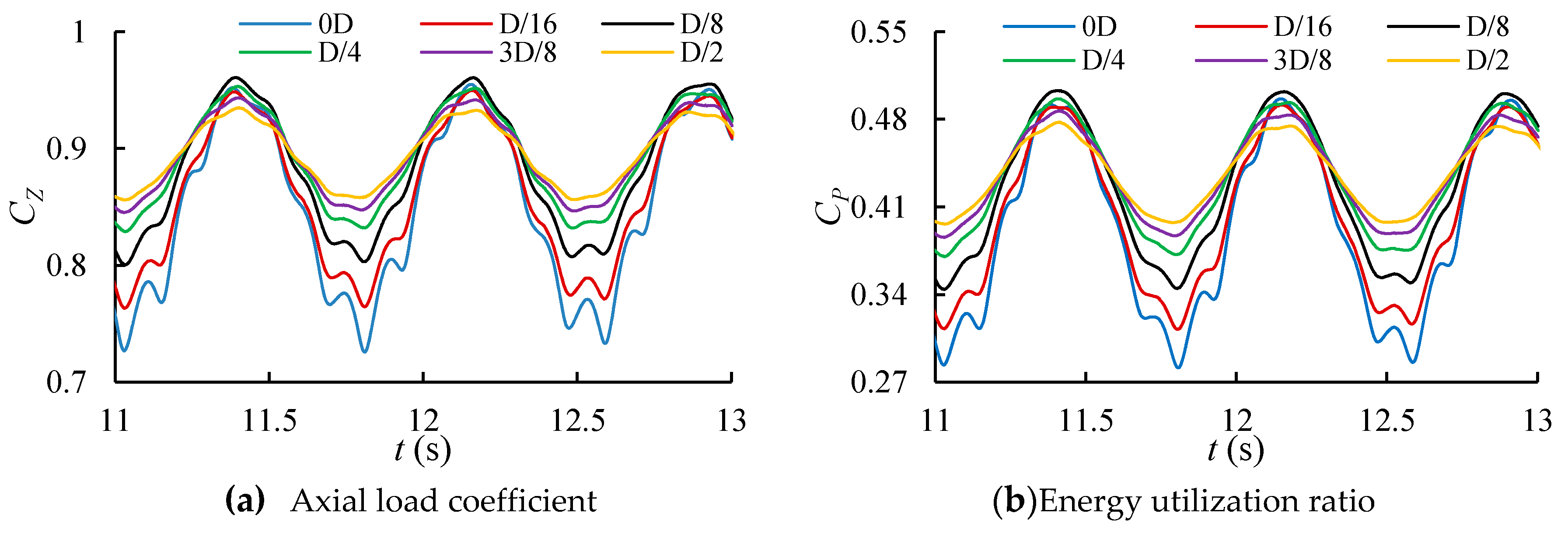
The wave height was set at 0.09 m, the relative wave period was 1.3 s, and the rotation speed was 230 r/min. The hydrodynamic load of the different blade tip immersion depth under water was calculated. The time-history curves of axial load coefficient and energy utilization ratio of the blade wheel under different blade tip immersion water depth were obtained and compared with those under free surface condition only, as shown in Figure 6.

As seen in the figure, the existence of the wave caused the turbine axis load and energy utilization to fluctuate. The overall fluctuation frequency was equal to the corresponding wave frequency when there was no flow velocity. With the increase of blade tip immersion depth, the fluctuation amplitude of axial load coefficient and energy utilization ratio decreased gradually, and the average value increased.

3.4. Influence of Wave Period on Hydrodynamic Performance of the Turbine

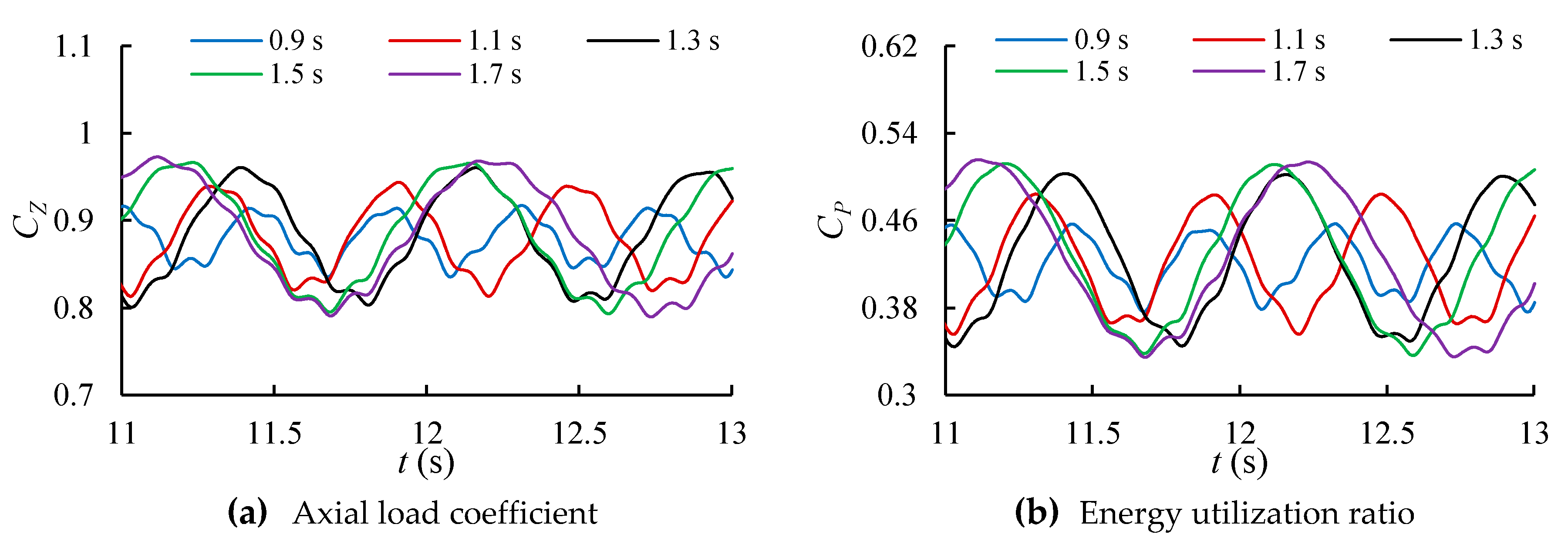
In this paper, the blade tip immersion depth D/8, wave amplitude was 0.09 m and the speed was 230 r/min. Five relative wave periods (0.9 s, 1.1 s, 1.3 s, 1.5 s, and 1.7 s) were selected for the following numerical simulation. The time-history curves of axial load coefficients and energy utilization ratios of the turbine under different wave periods were obtained, as shown in Figure 7.

It can be seen that with the increase of wave period, the fluctuation amplitudes of the axial load coefficients and turbine’s energy utilization ratios gradually increased because the wave propagation speed increased with the increase of the wave period. We also found that the time-mean values of the axial load coefficients and energy utilization ratios changed only a little.

3.5. Influence of Wave Height on Hydrodynamic Performance of the Turbine

The blade tip immersion depth under water was set as D/8, the relative wave period was 1.3 s, and the rotation speed was 230 r/min. Five wave heights (0.05 m, 0.07 m, 0.09 m, 0.11 m, and 0.13 m) were selected for numerical simulation. The time-history curves of the axial load coefficient and energy utilization ratio of the turbine under different wave amplitudes were obtained, as shown in Figure 8.

As seen in the above figure, with the increase of wave height, the fluctuation amplitudes of axial load coefficients and energy utilization ratios gradually increased, but the fluctuation period and the time-mean value of the axial load coefficients and energy utilization ratios were basically the same. This was because the wave frequency was the same and the motion velocity of the fluid particle increased with the increase of wave height.

4. Load Decomposition Analysis

According to the time-history curve under the wave condition, the axial load coefficients and energy utilization ratios fluctuated in multiple frequencies based on the rotation frequency of the turbine and the wave frequency when the flow velocities were zero. Therefore, the axial load coefficient and energy utilization can be written as the following series:

$$\begin{array}{ll}{C}_Z& =C_Z^0+{\displaystyle \sum _{i_0=1}^{m_0}{C}_Z^{i_0}\sin \left(i_{0}N{\omega }_T+{\psi }_{ZT}^{i_0}\right)}\\ & +{\displaystyle \sum _{j=1}^{n_1}\left(C_{Z1}^{0j}+{\displaystyle \sum _{i_1=1}^{m_1}{C}_{Z1}^{ij}\sin \left(i_{1}N{\omega }_T+{\psi }_{ZT1}^{i_1}\right)}\right)\sin \left(j{\omega }_W\right)}\\ & +{\displaystyle \sum _{k=1}^{n_2}\left(C_{Z2}^{0k}+{\displaystyle \sum _{i_2=1}^{m_2}{C}_{Z2}^{ik}\sin \left(i_{2}N{\omega }_T+{\psi }_{ZT2}^{i_2}\right)}\right)\cos \left(k{\omega }_W\right)}\end{array}$$

(7)

$$\begin{array}{ll}{C}_P& =C_P^0+{\displaystyle \sum _{i_0=1}^{m_0}{C}_P^{i_0}\sin \left(i_{0}N{\omega }_T+{\psi }_{PT}^{i_0}\right)}\\ & +{\displaystyle \sum _{j=1}^{n_1}\left(C_{P1}^{0j}+{\displaystyle \sum _{i_1=1}^{m_1}{C}_{P1}^{ij}\sin \left(i_{1}N{\omega }_T+{\psi }_{PT1}^{i_1}\right)}\right)\sin \left(j{\omega }_W\right)}\\ & +{\displaystyle \sum _{k=1}^{n_2}\left(C_{P2}^{0k}+{\displaystyle \sum _{i_2=1}^{m_2}{C}_{P2}^{ik}\sin \left(i_{2}N{\omega }_T+{\psi }_{PT2}^{i_2}\right)}\right)\cos \left(k{\omega }_W\right)}\end{array}$$

(8)

Based on the principle of the least square method, according to Equations (7) and (8), the correlation coefficients were obtained by fitting the time-history curves of the axial load coefficients and energy utilization ratios.

To verify Equations (7) and (8), Figure 9 shows the comparison of CFD calculation value and fitting curve. FIT-1 represents the fitting result when $n_1=n_2=m_0=m_1=m_2=2$. FIT-2 gives the fitting results when $n_1=n_2=m_0=2$ and $m_1=m_2=0$. It can be seen that the fitting values of FIT-1 was basically the same as calculated values. Those of FIT-2 reflect the characteristics of the turbine loads, which showed that the coupling influence of the rotational and wave frequencies was small. The small difference appeared only near the peak point, so that the follow-up analysis was based on the FIT-2 fitting formula.

The corresponding expression of the FIT-2 curve in Figure 9 is shown. Based on the characteristics of Equations (9) and (10), the rotation and wave frequencies are separated to obtain their respective influences on hydrodynamic loads, which can be convenient for the prediction of hydrodynamic loads.

$$\begin{array}{ll}{C}_Z& =C_Z^0+{\displaystyle \sum _{i=1}^2{C}_Z^i\sin \left(iN{\omega }_T+{\psi }_{ZT}^i\right)}+{\displaystyle \sum _{j=1}^2{C}_{Z1}^j\cos \left(j{\omega }_W\right)+C_{Z2}^j\sin \left(j{\omega }_W\right)}\\ & =C_Z^0+{\displaystyle \sum _{i=1}^2{C}_{ZT}^i\sin \left(iN{\omega }_T+{\psi }_{ZT}^i\right)}+{\displaystyle \sum _{j=1}^2{C}_{ZW}^j\sin \left(j{\omega }_W+{\psi }_{ZW}^j\right)}\end{array}$$

(9)

$$\begin{array}{ll}{C}_P& =C_P^0+{\displaystyle \sum _{i=1}^2{C}_P^i\sin \left(iN{\omega }_T+{\psi }_{PT}^i\right)}+{\displaystyle \sum _{j=1}^2{C}_{P1}^j\cos \left(j{\omega }_W\right)+C_{P2}^j\sin \left(j{\omega }_W\right)}\\ & =C_P^0+{\displaystyle \sum _{i=1}^2{C}_{PT}^i\sin \left(iN{\omega }_T+{\psi }_{PT}^i\right)}+{\displaystyle \sum _{j=1}^2{C}_{PW}^j\sin \left(j{\omega }_W+{\psi }_{PW}^j\right)}\end{array}$$

(10)

4.1. Load Analysis Under the Different Blade Tip Immersion Depths

According to Equations (9) and (10), the correlation coefficients were obtained by fitting the time-history curves of the axial load coefficients and energy utilization ratios. When i equaled 2, the coefficients of axial load coefficients and energy utilization ratios series expanded under different blade tip immersion depths, as shown in

Table 2. Expansion coefficient table of axial load coefficient under the different blade tip immersion depths.

H	${\mathit{C}}_{\mathit{Z}}^0$	${\mathit{C}}_{\mathit{Z}\mathit{T}}^1$	${\mathit{\psi }}_{\mathit{Z}\mathit{T}}^1$	${\mathit{C}}_{\mathit{Z}\mathit{T}}^2$	${\mathit{\psi }}_{\mathit{Z}\mathit{T}}^2$	${\mathit{C}}_{\mathit{Z}\mathit{W}}^1$	${\mathit{\psi }}_{\mathit{Z}\mathit{W}}^1$	${\mathit{C}}_{\mathit{Z}\mathit{W}}^2$	${\mathit{\psi }}_{\mathit{Z}\mathit{W}}^2$
0	0.8488	0.0142	56.62	0.0016	−120.21	0.0984	−7.80	0.0017	−9.27
D/16	0.8601	0.0083	49.99	0.0007	−116.66	0.0841	−5.73	0.0012	−18.87
D/8	0.8825	0.0051	39.12	0.0003	−112.66	0.0741	−3.80	0.0008	−4.83
D/4	0.8907	0.0024	22.79	0.0003	165.60	0.0582	−1.98	0.0003	−9.82
3D/8	0.8933	0.0013	−0.26	0.0001	−41.28	0.0466	−0.80	0.0001	1.51
D/2	0.8939	0.0010	−25.69	0.0001	127.12	0.0375	0.21	0.0001	10.13

and

Table 3. Expansion coefficient table of energy utilization ratio under the different blade tip immersion depths.

H	${\mathit{C}}_{\mathit{P}}^0$	${\mathit{C}}_{\mathit{P}\mathit{T}}^1$	${\mathit{\psi }}_{\mathit{P}\mathit{T}}^1$	${\mathit{C}}_{\mathit{P}\mathit{T}}^2$	${\mathit{\psi }}_{\mathit{P}\mathit{T}}^2$	${\mathit{C}}_{\mathit{P}\mathit{W}}^1$	${\mathit{\psi }}_{\mathit{P}\mathit{W}}^1$	${\mathit{C}}_{\mathit{P}\mathit{W}}^2$	${\mathit{\psi }}_{\mathit{P}\mathit{W}}^2$
0	0.3930	0.0109	79.38	0.0012	−97.29	0.0969	−9.57	0.0028	−78.22
D/16	0.4034	0.0061	81.05	0.0006	−81.68	0.0842	−7.53	0.0022	−76.58
D/8	0.4241	0.0033	79.55	0.0003	−77.28	0.0758	−5.61	0.0015	−74.14
D/4	0.4322	0.0010	93.85	0.0003	173.15	0.0601	−3.76	0.0009	−79.67
3D/8	0.4345	0.0002	−179.40	0.0001	−80.76	0.0482	−2.54	0.0005	−82.05
D/2	0.4351	0.0005	−97.33	0.0001	163.54	0.0388	−1.49	0.0003	−81.24

.

In Table 2 and Table 3, with the increase of the blade tip immersion depth, $C_Z^0$ and $C_P^0$ gradually increased, and the average value of axial load coefficient and energy utilization ratio gradually increased. The first-order item coefficient ($C_{ZT}^1$, $C_{ZW}^1$, $C_{PT}^1$, $C_{PW}^1$) was obviously greater than the second-order item coefficient ($C_{ZT}^2$, $C_{ZW}^2$, $C_{PT}^2$, $C_{PW}^2$) and the influence of the quadratic term can be ignored. The fluctuation amplitude ($C_{ZW}^1$, $C_{PW}^1$) based on the wave frequency was obviously greater than the turbine rotation frequency fluctuation ($C_{ZT}^1$, $C_{PT}^1$), and both decreased gradually with the increase of the blade tip immersion depth. However, the amplitude attenuation based on the rotation frequency fluctuation became more rapid. Therefore, under the wave condition, the axial load coefficient and energy utilization ratios of the turbine fluctuated over time based on rotation and wave frequencies. The fluctuation amplitude based on the wave frequency was significantly greater than the rotation frequency. With the increase of immersion depth, the fluctuation amplitude decreased gradually, but the time mean values of axial load coefficients and energy utilization ratios increased gradually.

4.2. Load Analysis under the Different Wave Periods

The coefficients of load coefficient and energy utilization ratio series expansion under different wave periods are shown in

Table 4. Expansion coefficient table of axial load coefficient under the different wave periods.

T (s)	${\mathit{C}}_{\mathit{Z}}^0$	${\mathit{C}}_{\mathit{Z}\mathit{T}}^1$	${\mathit{\psi }}_{\mathit{Z}\mathit{T}}^1$	${\mathit{C}}_{\mathit{Z}\mathit{T}}^2$	${\mathit{\psi }}_{\mathit{Z}\mathit{T}}^2$	${\mathit{C}}_{\mathit{Z}\mathit{W}}^1$	${\mathit{\psi }}_{\mathit{Z}\mathit{W}}^1$	${\mathit{C}}_{\mathit{Z}\mathit{W}}^2$	${\mathit{\psi }}_{\mathit{Z}\mathit{W}}^2$
0.9	0.8791	0.0051	42.59	0.0003	−98.25	0.0335	−15.53	0.0005	9.28
1.1	0.8810	0.0052	39.76	0.0004	−142.63	0.0583	−7.52	0.0003	−8.02
1.3	0.8825	0.0051	39.12	0.0003	−112.66	0.0741	−3.80	0.0008	−4.83
1.5	0.8831	0.0052	40.03	0.0003	−111.87	0.0819	−1.39	0.0011	16.92
1.7	0.8829	0.0053	40.90	0.0004	−116.15	0.0855	−0.23	0.0012	38.67

and

Table 5. Expansion coefficient table of energy utilization ratio under the different wave periods.

T (s)	${\mathit{C}}_{\mathit{P}}^0$	${\mathit{C}}_{\mathit{P}\mathit{T}}^1$	${\mathit{\psi }}_{\mathit{P}\mathit{T}}^1$	${\mathit{C}}_{\mathit{P}\mathit{T}}^2$	${\mathit{\psi }}_{\mathit{P}\mathit{T}}^2$	${\mathit{C}}_{\mathit{P}\mathit{W}}^1$	${\mathit{\psi }}_{\mathit{P}\mathit{W}}^1$	${\mathit{C}}_{\mathit{P}\mathit{W}}^2$	${\mathit{\psi }}_{\mathit{P}\mathit{W}}^2$
0.9	0.4195	0.0034	84.81	0.0003	−57.90	0.0339	−17.84	0.0004	−38.82
1.1	0.4222	0.0033	79.15	0.0002	−114.89	0.0594	−9.65	0.0009	−89.13
1.3	0.4241	0.0033	79.55	0.0003	−77.28	0.0758	−5.61	0.0015	−74.14
1.5	0.4250	0.0035	80.10	0.0004	−77.10	0.0838	−2.94	0.0015	−59.06
1.7	0.4249	0.0036	82.10	0.0004	−82.30	0.0874	−1.59	0.0013	−50.61

, respectively.

According to Table 4 and Table 5, when the wave period increased, the values of $C_Z^0$ and $C_P^0$ hardly changed, and the average values of axial load coefficients and energy utilization ratios also hardly changed. The influence of the second-order term coefficient ($C_{ZT}^2$, $C_{ZW}^2$, $C_{PT}^2$, $C_{PW}^2$) was neglected. The fluctuation amplitudes ($C_{ZT}^1$, $C_{PT}^1$) based on the rotation frequency of the turbine hardly changed with the increase of the wave period, while the fluctuation amplitude ($C_{ZW}^1$, $C_{PW}^1$) based on the wave frequency increased with the increase of the wave period. The increase was obvious when the period was smaller because the wave frequency changes were obvious in the small wave period. Figure 10 shows the change curve of $C_{ZW}^1$ and $C_{PW}^1$ with wave frequency. As can be seen, $C_{ZW}^1$ and $C_{PW}^1$ decreased linearly when wave frequency increased.

4.3. Load Analysis Under the Different Wave Heights

Table 6. Expansion coefficient table of axial load coefficient under the different wave heights.

${\mathit{H}}_{\mathit{W}}\left(\mathbf{m}\right)$	${\mathit{C}}_{\mathit{Z}}^0$	${\mathit{C}}_{\mathit{Z}\mathit{T}}^1$	${\mathit{\psi }}_{\mathit{Z}\mathit{T}}^1$	${\mathit{C}}_{\mathit{Z}\mathit{T}}^2$	${\mathit{\psi }}_{\mathit{Z}\mathit{T}}^2$	${\mathit{C}}_{\mathit{Z}\mathit{W}}^1$	${\mathit{\psi }}_{\mathit{Z}\mathit{W}}^1$	${\mathit{C}}_{\mathit{Z}\mathit{W}}^2$	${\mathit{\psi }}_{\mathit{Z}\mathit{W}}^2$
0.05	0.8817	0.0052	43.28	0.0003	−159.47	0.0408	−4.88	0.0002	−21.35
0.07	0.8817	0.0053	43.20	0.0002	−102.25	0.0575	−4.18	0.0005	−17.40
0.09	0.8825	0.0051	39.12	0.0003	−112.66	0.0741	−3.80	0.0008	−4.83
0.11	0.8827	0.0049	40.71	0.0003	−134.03	0.0897	−3.61	0.0011	−15.41
0.13	0.8832	0.0050	37.70	0.0004	−147.24	0.1060	−2.55	0.0015	−10.87

and

Table 7. Expansion coefficient table of energy utilization ratio under the different wave heights.

${\mathit{H}}_{\mathit{W}}\left(\mathbf{m}\right)$	${\mathit{C}}_{\mathit{P}}^0$	${\mathit{C}}_{\mathit{P}\mathit{T}}^1$	${\mathit{\psi }}_{\mathit{P}\mathit{T}}^1$	${\mathit{C}}_{\mathit{P}\mathit{T}}^2$	${\mathit{\psi }}_{\mathit{P}\mathit{T}}^2$	${\mathit{C}}_{\mathit{P}\mathit{W}}^1$	${\mathit{\psi }}_{\mathit{P}\mathit{W}}^1$	${\mathit{C}}_{\mathit{P}\mathit{W}}^2$	${\mathit{\psi }}_{\mathit{P}\mathit{W}}^2$
0.05	0.4223	0.0038	85.87	0.0002	−124.04	0.0417	−6.71	0.0005	−77.98
0.07	0.4227	0.0037	84.75	0.0003	−58.14	0.0587	−5.99	0.0010	−75.04
0.09	0.4241	0.0033	79.55	0.0003	−77.28	0.0758	−5.61	0.0015	−74.14
0.11	0.4235	0.0031	84.30	0.0003	−93.74	0.0907	−5.45	0.0023	−77.65
0.13	0.4264	0.0029	77.35	0.0003	−116.79	0.1084	−4.36	0.0032	−74.88

show the coefficients and load coefficient for the energy utilization ratio series under different wave heights.

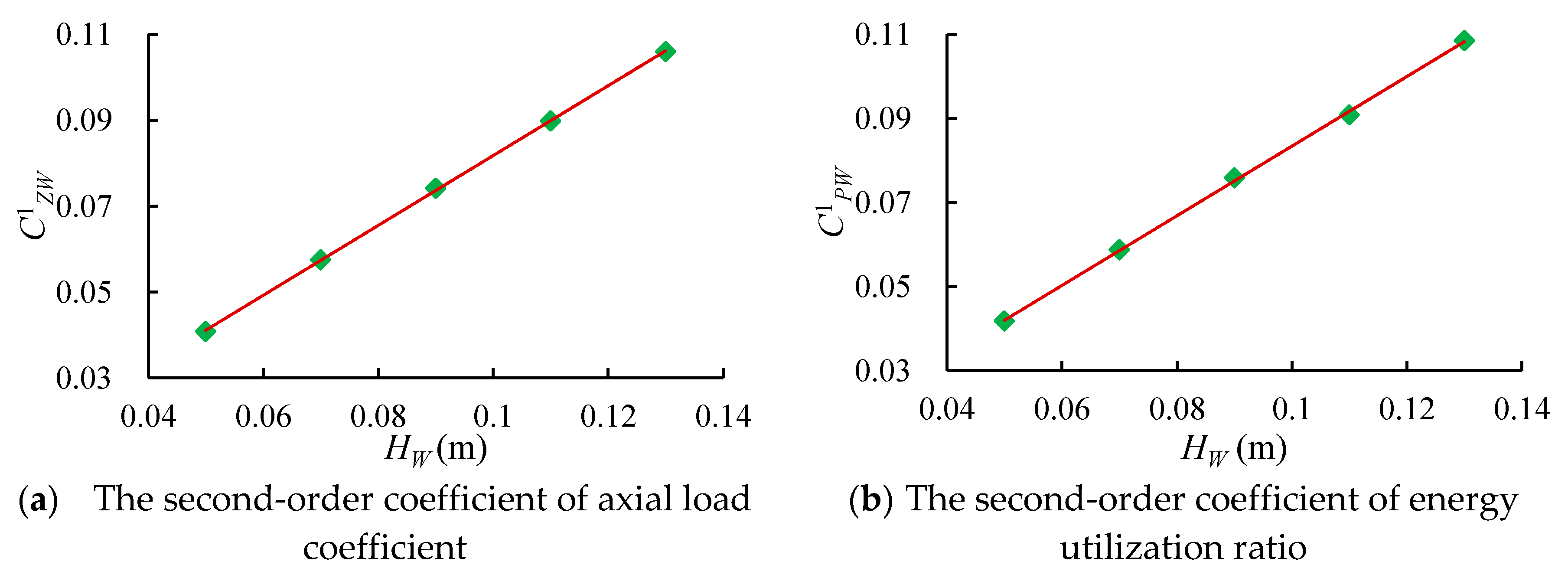
When wave height increased, the average values of axial load coefficients and energy utilization ratios hardly changed. The influence of the second-order term coefficient ($C_{ZT}^2$, $C_{ZW}^2$, $C_{PT}^2$, $C_{PW}^2$) was neglected. The fluctuation amplitudes ($C_{ZT}^1$ and $C_{PT}^1$) based on the rotation frequency of the turbine hardly changed when wave height increased, while the fluctuation amplitudes ($C_{ZW}^1$ and $C_{PW}^1$) based on the wave frequency increased when wave height increased. Figure 11 shows the variation curve of $C_{ZW}^1$ and $C_{PW}^1$ with wave height. $C_{ZW}^1$ and $C_{PW}^1$ increased linearly with wave heights.

5. Conclusions

In this paper, the hydrodynamic loads of a horizontal turbine under wave-flow condition were numerically calculated based on the CFD method. The research conclusions can be summarized as follows:

(1) Under the condition of wave flow, the instantaneous values of axial load coefficients and energy utilization ratios of the turbine produced multi-frequency fluctuations based on wave and rotation frequencies. The fluctuation amplitude based on wave frequency was obviously greater than those based on rotation frequency.

(2) With the increase of the blade tip immersion depth, the time-mean values of the axial load coefficients and energy utilization ratios gradually increased, but the increasing rates decreased. The fluctuation amplitude based on the wave and rotation frequencies both decreased rapidly.

(3) When the wave period increased, the time-mean values of axial load coefficients and energy utilization ratios hardly changed. The fluctuation amplitudes based on the rotation frequency hardly changed when the wave period increased, while the fluctuation amplitudes based on the wave frequency basically increased linearly.

(4) When wave height increased, the time-mean values of axial load coefficients, energy utilization ratios, and the fluctuation amplitudes based on rotation frequency, hardly changed and no obvious rules were found. The fluctuation amplitudes based on the wave frequency increased linearly when wave height increased.

References

- The Crown Estate. UK Wave and Tidal Key Resource Areas Project—Summary Report. Tech. Rep. 2012. Available online: http://www.marineenergywales.co.uk/wp-content/uploads/2016/01/Summary-Report-FINAL.pdf (accessed on 19 June 2020).
- Liu, H.W.; Ma, S.; Li, W.; Gu, H.G.; Lin, Y.G.; Sun, X.J. A review on the development of tidal current energy in China. Renew. Sustain. Energy Rev. 2011, 15, 1141–1146. [Google Scholar] [CrossRef]
- Wang, S.; Zhang, L.; Xu, G.; Zhu, R. Hydrodynamic analysis of a tidal current impeller in a horizontal axis under the condition of a free surface. J. Harbin Eng. Univ. 2016, 37, 1330–1334. [Google Scholar]
- Laß, A.; Schilling, M.; Kumar, J.; Wurm, F.-H. Rotor dynamic analysis of a tidal turbine considering fluid-structure interaction under shear flow and waves. Int. J. Nav. Archit. Ocean Eng. 2019, 11, 154–164. [Google Scholar] [CrossRef]
- Milne, I.A.; Day, A.H.; Sharma, R.N.; Flay, R.G.J. Blade loading on tidal turbines for uniform unsteady flow. Renew. Energy 2015, 77, 338–350. [Google Scholar] [CrossRef] [Green Version]
- Guo, X.; Yang, J.; Lu, W.; Li, X. Dynamic responses of a floating tidal turbine with 6-DOF prescribed floater motions. Ocean Eng. 2018, 165, 426–437. [Google Scholar] [CrossRef]
- Yan, J.; Deng, X.; Korobenko, A.; Bazilevs, Y. Free-surface flow modeling and simulation of horizontal-axis tidal-stream turbines. Comput. Fluids 2017, 158, 157–166. [Google Scholar] [CrossRef]
- Scarlett, G.T.; Viola, I.M. Unsteady hydrodynamics of tidal turbine blades. Renew. Energy 2020, 146, 843–855. [Google Scholar] [CrossRef]
- Barltrop, N.; Varyani, K.S.; Grant, A.; Clelland, D.; Pham, X.P. Investigation into wave current interactions in marine current turbines. Proc. Inst. Mech. Eng. Part A J. Power Energy 2007, 221, 233–242. [Google Scholar] [CrossRef]
- Galloway, P.W.; Myers, L.E.; Bahaj, A.S. Studies of scale turbine in close proximity to waves. In Proceedings of the 3rd International Conference on Ocean Energy, Bilbao, Spain, 5–7 October 2010; pp. 1–6. [Google Scholar]
- Gaurier, B.; Davies, P.; Deuff, A.; Germain, G. Flume tank characterization of marine current turbine blade behaviour undercurrent and wave loading. Renew. Energy 2013, 59, 1–12. [Google Scholar] [CrossRef] [Green Version]
- Henriques, T.A.d.; Tedds, S.C.; Botsari, A.; Najafian, G.; Hedges, T.S.; Sutcliffe, C.J.; Owen, I.; Poole, R.J. The effects of wave–current interaction on the performance of a model horizontal axis tidal turbine. Mar. Energy 2014, 8, 17–35. [Google Scholar] [CrossRef]
- Lust, E.E.; Luznik, L.; Flack, K.A.; Walkerac, J.M.; van Benthem, M.C. The influence of surface gravity waves on marine current turbine performance. Mar. Energy 2014, 3, 27–40. [Google Scholar] [CrossRef]
- Galloway, P.W.; Myers, L.E.; Bahaj, A.S. Quantifying wave and yaw effects on a scale tidal stream turbine. Renew. Energy 2014, 63, 297–307. [Google Scholar] [CrossRef]
- Tutar, M.; Veci, I. Performance analysis of a horizontal axis 3-bladed Savonius type wave turbine in an experimental wave flume (EWF). Renew. Energy 2016, 86, 8–25. [Google Scholar] [CrossRef]
- Zhang, J.; Zhang, J.; Wang, R.; Gu, J.; Lin, X. Investigation on the hydrodynamics around a tidal stream turbine of horizontal axis under the combined action of wave and current. J. Hohai Univ. (Nat. Sci.) 2019, 47, 175–182. [Google Scholar]
- Guo, X.; Yang, J.; Gao, Z.; Moan, T.; Lu, H. The surface wave effects on the performance and the loading of a tidal turbine. Ocean Eng. 2018, 156, 120–134. [Google Scholar] [CrossRef]
- Draycott, S.; Payne, G.; Steynor, J.; Nambiar, A.; Sellar, B.; Venugopal, V. An experimental investigation into nonlinear wave loading on horizontal axis tidal turbines. J. Fluids Struct. 2019, 84, 199–217. [Google Scholar] [CrossRef]
- Wang, S.-q.; Cui, J.; Ye, R.; Chen, Z.-f.; Zhang, L. Study of the Hydrodynamic Performance Prediction Method for a Horizontal-Axis Tidal Current Turbine with Coupled Rotation and Surging Motion. Renew. Energy 2019, 135, 313–325. [Google Scholar] [CrossRef]
- Wang, S.; Xiao, G.; Zhang, L.; Jing, F.-m. The supporting column influence analysis of Horizontal axis tidal current turbine. J. Huazhong Univ. Sci. Technol. Nat. Sci. Ed. 2014, 42, 81–85. [Google Scholar]
- Sufian, S.F.; Li, M.; O’Connor, B.A. 3D modelling of impacts from waves on tidal turbine wake characteristics and energy output. Renew Energy 2017, 114, 308–322. [Google Scholar] [CrossRef] [Green Version]
- Elhanafi, A. Prediction of regular wave loads on a fixed offshore oscillating water column-wave energy converter using CFD. J. Ocean Eng. Sci. 2016, 1, 268–283. [Google Scholar] [CrossRef] [Green Version]
- Menter, F.R. Two-equation eddy-viscosity turbulence models for engineering applications. AIAA J. 1994, 32, 1598–1605. [Google Scholar] [CrossRef] [Green Version]
- Wang, S.; Ingham, D.B.; Ma, L.; Pourkashanian, M.; Tao, Z. Turbulence modeling of deep dynamic stall at relatively low Reynolds number. J. Fluids Struct. 2012, 33, 191–209. [Google Scholar] [CrossRef]
- Liu, J. Study on Hydrodynamic Characteristics of Horizontal Axis Tidal Current Turbine in Wave; Harbin Engineering University: Harbin, China, 2018; Chapter 4. [Google Scholar]
- Jing, F. Hydrodynamics Study on Innovative Floating Tidal Current Power Station; Harbin Engineering University: Harbin, China, 2013; Chapter 3. [Google Scholar]
Figure 1.
Chord length and pitch distribution with radius.
Figure 2.
Schematic and mesh model.
Figure 3.
Schematic diagram of boundary conditions.
Figure 4.
Comparison between calculated and experimental values.
Figure 5.
Comparison of calculated and theoretical values.
Figure 6.
Time history curves of different tip-immersion.
Figure 7.
Time history curve under different wave periods.
Figure 8.
Time history curves of different wave heights.
Figure 9.
Comparison diagram of the computational fluid dynamics (CFD) calculated value and fitting value.
Figure 10.
The first-order coefficient ( and ) curve with wave frequency.
Figure 11.
The first-order coefficient ( and ) curve with wave height.