Effects of Wavy Leading-Edge Protuberance on Hydrofoil Performance and Its Flow Mechanism

1
School of Mechanical and Aerospace Engineering, Jilin University, Changchun 130022, China
2
State Key Laboratory of Automotive Simulation and Control, Jilin University, Changchun 130022, China
*
Author to whom correspondence should be addressed.
J. Mar. Sci. Eng. 2021, 9(10), 1138; https://doi.org/10.3390/jmse9101138
Submission received: 11 September 2021
/
Revised: 13 October 2021
/
Accepted: 14 October 2021
/
Published: 17 October 2021
(This article belongs to the Section Ocean Engineering)
Abstract
:This paper examines the effects on a Clark-y three-dimensional hydrofoil of wavy leading-edge protuberances in a quantitative and qualitative way. The simulation is accompanied by a hybrid RANS-LES model in conjunction with Zwart-Gerber–Belamri model. Detailed discussions of the stable no-cavitating, unsteady cavitating flow fields and the control mechanics are involved. The force characteristics, complicated flow behaviors, cavitation–streamwise vortex interactions, and the cavitating flow instability are all presented. The results demonstrate that protuberances acting as vortex generators produce a continuous influx of boundary-layer vorticity, significantly enhancing the momentum transfer of streamwise vortices and therefore improving the hydrodynamics of the hydrofoil. Significant interactions are described, including the encouragement impact of cavitation evolution on the fragmentation of streamwise vorticities as well as the compartmentation effect of streamwise vorticities binding the cavitation inception inside the troughs. The variations in cavitation pressure are mainly due to the acceleration in steam volume. In summary, it is vital for new hydrofoils or propeller designs to understand in depth the effects of leading-edge protuberances on flow control.
1. Introduction
The traditional hydrofoil, because of its fundamental cross section form of many liquid machinery such as propeller, pump, turbine and undersea, is confronting developments in terms of giant capacity and high speed. When fluid flows past it, a boundary layer with coherent structures forms on the blade surface. It is prone to cavitation corrosion, wall damage, vibration and noise during long term high-speed operations, which significantly impacts security and stability. The coherent structures are intended to be changed such that these unfavorable turbulence effects are effectively controlled [1]. The connection between engineering and biology is now experiencing enormous cognitive shifts. Nature is regarded as a blueprint for improving the performance of mechanical equipment and developing brand-new technologies. Biological inspiration and bionics are attempts to create engineering systems that have characteristics or functions comparable to living system [2].
The great capacity of the aquatic creatures in the environment, extensively utilized as the references for many current underwater vehicles, has been developed [3,4]. Unlike other whales (such as the blue, fin, and minke), which feed by swimming swiftly forward and swallowing food-laden water, the humpback whale relies on pectoral flippers with specialized protuberances (Figure 1a) to readily conduct water acrobatic movements to grab prey [5,6]. Then, from biology to hydrodynamics, the study perspective has changed. Protuberances, as a bionic passive flow control means, can increase hydrodynamic performance while eliminating complex, expensive and demanding maintenance. Conventional wings with straight leading-edges produce flow behaviors with performance limitations due to the co-varying features of lift, drag, and stall. However, simply a little alteration in hydrofoil geometric form (Figure 1b) can provide appealing flow phenomena without additional equipment, or any other material.
The study of protuberance flow mechanisms can help us better understand their impact on more complicated control surfaces. Miklosovic et al. [7] used wind tunnel experiments to determine the force parameters of humpback whale flipper models. They indicated that the inclusion of leading-edge protuberances could lead to a 6% increase in lift and a 40% delay in stall angle of attack (AOA) compared to the baseline model. Following that, Pedro and Kobayashi [8] numerically calculated the flow through a scalloped flipper model at α = 15° and a Reynolds number (Re) of 5 × 10⁵. Their findings revealed that the separating lines around the tip of the flipper were noticeably decreased. Johari et al. [9] performed the effects of various protuberance amplitudes and wavelengths on the flow separation behaviors of a full-span NACA634-021 foil through water tunnel experiments with Re = 1.8 × 10⁵. Flow visualizations using tufts showed that flow separations develop mostly in the trough regions between neighboring protuberances at the leading-edge. According to their conclusions, the wavelength of the protuberances was of minor influence in the force coefficients. The effects of sinusoidal leading-edge modifications on NACA 0021 and NACA 65-021 foils at Re = 1.2 × 10⁵ were assessed by Hansen et al. [10]. They found that protuberances with larger amplitude outperforms in the post-stall regime and proposed that the protuberances functioned similarly to a typical vortex generator. Wei et al. [11] used particle image velocity (PIV) measurements and particle streak photography to investigate the flow behaviors around NACA634-021 hydrofoils with leading-edge protuberances at low Re = 1.4 × 10⁴, revealing that flow separation size is larger along the trough region and smaller in the peak region than the unmodified hydrofoil.
A variety of researches have offered significant insights into the flow control mechanism activated by the presence of protuberances. The most widely recognized hypothesis holds that increasing momentum exchange with streamwise vortices generated by protuberances leads to separation delay, as seen in Figure 1c. Rostamzadeh et al. [12] numerically investigated the counter-rotating primary and secondary vortices over full-span modified foils based on the NACA 0021 profile, which worked synergistically to reduce flow separation and increasing the post-stall lift. Hansen et al. [13] examined the generation and development of the streamwise vortices. In their investigations, a horseshoe-shaped separation zone bounded by a canopy of boundary-layer vorticity was visible behind a protuberance trough, which leaded to a circulation increase of the primary vortices downstream by a continuous influx. Cai et al. [14] emphasized that the streamwise vortices past each protuberance were periodic and symmetric at small angles of attack (AOAs), resulting in a net upwash in tough regions and a net downwash in the peak regions. Hence, there are a longer attachment around the peaks and a larger separation along the toughs. There was therefore a longer flow attachment around the peaks and a larger flow separation along the toughs.
Previous researches have unilaterally focused on the effects of wavy leading-edge on the separation control of non-cavitating flows. It must be pointed out that cavitation is a difficult challenge to tackle for underwater applications [15]. In the presence of cavitation, significant detrimental effects, such as loss efficiency, vibration, noise and material damage, are produced on hydrodynamic performances of the hydraulic machinery [16,17]. Hence, studying the dynamic properties of cavitating flow around hydrofoils with leading-edge protuberances has significant practical importance. Weber et al. [18] conducted experiments to determine the development of cavitation on rudders with wavy leading-edges at low to moderate Res. They observed that the protuberances altered the position of the cavities, which were concentrated in the troughs rather than throughout the whole leading-edge of the smooth rudder. Shi et al. [19] used high-speed photography to capture still pictures around modified blades of a tidal turbine. They also found that the cloud cavity past the protuberances was confined to the troughs, resulting in considerably decreased cavitation extent and intermittent cavitation. Custodio et al. [20] investigated the static cavitation performances of modified hydrofoils, finding that cavitation appeared at the wavy leading-edge at a lower α than the baseline counterparts for a given static pressure. Meanwhile, the cavitation extent of the bigger amplitude hydrofoils is evidently lower. Although the static cavitation properties of hydrofoils with wavy leading-edge have been well described, few researches on their dynamic behaviors have been published. In addition, the interaction between the cavity evolution and streamwise vortices induced by wavy leading-edge is relatively unexplored. Furthermore, it is relatively unknown to interaction between cavity evolution and streamwise vortices generated by wavy leading-edge.
Experimental investigations on cavitation are intuitive, however expensive and disturbed by many factors. Numerical studies on unsteady cavitation have increasingly been prominent in the academic sector with the rapid improvement of computer performance. Turbulence models are essential for analyzing high Re cavitating flows. Although the Reynolds-averaged Navier–Stokes (RANS) equation is widely used in turbulent flow calculations due to its robustness and low calculation cost, an inherent defect must be highlighted: its over-prediction of turbulent viscosity underestimates cavitation instability, resulting in unrealistic cloud cavity shedding [21]. This difficulty was dealt with by several attempts such as a density corrected model (DCM) [22], a filter-based model (FBM) [23], a partially averaged Navier–Stokes model (PANS) [24], and a filter-based density correction model (FBDCM) [25,26]. Although the cloud cavitation may be viewed in a complete shedding, some specific physics associated with turbulent fluctuations are still not adequately replicated. Large eddy simulation (LES), on the other hand, may provide rather accurate results for unstable unsteady cavitating flows by simulating small-scale structures through a filtering process. However, as the mainstream structures become extremely small, high computational power requirements equivalent to the direct numerical simulation (DNS) limits its practical applications. Consequently, hybrid RANS–LES models are naturally available. An integration of both methods, which executes RANS in equilibrium and stable boundary layers near the wall-bounded region while switching to LES in the mainstream sections of interest away from the wall, is thus utilized to improve the capability to the extremely unsteady cavitating flows [27,28].
The primary purpose of the current paper is to evaluate the effects of wavy leading -edge protuberances on hydrodynamic forces and cavitation characteristics of the traditional Clark-y hydrofoil used in water machinery, since the experimental results of unsteady cavitation flow are plentiful. The non-cavitating flow field is examined firstly in this framework to evaluate the law of lift–drag characteristic variation, pressure distribution, and unique vortex formations. The transient cavitation evolution is then studied, and the interaction between cavity pattern and streamwise vortices is obtained in detail. Finally, the physical mechanism of the pressure fluctuations caused by the cavity volume pulsations is examined. For comparison, the flow around the baseline hydrofoil is also presented. As a result, an in-depth understanding of the effects of leading-edge protuberances on flow control is required for the design of new hydrofoils or propellers. For example (Figure 1d), noise levels of the turbines with protuberances are effectively reduced due to a lesser extent of cloud cavitation, which may contribute to the mute and stealth of the submarine [19]. Furthermore, added protuberances on flaps and slots may avoid stall during take-off and landing, as well as save fuel expenditures by removing the control surfaces [29].
2. Numerical Models
2.1. Governing Equations and Turbulence Model
The homogeneous equilibrium medium hypothesis is used to simplify the vapor–water two-phase flow, which assumes that the fluid comments share the common pressure and velocity. The transportations of continuity and momentum are described as follows:
where is the density, μ is viscosity, p is the local pressure, -, - are the velocity components, and α is the volume fraction, E is the element energy, λ is the coefficient of heat conductivity, T is the temperature, h and J are the enthalpy component and the diffusion flux component, respectively, τ is the viscous stress tensor, and - is the viscous dissipation term. Moreover, the subscripts m, l, and v represent the values of mixture, liquid and vapor, respectively.
It has been reported that the high turbulent viscosity of RANS model leads to the underproduction of cavity shedding. Hence, a hybrid RANS–LES turbulence model, namely stress-blended eddy simulation (SBES) [30], is adopted to solve the turbulent flow. Its original concept is that the shear stress transport (SST) k-ω model [31] is applied inside the wall boundary layer flow of equilibrium and stable to reduce calculation effort, while the dynamic LES model [32] is used in the massive separation region to capture turbulence structures. The introduction of a shielding function (-) is the solution to an explicit conversion between the two different models. Then, k equation of the SST k-ω model is given by:
where is the turbulent length, denotes the maximum edge length of the local cell. Within SBES model, the switch between RANS and LES is determined by the following criterion:
To make a rapid transition from the RANS to LES, the coefficient CSBES is usually taken as 0.4. The modified turbulent viscosity is improved as follows:
where a and b are equal to 0.44 and 0.083, respectively, CLES is a coefficient in the dynamic LES model, and Sr means the strain rate. Then the turbulence stress tensor can be defined by continuously mixing the RANS and LES formulations as:
2.2. Cavitaiton Model
Zwart–Gerber–Belamri model [33] is used to simulate the mass transfer process between the occurrence and collapse of the cavitating flow, which has been validated in various cases [34,35]. The phase transition rate is governed by:
where Sevap and Scond represent the mass transfer rates of evaporation and condensation processes, respectively. They are given as follows:
where, Cevap is the evaporation coefficient for vapor generated form the liquid when the local pressure drops below the saturated pressure. Conversely, Ccond is the condensation coefficient for re-conversion of vapor back into liquid when the local pressure exceeds the saturated pressure. In ANSYS FLUENT software, these assumed model constants are αnuc = 5 × 10⁻⁴, Rb = 10−6 m, Cevap = 50 and Ccond = 0.01.
3. Numerical Setup and Solution Details
3.1. Hydrofoil Geometry
The protuberance structures chosen from the humpback whale’s pectoral flippers are employed as biological prototypes for bioinspired hydrofoils, as seen in Figure 1a. According to the literatures [5,9], humpback whales have protuberances on their pectoral flippers with a spanwise range of 10–50% of the chord length and an amplitude of 2.5–12% of the chord length, respectively. Considering the complexity of the morphology and kinematics of actual flippers cannot be effectively represented by numerical analysis, the simplified geometry of the baseline hydrofoil is modified with sinusoidal protuberances.
The baseline hydrofoil has a symmetric Clark-y section with a chord length C = 0.07 m [36]. Figure 1b depicted the section feature of the modified hydrofoil. The origin of a Cartesian coordinate system was initially defined as being at the lower end of the mean leading-edge, X-direction was distributed along the chord, Y-direction was determined by the right-hand law, and the Z-direction was in the span. The wavelength L and the amplitude Am defined the shape of the leading-edge protuberances. The following equation therefore determined the leading-edge locations:
To maintain the position of maximum thickness and the profile behind maximum thickness point (), a nonlinear shearing transformation was applied to the cross section of the baseline hydrofoil as:
where X and X1 were the abscissas of the baseline and modified hydrofoils, respectively. The first derivative of Equation (13) was described as:
It maintained the leading-edge radius of the baseline hydrofoil and achieved a continuous curvature radius of the cross sections behind the maximum thickness point. This work analyzed two protuberance wavelengths L = 0.1C and 0.15C together with two amplitudes Am = 0.025C and 0.04C, as shown in Figure 2a. These wavelengths and amplitudes were within the range of relevant values of the humpback whale’s pectoral flippers, resulting in a not-too-sharp head waveform. Through controlling the coherent structures of the boundary layer, we intended to mitigate the flow separation while also weakening the cavitation scale.
3.2. Mesh Layout and Solution Setup
The computational domain and boundary conditions were shown in Figure 2b. It should be pointed out that considering the high computational costs of the real spanwise size in the experiment, the span width was usually chosen as twice the thickness of the hydrofoil to resolve the streamwise vortices [37,38]. Therefore, a compromised span width was chosen as 0.3C in the current study, which had been validated by many researchers [35,38,39,40]. Note that a periodic condition was arranged on the side wall to analyze the fundamental interaction of the turbulent vortex structures [38,39,41]. The inlet velocity was set to U∞ = 10 m/s and the out pressure Pout was determined by the cavitation number (σ). All other boundary conditions were imposed as no-slip walls. Two key dimensionless parameters: Reynolds number (Re) and cavitation number (σ), were defined as:
The present calculation applied a finite volume method, i.e., ANSYS FLUENT, to simplify the multiphase system to a homogeneous flow. In the non-cavitating case, the steady state solver was adopted due to the unnecessary time discretization. In the cavitating case, the SIMPLEC-type pressure velocity coupling correction method was employed to improve the convergence and calculating speed. Bounded central differencing and PRESTO discretization schemes were used for momentum and pressure transport equations, respectively. The second-order upwind scheme was applied to other convective phases. A maximum of 25 iterations was used in each loop to achieve a tradeoff between the computational efficiency and accuracy. The convergence criteria of all equations were set at a residual target of 10−5, which were sufficient for the current transient simulation. In the current work, the time step Δt = 2 × 10⁻⁵ s was used to acquire complicated features, as recommended by Liu et al. [28].
To confirm the grid dependency, four grid layouts were created, with the only change being the node numbers (i.e., 15, 30, 60, 90) in the spanwise direction. For four cases, the mid-span grid distribution was the same for accurately capturing the boundary layers. The grid scheme was validated by an analysis of the lift coefficients (Cl) and drag coefficient (Cd) under non-cavitation at AOA = 8° according to existing test data of the baseline hydrofoil [36]. The force coefficients were as follows:
Figure 3 showed that the force coefficients stayed essentially unchanged in the latter two cases. To save computing costs, the medium grid with 60 spanwise nodes was thereby used as the final mesh. In addition, compared with the experimental measurements (Cl0 = 1.152 and Cd0 = 0.037), the calculated lift and drag coefficients of the baseline hydrofoil were Cl = 1.190 and Cd = 0.039, respectively, indicating that the current grid satisfied the calculation accuracy requirements.
The Grid Convergence Index (GCI) approach, proposed by Celik et al. [42], was also used to estimate discretization errors. Taking into account the lift coefficient as the key variable as listed in Table 1, it was shown that the numerical uncertainty was less than 3%. Hence, it was confirmed that the current mesh resolution was reliable for subsequent simulations.
4. Results and Discussion
4.1. Non-Cavitating Flow
Figure 4 depicted Cl and Cd computed at various AOAs, with an emphasis on the hydrodynamic characteristics of the baseline and modified hydrofoils. For the baseline hydrofoil, the Cl grew approximately linearly from AOA = 0–10°, and the stall occurred at 15° with an abrupt loss of lift and substantial increases in drag. However, the Cl profiles of the modified hydrofoils rose with lower slopes before a decrease around 10°. They then maintained sustained growth after 15°, indicating a stronger post-stall feature. For the Cd profiles of the baseline hydrofoil, a sharp increase was observed after 10°. However, it displayed a linear continuous increase from 10° to 25° in modified hydrofoils. The lift-to-drag ratio Cl/Cd profiles demonstrated that the baseline hydrofoil performed better at 5° < AOA < 20° owing to the high Cl. The maximum Cl/Cd of Type I and II at AOA = 5° were 1.81% and 2.97% higher than that of the baseline, respectively, whereas Type III had an 11.16% drop due to a larger Cd.
As a result, increasing the wavelength or amplitude of the protuberances arbitrarily might degrade hydrodynamic performance. Overall, Type II performed somewhat better than the other two modified versions. These findings also assist to explain why humpbacks with tubercles on their pectoral flippers can have such great agility.
The numerical findings were shown next for the sake of understanding of the flow separation delay. Figure 5 illustrated simulated velocity distributions around the leading edge in the XY plane. At low AOA = 8°, the introduction of protuberances alleviated the trailing edge separation. At low AOA = 25°, the significant difference was that the whole suction surface of the baseline hydrofoil is in a separation condition. However, the flow across wavy leading-edge remained attached within a certain distance and confined the separation extension from the tip region. The separation zones travelled further back in the case of type II and III, producing counter-rotating vortex formations behind. The suppression of this flow separation was strongly connected to hydrodynamic characteristics.
The investigation of force fluctuations along the spanwise was ensured by the analysis of surface pressure characteristics. Figure 6 compared the chordwise pressure coefficients (Cp) over the peak and trough of the modified hydrofoils at AOA = 8° and 25° to the baseline hydrofoil. The title x/C = 0 is on the leading-edge of the hydrofoils, and x/C = 1, on the trailing-edge. At AOA = 8°, the flow remained on the suction side of all the hydrofoils, since the pressure coefficient was gradually increasing from the leading-edge to the trailing edge. The results show that the minimum Cp in the tough region of the modified hydrofoils was much smaller that of the baseline, implying an earlier onset of cavitation. In contrast, a higher minimum Cp of the peak region suggested a reduced cavitation probability. In this case, it was more crucial for the wave amplitude to affect the minimum Cp. At AOA = 25°, the wide separation on the whole suction side could be seen for the baseline hydrofoil as the Cp was almost constant from the leading-edge to the trailing-edge. For the modified hydrofoils, Cp was constant after x/C = 0.16~0.20 along the peak of protuberance, indicating a delay flow separation corresponding to Figure 5. According to the Bernoulli equation, the flow past the trough region would experience a pressure rise during the anticipated stroke, resulting in a larger reverse pressure gradient and a premature flow separation. Due to the low-pressure effect, the Cp of the trough region performed a “small platform” [43]. For the high AOA, the wavelength showed a greater influence on the minimum Cp.
Streamwise vortices mechanism as the most widely accepted hypothesis was used to visualize the flow control mode. The fundamental assumption was that the streamwise vortices induced by the wavy leading edge enhanced the momentum exchange of the boundary layer. The 3D streamlines could directly exhibit the vortex structures on the suction surface of the hydrofoils. In addition, the slides of steamwise vorticity ωx were extracted at different streamwise positions at AOA = 8° to emphasize the existence and intensity of downstream counter-rotating vortices. Figure 7 demonstrated that the mainstream was disturbed by the protuberances, resulting in visible vortex flow in the tailing-edge of the modified hydrofoils. The flow past each protuberance, together with a pair of counter-turning vortices, was essentially symmetric and exhibited a regularity comparable to the prior researches [11,13]. As the flow developed downstream, the area of ωx expended. The region of ωx expends in area as the flow develops downstream. However, the impacted region of Type I was obviously smaller than the other two modifications. It was noticed that the vortex on the left side rotated clockwise, while the one on the right side turned anti-clockwise. These counter-rotating vortices thereby drove flows to diverge along the trough plane, while causing them to converge along the peak plane [44]. As a result of the composite action of the two neighboring vortices, low pressure coefficients and significant unfavorable pressure gradients occurred at the trough regions, producing early flow separations.
4.2. Cloud Cavitation Evolution
The interactions between the cavitation and the steamwise vortices were examined by the transient behaviors and cavity patterns. Results were presented for the hydrofoils fixed at α = 8° under cloud cavitating condition (σ = 0.8). Figure 8 plotted the normalized total vapor volume V of the four hydrofoils against two typical periods, which was defined as:
It was seen that the vapor volume fluctuated quasi-periodically as a result of the generation and shedding of the cavity. The predicted results of the modified hydrofoils presented certain cavitation control abilities, especially the Type II.
Figure 9 and Figure 10 showed the transient behavior of the predicted cavitating flow using six typical snapshots in one classic cycle. To provide a vivid insight into the physical mechanism of the cavitation evolution, the 3D iso-surface of the cavity was shown in Figure 9. It was show that the distinct quasi-periodic patterns of the numerical cavity morphologies were contrasted with experiment findings of the baseline hydrofoil [45]. The flow direction and vortex movement in the cavity were depicted by the black arrows.
In the streamwise direction, the transient flow characteristics around the baseline and modified hydrofoils were comparable. At t1 = 0.125 Tcycle, the transparent attached cavity grew continuously from the leading-edge, and its behavior appeared relatively stable until the anti-clockwise cavitation vortex and re-entrant jet flow emerged in the trailing-edge at t3 = 0.475 Tcycle. During this process, the attached cavity of the baseline hydrofoil reached nearly to the whole suction side, and the large vapor could from the breakup of the preceding sheet cavity still remained in the trailing-edge. The length of the sheet cavity and the scale of the cloud cavity were both diminished in different degrees in respect of the modified hydrofoils. Following that, the re-entrant jet flow collided with the main flow, rose upward, and then destroyed the cavity interface between t4 = 0.625 Tcycle and t5 = 0.875 Tcycle. At the rear of the hydrofoil, the sheet cavity partially split and there was a new cloud cavity. Finally, at t5 = 1.000 Tcycle, a newly attached sheet cavity continued to periodically form at the leading-edge, while the shedding cloud cavity gradually lifted up from the wall and collapsed downstream in the next cycle. The numerical model described the transient cavity features well.
In Figure 10, the mid-span of the baseline hydrofoil, the mid-spans of the trough and the peak of the Type I hydrofoil were selected to examine the differences in transient cavity behaviors along the streamwise direction. Notably, the inception of sheet cavity was only detected in the leading-edge troughs, whereas peak regions had practically no cavitation bubbles. It was assumed to be caused by the modified hydrofoils’ unique spanwise Cp distribution, as illustrated in Figure 6. Relatively thin sheet cavity developed from the stable low-pressure region. For the baseline hydrofoil, the spanwise distribution of the sheet cavity at the leading-edge was nearly homogeneous. This behavior was also consistent with other experimental findings [20]. Furthermore, the presence of the counter-rotating vortices disturbed the flow field following the protuberances, and enhanced the momentum of boundary layer. As a consequence, the modified hydrofoils were able to resist the large adverse pressure gradient, which weakened the chordwise development of the cavity and considerably reduced its scale compared to the baseline hydrofoil. The pressure gradient distribution on the X-direction was also presented in Figure 10, to further explain the difference in the behaviors of cavity development between the two hydrofoils and to further highlight the mechanism of cavitation shedding. The negative pressure gradient at the leading-edge promoted the growth and convection of the sheet cavity. At t3 = 0.475 Tcycle, a flow separation in closure region produced a change in the pressure gradient at the rear of the hydrofoil, leading in the development of a re-entrant jet that ruptured the vapor-liquid interface. From t4 = 0.625 Tcycle to t6 = 1.000 Tcycle, it was obvious that there was a negative pressure gradient in front of the split cavity and a positive pressure gradient behind it, which would cause the cloud vapor to rotate. Meanwhile, a significant high-pressure gradient formed near the trailing-edge, indicating a pressure fluctuation in this region and a possibility for surface erosion. Hence, one advantage of the modified hydrofoil was that it decreased the pressure gradient at the trailing-edge, thus shrinking the shedding cavity, and reducing the negative impact of vibration on operating performance.
To better visualize the vortex structures during the cavity shedding process, Figure 11 depicted the iso-surfaces of velocity based in the Q-criterion (Q = 2 × 10⁴ s−2) for the baseline and Type I hydrofoils. The variable is defined as follows:
where Ωij denotes the vorticity tensor, Sij denotes the rate of the strain tensor. Note that the positive value of this variable reveals vortex regions where the rotation of flow overcomes the strain. It was observed that the cavitating vortex structures had a close relationship with the cavity shape, which also evolved quasi-periodically. The large scale of the shedding cloud cavity led to more complex vortex structures. As a result, it was clear that the scale of the vortex structures on the baseline hydrofoil was larger than that of the Type I hydrofoil, particularly during the cavity shedding process. Furthermore, the spanwise distribution of velocity along the leading edge of the Type I hydrofoil demonstrated the flow accelerated in the troughs and decelerated in the peaks.
4.3. Interactions between Streamwise Vortices and Cavitation
In Figure 12, the iso-surfaces of ωx = ±200 under the non-cavitating and cavitating flows were given to provide an intuitive description of the variations of the streamwise vortices after cavitation. For non-cavitation, the primary streamwise vortices existed at x/C = 0.2 plane and the secondary streamwise vortices formed from roughly x/C = 0.7 plane, thus these two planes as well as x/C = 0.4 plane were examined immediately. According to the previous studies [12,46], there would be a downwash velocity component in the peak and an upwash velocity component in the though due to the counter-rotating vortices. Based on the Prandtl lifting line theory, the downwash velocity component could lower the local effective AOA, resulting in a higher Cp in the peak at the leading-edge as shown in Figure 6. The upwash velocity could instead increase the local effective α, resulting in a lower Cp in the trough as compared to the baseline hydrofoil. Furthermore, it was evident that there were disordered and mixed vortices formed after the x/C = 0.2, indicating that no effective upwash or downwash was induced in the cavitation regions.
To investigate the influence of protuberances on the process of streamwise vortex formation under cavitation, the vorticity transport equation in the variable density flow field was extracted at different YZ planes as follows:
The first part on the right side of Equation (21) was the vortex stretching term, which reflected the stretching and tilting of a vortex caused by the velocity gradients. The second part, referred to as the vortex dilatation term, described the expansion and contraction of fluids that could reflect the fluid compressibility. The next part was the baroclinic torque term, which was caused by the imbalance between the density and pressure gradients. The last term, namely the viscous diffusion term, was usually negligible in the fully developed turbulence [45]; so, it was then omitted.
Figure 13 showed that the sheet cavity developed steadily from the leading-edge at the x/C = 0.2 plane. It was seen that the vapor distribution decreased significantly downstream of the peaks. Here, the first three decomposition terms of the vorticity were symmetrical with the vapor distribution along the trough centerline, and the primary streamwise vortices began to partially break up. Actually, water was considered to be incompressible in the region without cavitation [47]. So, the values of the vortex dilatation and baroclinic torque terms were equal to zero at the x/C = 0.4 plane, and only the stretch term played an important role. At the x/C = 0.7 plane, there was a rather large-scale cloud cavity with irregular shape. As a result of the destroyed spanwise pressure gradient, the secondary streamwise vortices could not develop in an ordered manner equivalent to the non-cavitation condition. At the same time, the distributions of the three decomposition terms were obviously disordered due to the non-uniform and violent flow in the cloud cavity. The vortex stretching term was particularly noteworthy due to the abrupt shift in the size and direction of the vorticity caused by the non-uniform velocity.
4.4. One Dimensional Analysis Method of Cavitating Flow Instability
Strong instability caused by the cavity shedding will cause severe vibrations, which are not permitted during the safe operation of hydraulic machinery. A simplified one-dimensional model was calibrated using the Type II findings to readily evaluate the instantaneous variations of the present cavitating flow, as illustrated in Figure 14. It was assumed that there was a cavity with volume V on the suction surface, and the liquid phase was incompressible [48]. Then the flow continuity equation was given by the variations of flow rate between inlet and outlet boundaries:
where the inlet flow rate Qin and outlet pressure Pout were constants. The outlet flow rate Qout varied as cavity volume changed. According to Bernoulli equation, the following result was obtained without considering the head loss in the channel:
To avoid the influence of the cavity wake, the point was placed at the position of x/C = 0.5 on the pressure side rather than the suction side. Combining the Equations (26) and (27), we obtained:
The above equation stated clearly that pressure fluctuation was proportional to the second derivative of the cavity volume.
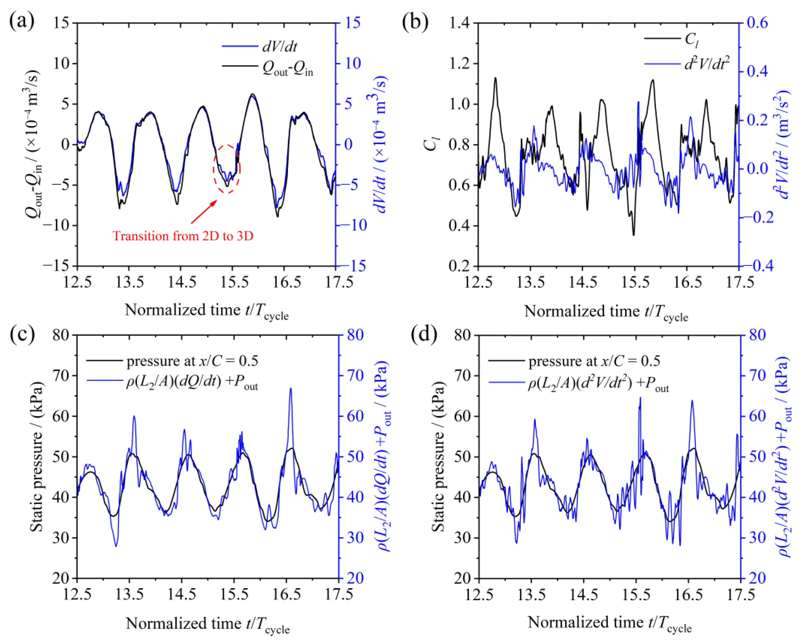
As shown in Figure 15a, the flow rate difference Qout − Qin was highly correlated with the first derivative of the cavity volume dV/dt, indicating the numerical result could accurately obtain time-varying characteristics throughout the quasi-periodic cavity evolution. However, it was worth noting that the numerical simulation underestimated the fluctuation of the flow difference, as marked by a red circle, which corresponded to the period of cavity shedding. At this stage, the shedding vapor cloud had undergone a transition from 2D to 3D, which was also reported by Chen et al. [49] and Ji et al. [38]. Figure 15b demonstrated that the numerical lift coefficient Cl had a positive coherence with the second derivative of cavity volume d2V/d2t (i.e., the acceleration of cavity volume), indicating that the force characteristics of the hydrofoil surface were obviously dominated by the local cavity motions [50]. Figure 15c showed that the pressure fluctuations at the numeric model monitoring point matched the evaluation result derived from Bernoulli equation. The amplitude predicted by Equation (27) of the fluctuation pressure was nonetheless substantially greater, which might be caused by the violent impact of the cavity evolution. Accordingly, the second derivative of total cavity volume agreed well with the pressure fluctuations as plotted in Figure 15d. To a certain extent, there was a quantitative description of the relationship between the cavity shape and cavitation exciting force. It was concluded that the acceleration of the cavity volume played a crucial role on the pressure fluctuations around the hydrofoil. As a result, controlling the cavity volume acceleration might be a new potential approach for reducing the detrimental effect of pressure fluctuations in cavitation.
5. Conclusions
In this work, the inclusion of flipper protuberances on the leading edge was demonstrated to have a substantial influence on the hydrodynamic performance and cavitation characteristics of the hydrofoils. It can mitigate flow separation while also weakening the cavitation scale as an encouraging passive technique of altering fluid flow. As a result, this application offers promise in the design of propellers, turbines, wings, and so on. The major findings given here can be summarized as follows:
(1) The wavy leading edge is proven to effectively control flow separation. In comparison to the baseline hydrofoil, the modified hydrofoils exhibit inferior hydrodynamic performances inside the pre-stall region, but higher Cl and lower Cd in the post-stall region. However, raising the amplitude or wavelength arbitrarily may result in poor performance in terms of force characteristics.
(2) Flow visualization illustrates the periodic and symmetric streamwise vortices originating from protuberances are responsible for the hydrodynamics and pressure distributions of the modified hydrofoils. These counter-rotating vortices contribute momentum to the boundary layer, thereby restricting the separation of the leading edge into the trough region.
(3) The cavitation development of the baseline hydrofoil cavitation is consistent with the current references. The sheet cavity is tiny and stable towards the leading edge, while the cloud cavity shedding at the rear is large and unsteady. When it comes to the modified hydrofoils, the location as well as the scale of cavitation are considerably limited by the streamwise vortices. The sheet cavity is cut off spanwise with no cavity detected at the peaks, and it disturbs the downstream flow, which makes the cavitation scale considerably lower than the baseline hydrofoil. The analysis of the vorticity transportation equation demonstrates that the cavitation in turn affects secondary streamwise vortices that are mixed and broken due to the three disordered decomposition terms.
(4) A simplified one-dimensional model is established to analyze the relationship between the pressure fluctuations and the cavity evolution. It indicates that the cavity volume acceleration is mainly responsible for the pressure fluctuation. It can help to control cavitation oscillations in the engineering designs.
In conclusion, this work contributes to deepening the understanding of the flow mechanism of the three-dimensional hydrofoil of wavy leading-edge protuberances. Researchers have concluded that complex mixing of multiple phases near free surfaces may result in ventilation flows in marine system [51]. The numerical prediction of ventilation flows around the hydrofoil will a challenging task in the future work.
Author Contributions
Methodology, J.L.; software, J.L.; writing—original draft preparation, J.L.; formal analysis, C.L.; investigation, C.L.; writing—review and editing, X.L. All authors have read and agreed to the published version of the manuscript.
Funding
This research was funded by the Natural Science Foundation of Jilin Province (Grant No. 20200201222JC), the Graduate Innovation Fund of Jilin University (Grant No. 101832020CX107), the National Natural Science Foundation of China (Grant No. 52075212) and the Fundamental Research Funds for the Central Universities, Jilin University.
Institutional Review Board Statement
Not applicable.
Informed Consent Statement
Not applicable.
Data Availability Statement
The data presented in this study are available on request from the corresponding author.
Conflicts of Interest
The authors declare no conflict of interest.
Nomenclature
| Re | Reynolds number; |
| AOA | angle of attack; |
| mixture’s mass density, kg·m−3; | |
| velocity component in the i direction, m/s; | |
| p | local pressure, Pa; |
| liquid density, kg·m−3; | |
| vapor density, kg·m−3; | |
| turbulent viscosity, Pa·s; | |
| vapor volume fraction; | |
| E | element energy; |
| λ | heat conductivity coefficient; |
| T | temperature; |
| h | enthalpy component; |
| J | diffusion flux component; |
| τ | viscous stress tensor; |
| viscous dissipation term; | |
| turbulence scale; | |
| volume of the cell; | |
| typical grid size; | |
| shielding function coefficient; | |
| Sr | strain rate |
| αnuc | nucleation volume fraction; |
| Rb | radius of a nucleation site; |
| Cevap | evaporation coefficient; |
| Ccond | condensation coefficient; |
| C | chord length, m; |
| L | protuberance wavelength, m; |
| Am | protuberance amplitude, m; |
| inlet velocity, m/s; | |
| Pout | outlet pressure, Pa; |
| σ | cavitation number; |
| time step size, s; | |
| Cl | lift coefficient; |
| Cd | drag coefficient; |
| Cp | pressure coefficient. |
References
- Arai, H.; Doi, Y.; Nakashima, T.; Mutsuda, H. A Study on Stall Delay by Various Wavy Leading Edges. J. Aero Aqua Bio-Mech. 2010, 1, 18–23. [Google Scholar] [CrossRef] [Green Version]
- Woodward, B.L.; Winn, J.P.; Fish, F.E. Morphological specializations of baleen whales associated with hydrodynamic performance and ecological niche. J. Morphol. 2006, 267, 1284–1294. [Google Scholar] [CrossRef] [PubMed]
- Bushnell, D.M.; Moore, K.J. Drag Reduction in Nature. Annu. Rev. Fluid Mech. 1991, 23, 65–79. [Google Scholar] [CrossRef]
- Miklosovic, D.S.; Murray, M.M.; Howle, L.E. Experimental Evaluation of Sinusoidal Leading Edges. J. Aircr. 2007, 44, 1404–1408. [Google Scholar] [CrossRef]
- Fish, F.E.; Battle, J.M. Hydrodynamic design of the humpback whale flipper. J. Morphol. 1995, 225, 51–60. [Google Scholar] [CrossRef] [PubMed]
- Fish, F.; Lauder, G. Passive and active flow control by swimming fishes and mammals. Annu. Rev. Fluid Mech. 2006, 38, 193–224. [Google Scholar] [CrossRef] [Green Version]
- Miklosovic, D.S.; Murray, M.M.; E Howle, L.; E Fish, F. Leading-edge tubercles delay stall on humpback whale (Megaptera novaeangliae) flippers. Phys. Fluids 2004, 16, L39–L42. [Google Scholar] [CrossRef] [Green Version]
- Pedro, H.; Kobayashi, M. Numerical study of stall delay on humpback whale flippers. In Proceedings of the 46th AIAA Aerospace Sciences Meeting and Exhibit, Reno, NV, USA, 7–10 January 2008; p. 0584. [Google Scholar]
- Johari, H.; Henoch, C.; Custodio, D.; Levshin, A. Effects of Leading-Edge Protuberances on Airfoil Performance. AIAA J. 2007, 45, 2634–2642. [Google Scholar] [CrossRef]
- Hansen, K.; Kelso, R.M.; Dally, B. Performance Variations of Leading-Edge Tubercles for Distinct Airfoil Profiles. AIAA J. 2011, 49, 185–194. [Google Scholar] [CrossRef]
- Wei, Z.; New, T.; Cui, Y. An experimental study on flow separation control of hydrofoils with leading-edge tubercles at low Reynolds number. Ocean Eng. 2015, 108, 336–349. [Google Scholar] [CrossRef]
- Rostamzadeh, N.; Hansen, K.; Kelso, R.M.; Dally, B.B. The formation mechanism and impact of streamwise vortices on NACA 0021 airfoil’s performance with undulating leading edge modification. Phys. Fluids 2014, 26, 107101. [Google Scholar] [CrossRef]
- Hansen, K.L.; Rostamzadeh, N.; Kelso, R.M.; Dally, B.B. Evolution of the streamwise vortices generated between leading edge tubercles. J. Fluid Mech. 2016, 788, 730–766. [Google Scholar] [CrossRef]
- Cai, C.; Zuo, Z.; Maeda, T.; Kamada, Y.; Li, Q.; Shimamoto, K.; Liu, S. Periodic and aperiodic flow patterns around an airfoil with leading-edge protuberances. Phys. Fluids 2017, 29, 115110. [Google Scholar] [CrossRef]
- Luo, X.-W.; Ji, B.; Tsujimoto, Y. A review of cavitation in hydraulic machinery. J. Hydrodyn. 2016, 28, 335–358. [Google Scholar] [CrossRef]
- Arndt, R.E.A. Cavitation in Fluid Machinery and Hydraulic Structures. Annu. Rev. Fluid Mech. 1981, 13, 273–326. [Google Scholar] [CrossRef]
- Rus, T.; Dular, M.; Širok, B.; Hočevar, M.; Kern, I. An Investigation of the Relationship between Acoustic Emission, Vibration, Noise, and Cavitation Structures on a Kaplan Turbine. J. Fluids Eng. 2007, 129, 1112–1122. [Google Scholar] [CrossRef]
- Weber, P.W.; Howle, L.E.; Murray, M.M. Lift, Drag, and Cavitation Onset on Rudders with Leading-edge Tubercles. Mar. Technol. SNAME News 2010, 47, 27–36. [Google Scholar] [CrossRef]
- Shi, W.; Atlar, M.; Rosli, R.; Aktas, B.; Norman, R. Cavitation observations and noise measurements of horizontal axis tidal turbines with biomimetic blade leading-edge designs. Ocean Eng. 2016, 121, 143–155. [Google Scholar] [CrossRef] [Green Version]
- Custodio, D.; Henoch, C.; Johari, H. Cavitation on hydrofoils with leading edge protuberances. Ocean Eng. 2018, 162, 196–208. [Google Scholar] [CrossRef]
- Emvin, P.; Davidson, L.; Coutier-Delgosha, O.; Reboud, J.L.; Delannoy, Y. Numerical simulation of the unsteady behaviour of cavitating flows. Int. J. Numer. Methods Fluids 1997, 24, 519–530. [Google Scholar] [CrossRef]
- Coutier-Delgosha, O.; Fortes-Patella, R.; Reboud, J.L. Evaluation of the Turbulence Model Influence on the Numerical Simulations of Unsteady Cavitation. J. Fluids Eng. 2003, 125, 38–45. [Google Scholar] [CrossRef] [Green Version]
- Johansen, S.T.; Wu, J.; Shyy, W. Filter-based unsteady RANS computations. Int. J. Heat Fluid Flow 2004, 25, 10–21. [Google Scholar] [CrossRef]
- Girimaji, S.S.; Jeong, E.; Srinivasan, R. Partially Averaged Navier-Stokes Method for Turbulence: Fixed Point Analysis and Comparison With Unsteady Partially Averaged Navier-Stokes. J. Appl. Mech. 2005, 73, 422–429. [Google Scholar] [CrossRef]
- Huang, B.; Wang, G.-Y.; Zhao, Y. Numerical simulation unsteady cloud cavitating flow with a filter-based density correction model. J. Hydrodyn. 2014, 26, 26–36. [Google Scholar] [CrossRef]
- Roohi, E.; Zahiri, A.P.; Pasandidehfard, M. Numerical simulation of cavitation around a two-dimensional hydrofoil using VOF method and LES turbulence model. Appl. Math. Model. 2013, 37, 6469–6488. [Google Scholar] [CrossRef]
- Liu, C.; Bu, W.; Xu, D.; Lei, Y.; Li, X. Application of Hybrid RANS/LES turbulence models in rotor-stator fluid machinery: A comparative study. Int. J. Numer. Methods Heat Fluid Flow 2017, 27. [Google Scholar] [CrossRef]
- Liu, C.; Yan, Q.; Wood, H.G. Numerical investigation of passive cavitation control using a slot on a three-dimensional hydrofoil. Int. J. Numer. Methods Heat Fluid Flow 2019, 30, 3585–3605. [Google Scholar] [CrossRef]
- Fish, F.E.; Weber, P.W.; Murray, M.M.; Howle, L.E. The Tubercles on Humpback Whales’ Flippers: Application of Bio-Inspired Technology. Integr. Comp. Biol. 2011, 51, 203–213. [Google Scholar] [CrossRef] [PubMed] [Green Version]
- Walters, D.K.; Bhushan, S.; Alam, M.F.; Thompson, D.S. Investigation of a Dynamic Hybrid RANS/LES Modelling Methodology for Finite-Volume CFD Simulations. Flow Turbul. Combust. 2013, 91, 643–667. [Google Scholar] [CrossRef]
- Menter, F.R. Two-equation eddy-viscosity turbulence models for engineering applications. AIAA J. 1994, 32, 1598–1605. [Google Scholar] [CrossRef] [Green Version]
- Germano, M.; Piomelli, U.; Moin, P.; Cabot, W.H. A dynamic subgrid-scale eddy viscosity model. Phys. Fluids A Fluid Dyn. 1991, 3, 1760–1765. [Google Scholar] [CrossRef] [Green Version]
- Zwart, P.; Gerber, A.G.; Belamri, T. A two-phase flow model for predicting cavitation dynamics. In Proceedings of the 5th International Conference on Multiphase Flow, Yokohama, Japan, 30 May–3 June 2004; p. 152. [Google Scholar]
- Morgut, M.; Nobile, E.; Bilus, I. Comparison of mass transfer models for the numerical prediction of sheet cavitation around a hydrofoil. Int. J. Multiph. Flow 2011, 37, 620–626. [Google Scholar] [CrossRef]
- Liu, J.; Yu, J.W.; Yang, Z.L.; He, Z.; Yuan, K.; Guo, Y.H.; Li, Y. Numerical investigation of shedding dynamics of cloud cavitation around 3D hydrofoil using different turbulence models. Eur. J. Mech. B-Fluids 2021, 85, 232–244. [Google Scholar] [CrossRef]
- Huang, B.; Young, Y.L.; Wang, G.Y.; Shyy, W. Combined experimental and computational investigation of unsteady structure of sheet/cloud cavitation. J. Fluids Eng. Trans. ASME 2013, 135, 071301. [Google Scholar] [CrossRef]
- Sagaut, P. Large Eddy Simulation for Incompressible Flows: An Introduction; Springer: New York, NY, USA, 2006. [Google Scholar]
- Ji, B.; Luo, X.W.; Arndt, R.E.A.; Peng, X.X.; Wu, Y.L. Large eddy simulation and theoretical investigations of the transient cavitating vortical flow structure around a NACA66 hydrofoil. Int. J. Multiph. Flow 2015, 68, 121–134. [Google Scholar] [CrossRef] [Green Version]
- Long, Y.; Long, X.P.; Ji, B.; Xing, T. Verification and validation of large eddy simulation of attached cavitating flow around a Clark-Y hydrofoil. Int. J. Multiph. Flow 2019, 115, 93–107. [Google Scholar] [CrossRef]
- Pendar, M.R.; Esmaeilifar, E.; Roohi, E. LES study of unsteady cavitation characteristics of a 3-D hydrofoil with wavy leading edge. Int. J. Multiph. Flow 2020, 132, 103415. [Google Scholar] [CrossRef]
- Lakshmipathy, S.; Girimaji, S.S. Partially averaged Navier–Stokes (PANS) method for turbulence simulations: Flow past a circular cylinder. J. Fluids Eng. Trans. ASME 2010, 132, 121202. [Google Scholar] [CrossRef]
- Celik, I.B.; Ghia, U.; Roache, P.J.; Freitas, C.J. Procedure for estimation and reporting of uncertainty due to discretization in CFD applications. J. Fluids Eng. Trans. ASME 2008, 130, 078001. [Google Scholar]
- Carr, L.W.; Mcalister, K.W.; M Cc Roskey, W.J. Analysis of the Development of Dynamic Stall Based on Oscillating Airfoil Experiments; NASA Technical Reports; Washington, DC, USA, 1977; Available online: https://www.semanticscholar.org/paper/Analysis-of-the-development-of-dynamic-stall-based-Carr-Mcalister/a08a1421e19170b8c93867efdd23781fbd5eb201#citing-papers (accessed on 10 October 2021).
- Zhang, M.M.; Wang, G.F.; Xu, J.Z. Experimental study of flow separation control on a low-Re airfoil using leading-edge protuberance method. Exp. Fluids 2014, 55, 1710. [Google Scholar] [CrossRef]
- Huang, B.; Zhao, Y.; Wang, G.Y. Large Eddy Simulation of turbulent vortex-cavitation interactions in transient sheet/cloud cavitating flows. Comput. Fluids 2014, 92, 113–124. [Google Scholar] [CrossRef]
- Li, Z.H.; Qian, Z.D.; Ji, B. Transient cavitating flow structure and acoustic analysis of a hydrofoil with whalelike wavy leading edge. Appl. Math. Modell. 2020, 85, 60–88. [Google Scholar] [CrossRef]
- Wang, C.C.; Wu, Q.; Huang, B.; Wang, G.Y. Numerical investigation of cavitation vortex dynamics in unsteady cavitating flow with shock wave propagation. Ocean Eng. 2018, 156, 424–434. [Google Scholar] [CrossRef]
- Chen, C.K.; Nicolet, C.; Yonezawa, K.; Farhat, M.; Avellan, F.; Tsujimoto, Y. One-dimensional analysis of full load draft tube surge. J. Fluids Eng. Trans. ASME 2008, 130, 041106. [Google Scholar] [CrossRef]
- Chen, C.K.; Nicolet, C.; Yonezawa, K.; Farhat, M.; Avellan, F.; Miyagawa, K.; Tsujimoto, Y. Experimental study and numerical simulation of cavity oscillation in a conical diffuser. Int. J. Fluid Mach. Syst. 2010, 3, 91–101. [Google Scholar] [CrossRef] [Green Version]
- Watanabe, S.; Yamaoka, W.; Furukawa, A. Unsteady lift and drag characteristics of cavitating Clark Y-11.7% hydrofoil. In Proceedings of the 27th IAHR Symposium on Hydraulic Machinery and Systems, Montreal, QC, Canada, 22–26 September 2014; p. 052009. [Google Scholar]
- Andrun, M.; Blagojević, B.; Bašić, J.; Klarin, B. Impact of CFD simulation parameters in prediction of ventilated flow on a surface-piercing hydrofoil. Ship Technol. Res. 2021, 68, 1–13. [Google Scholar] [CrossRef]
Figure 1.
Humpback whales’ pectoral flippers (a), geometric features of the modified hydrofoil (b), control mechanism of boundary layer flows (c), and potential applications (d).
Figure 1.
Humpback whales’ pectoral flippers (a), geometric features of the modified hydrofoil (b), control mechanism of boundary layer flows (c), and potential applications (d).

Figure 2.
Geometry of baseline and modified hydrofoils (a), computational domain and boundary conditions (b), mesh layout around the blade (c), and local refined mesh (d).
Figure 2.
Geometry of baseline and modified hydrofoils (a), computational domain and boundary conditions (b), mesh layout around the blade (c), and local refined mesh (d).
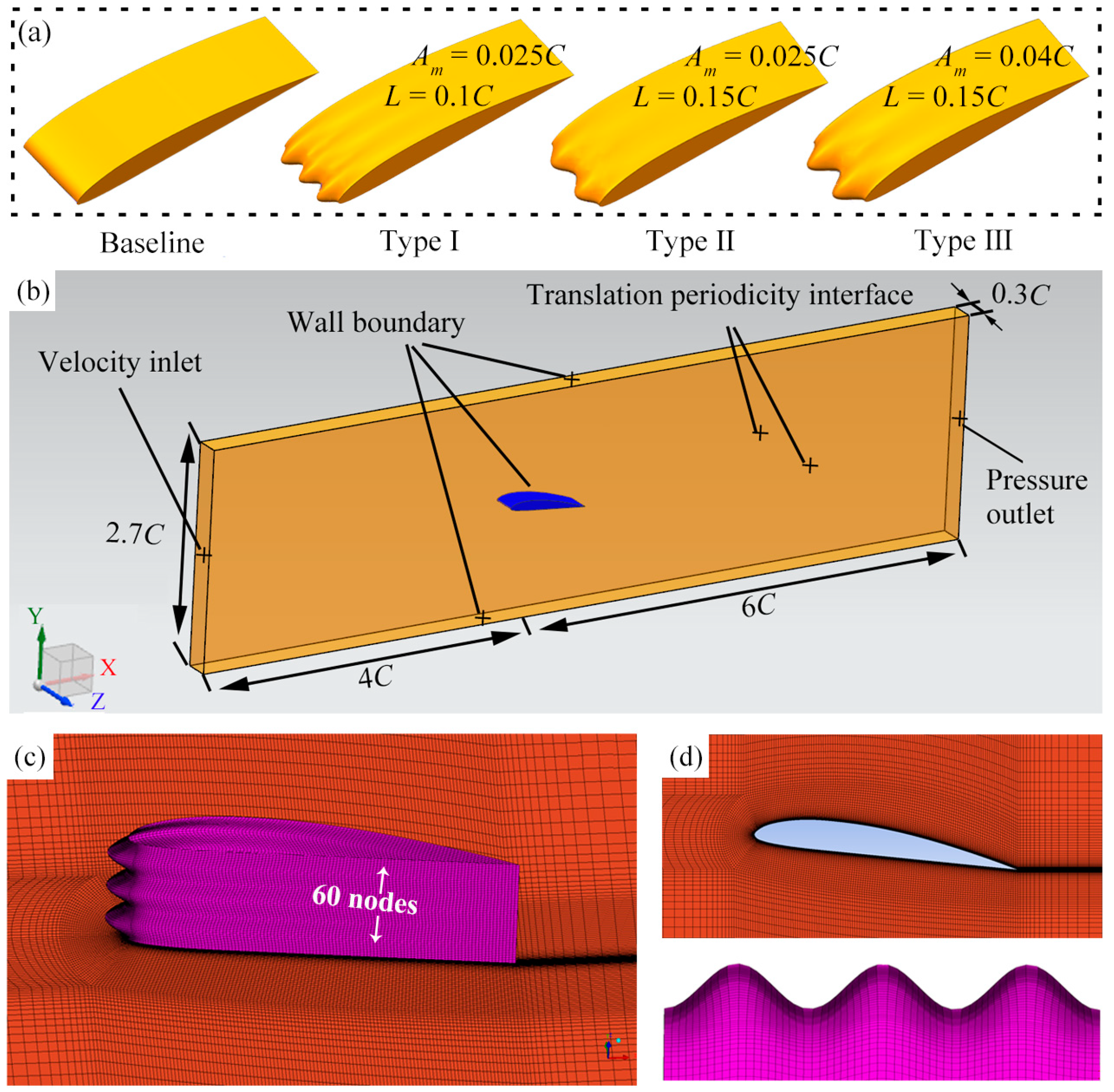
Figure 3.
Grid dependency study for lift and drag coefficients under non-cavitation.

Figure 4.
Numerical results for the four selected hydrofoils at different angles of attack (AOAs): lift coefficient (a), drag coefficient (b), and Cl /Cd ratio (c).
Figure 4.
Numerical results for the four selected hydrofoils at different angles of attack (AOAs): lift coefficient (a), drag coefficient (b), and Cl /Cd ratio (c).
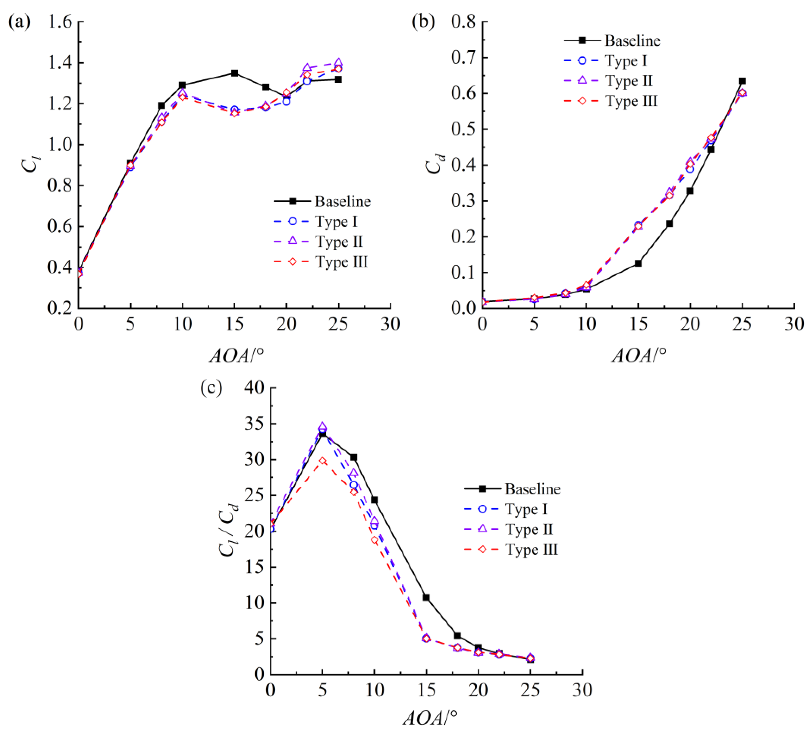
Figure 5.
Velocity magnitude distributions of the mid-spans of the baseline hydrofoil and the peak sections of the modified hydrofoils in the XY plane at AOA = 8°, (a) and AOA = 25° (b).
Figure 5.
Velocity magnitude distributions of the mid-spans of the baseline hydrofoil and the peak sections of the modified hydrofoils in the XY plane at AOA = 8°, (a) and AOA = 25° (b).

Figure 6.
Pressure distribution comparison of the modified hydrofoils’ peak and trough sections with the baseline hydrofoil’s mid-spans for AOA = 8° (a), and AOA = 25° (b).
Figure 6.
Pressure distribution comparison of the modified hydrofoils’ peak and trough sections with the baseline hydrofoil’s mid-spans for AOA = 8° (a), and AOA = 25° (b).
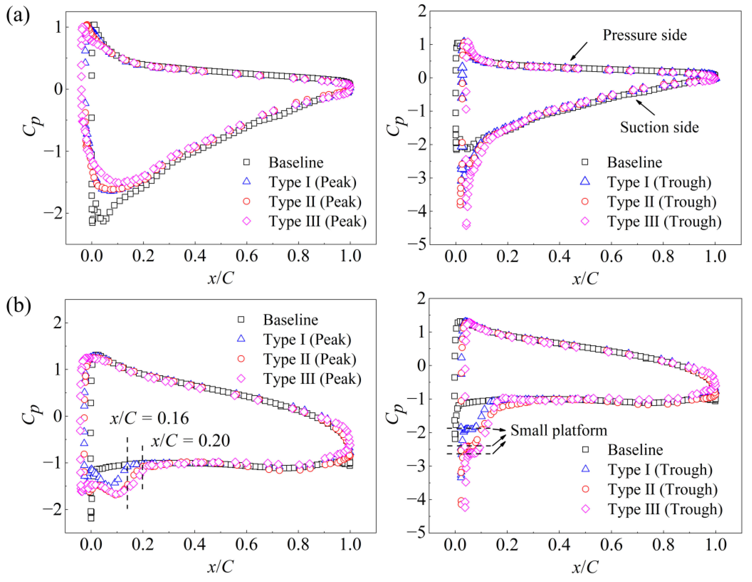
Figure 7.
3D streamlines and streamwise vortices at AOA = 8°: (a) Baseline, (b–d) Type I~III.
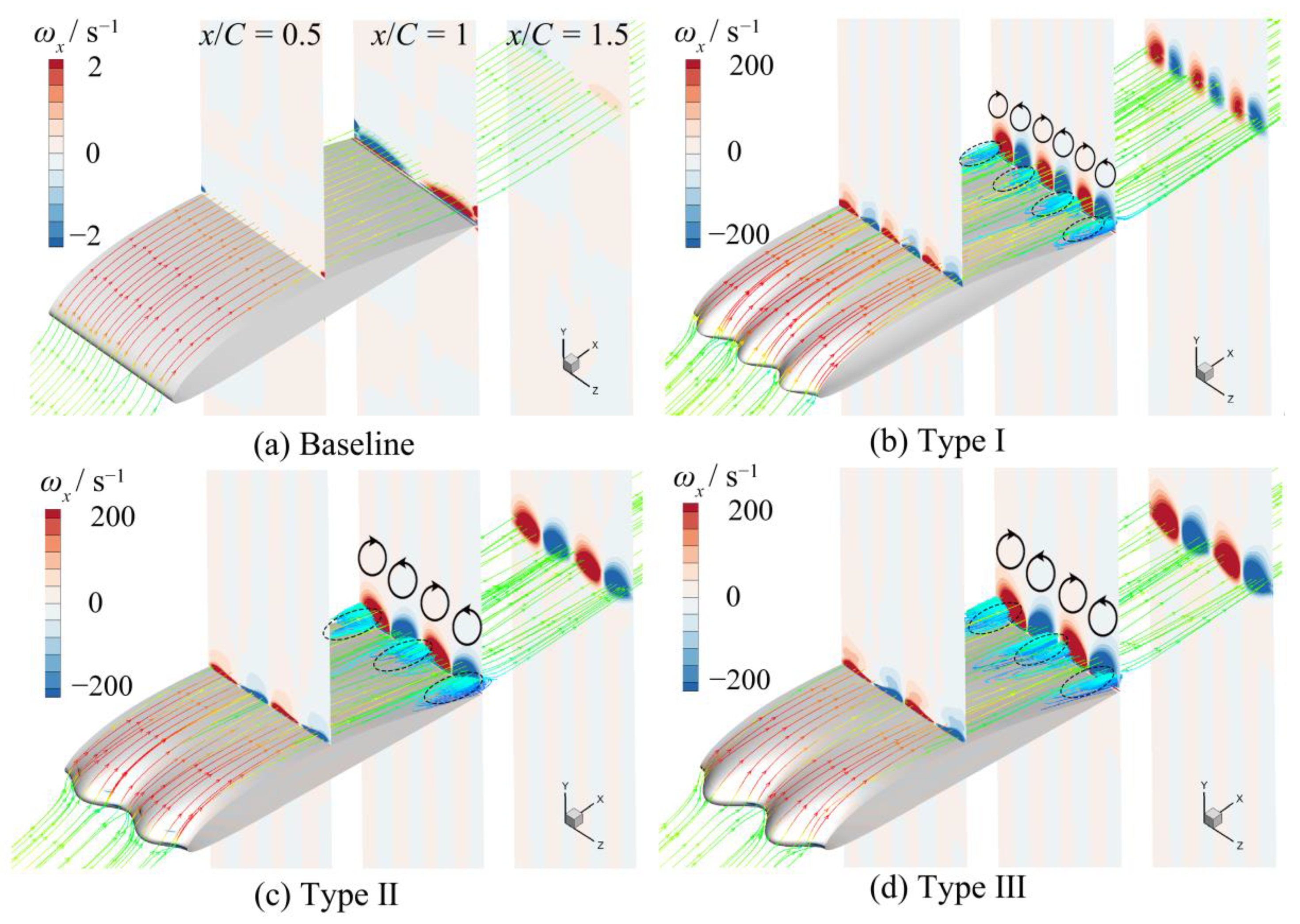
Figure 8.
Numerical dimensionless total vapor volume (V).

Figure 9.
Experimental cavity shape (a), bird’s eye views of the iso-surfaces of αv = 0.1 for the baseline hydrofoil (b), and the modified hydrofoils (c–e).
Figure 9.
Experimental cavity shape (a), bird’s eye views of the iso-surfaces of αv = 0.1 for the baseline hydrofoil (b), and the modified hydrofoils (c–e).

Figure 10.
Pressure gradient and cavity shape contours for the mid-span of the baseline hydrofoil (a), the sections of the peak (b) and the trough (c) of the Type I.
Figure 10.
Pressure gradient and cavity shape contours for the mid-span of the baseline hydrofoil (a), the sections of the peak (b) and the trough (c) of the Type I.
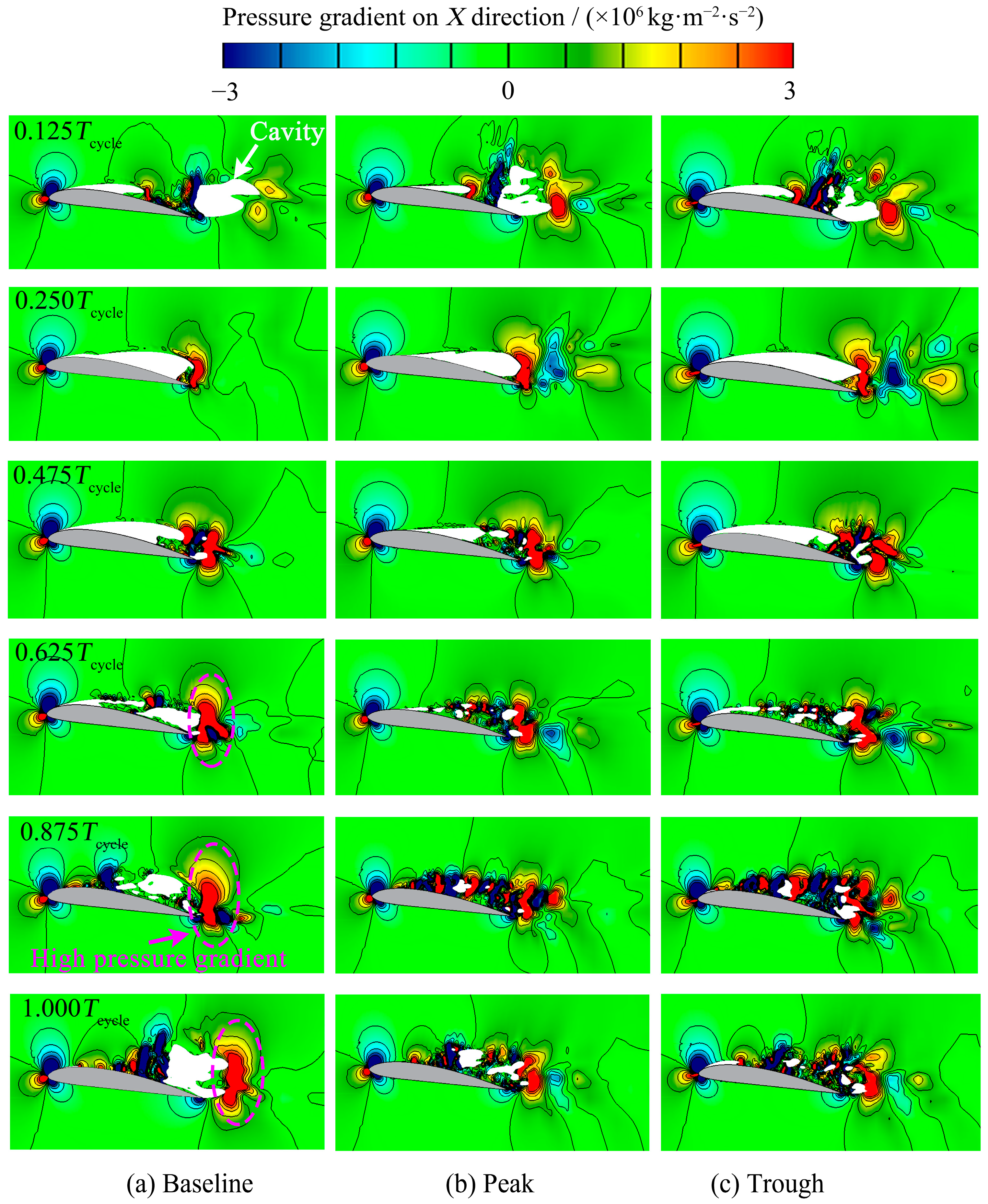
Figure 11.
Flow structures visualized by iso-surfaces with constant value Q = 2 × 10⁴ s−2 (colored by velocity): (a) baseline (b) Type I.
Figure 11.
Flow structures visualized by iso-surfaces with constant value Q = 2 × 10⁴ s−2 (colored by velocity): (a) baseline (b) Type I.
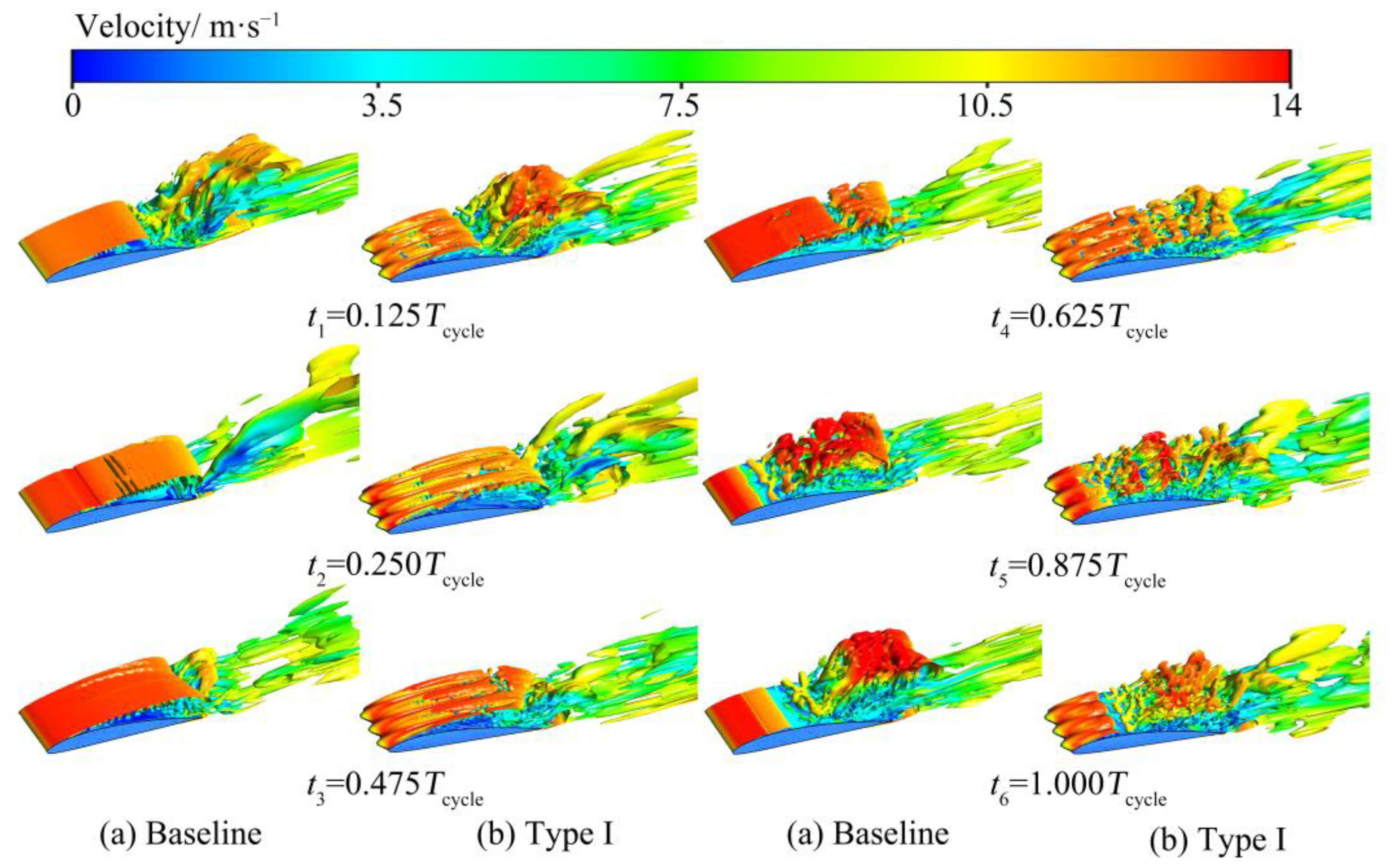
Figure 12.
Iso-surface of ωx = 200 (red) and ωx = −200 (blue) under two conditions.
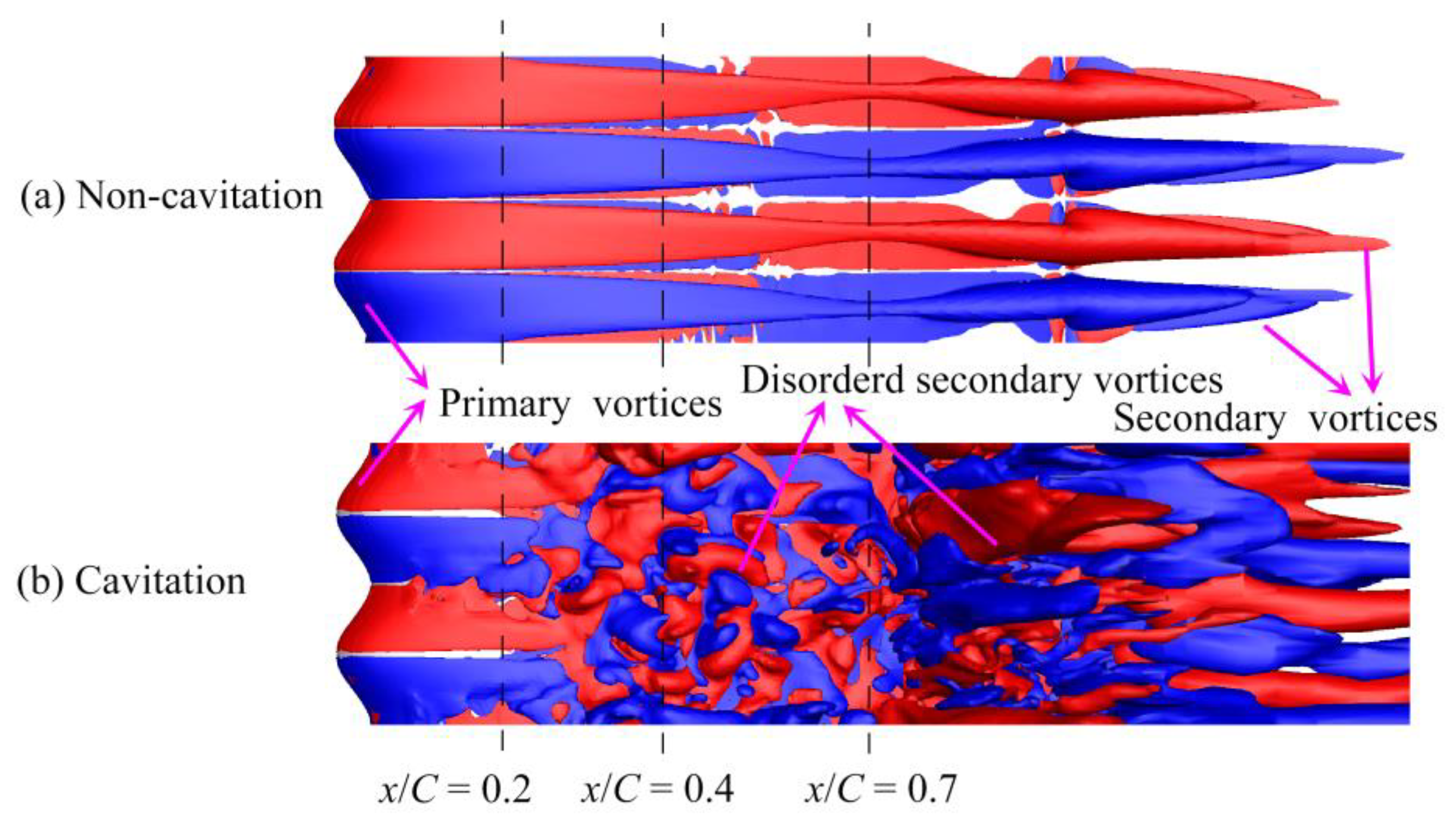
Figure 13.
Predicted vapor volume fraction, vortex stretching term, vortex dilatation term and baroclinic torque term of the modified hydrofoil at different YZ planes.
Figure 13.
Predicted vapor volume fraction, vortex stretching term, vortex dilatation term and baroclinic torque term of the modified hydrofoil at different YZ planes.

Figure 14.
One-dimensional analytical model of pressure fluctuations induced by cavitation.

Figure 15.
One-dimensional analysis results: (a) comparison of the flow rate difference and the first derivative of the V, (b) comparison of the calculated lift coefficient and the second derivative of the V, (c) pressure fluctuations in the unsteady Bernoulli equation, and (d) comparison of the numerical pressure fluctuations and the one-dimensional model.

Table 1.
Numerical uncertainty evaluation based on the GCI indexes.
| Variables | Baseline | Type I | Type II | Type III | |||||
|---|---|---|---|---|---|---|---|---|---|
| Grid | Elements (million) | Cl | GCI (%) | Cl | GCI (%) | Cl | GCI (%) | Cl | GCI (%) |
| Coarse | 0.479 | 1.215 | CGIfine = 0.044 CGImedium = 2.638 | 1.097 | CGIfine = 0.000 CGImedium = 0.266 | 1.106 | CGIfine = 0.057 CGImedium = 0.787 | 1.097 | CGIfine = 0.000 CGImedium = 0.011 |
| General | 0.958 | 1.201 | 1.099 | 1.123 | 1.111 | ||||
| Medium | 1.915 | 1.191 | 1.112 | 1.131 | 1.108 | ||||
| Fine | 2.874 | 1.190 | 1.112 | 1.130 | 1.108 | ||||
Publisher’s Note: MDPI stays neutral with regard to jurisdictional claims in published maps and institutional affiliations. |
© 2021 by the authors. Licensee MDPI, Basel, Switzerland. This article is an open access article distributed under the terms and conditions of the Creative Commons Attribution (CC BY) license (https://creativecommons.org/licenses/by/4.0/).
Share and Cite
MDPI and ACS Style
Li, J.; Liu, C.; Li, X. Effects of Wavy Leading-Edge Protuberance on Hydrofoil Performance and Its Flow Mechanism. J. Mar. Sci. Eng. 2021, 9, 1138. https://doi.org/10.3390/jmse9101138
AMA Style
Li J, Liu C, Li X. Effects of Wavy Leading-Edge Protuberance on Hydrofoil Performance and Its Flow Mechanism. Journal of Marine Science and Engineering. 2021; 9(10):1138. https://doi.org/10.3390/jmse9101138
Chicago/Turabian StyleLi, Jing, Chunbao Liu, and Xiaoying Li. 2021. "Effects of Wavy Leading-Edge Protuberance on Hydrofoil Performance and Its Flow Mechanism" Journal of Marine Science and Engineering 9, no. 10: 1138. https://doi.org/10.3390/jmse9101138
Note that from the first issue of 2016, this journal uses article numbers instead of page numbers. See further details here.