
Multimodel Ensemble Projections of Wave Climate in the Western North Pacific Using CMIP6 Marine Surface Winds


1
CHESS Lab, Graduate School for International Development and Cooperation (IDEC), Hiroshima University, 1-5-1 Kagamiyama, Higashi-Hiroshima 739-8529, Japan
2
Korea-Indonesia Marine Technology Cooperation Research Center (MTCRC), Jakarta 10340, Indonesia
3
Transdisciplinary Science and Engineering Program, Graduate School of Advanced Science and Engineering, Hiroshima University, 1-5-1 Kagamiyama, Higashi-Hiroshima 739-8529, Japan
*
Author to whom correspondence should be addressed.
J. Mar. Sci. Eng. 2021, 9(8), 835; https://doi.org/10.3390/jmse9080835
Submission received: 11 June 2021
/
Revised: 16 July 2021
/
Accepted: 28 July 2021
/
Published: 31 July 2021
(This article belongs to the Special Issue Numerical Models in Coastal Hazards and Coastal Environment)
Abstract
:For decades, the western North Pacific (WNP) has been commonly indicated as a region with high vulnerability to oceanic and atmospheric hazards. This phenomenon can be observed through general circulation model (GCM) output from the Coupled Model Intercomparison Project (CMIP). The CMIP consists of a collection of ensemble data as well as marine surface winds for the projection of the wave climate. Wave climate projections based on the CMIP dataset are necessary for ocean studies, marine forecasts, and coastal development over the WNP region. Numerous studies with earlier phases of CMIP are abundant, but studies using CMIP6 as the recent dataset for wave projection is still limited. Thus, in this study, wave climate projections with WAVEWATCH III are conducted to investigate how wave characteristics in the WNP will have changed in 2050 and 2100 compared to those in 2000 with atmospheric forcings from CMIP6 marine surface winds. The wave model runs with a 0.5° × 0.5° spatial resolution in spherical coordinates and a 10-min time step. A total of eight GCMs from the CMIP6 dataset are used for the marine surface winds modelled over 3 h for 2050 and 2100. The simulated average wave characteristics for 2000 are validated with the ERA5 Reanalysis wave data showing good consistency. The wave characteristics in 2050 and 2100 show that significant decreases in wave height, a clockwise shift in wave direction, and the mean wave period becomes shorter relative to those in 2000.
1. Introduction
Knowledge of wave characteristics is of great importance for marine activities, coastal environments, weather forecasts, and climate change. For instance, significant wave height (Hs), mean wave direction (θ), and mean wave period (Tmn) are commonly used for yachting, fishing, shipping, tourism, and other leisure activities [1]. A wide range of factors, including swell height, fetch, and wavelength, also influence the quality of surfing [2]. Optimal marine transportation and navigation depends on wind wave estimation and simulation [3]. Statistical wave information has become useful in ocean engineering, e.g., for the operation of offshore oil and gas platforms [4] and for the conversion of wave energy to contribute to demands for electricity [5].
Approximately 10% of the global population lives within 20 km of the coastline, and much of this area is lower than 20 m above sea level [6]. Sedimentation and erosion processes due to incoming waves likely affect shore environments and beach morphologies. Shoreline positions are sensitive to directional changes in the waves [7]. Storm surges resulting from high waves and atmospheric pressure [8] can destroy numerous properties and have economic impacts on coastal life, and recovery can take decades [9]. Therefore, comprehensive studies of wind wave characteristics have become crucial for public safety and to minimize the impacts of disasters.
At the global scale, waves play a major role in climate change since oceanic and atmospheric circulation are inseparable. Inversely, climate change also plays a major role in waves. However, how climate change impacts waves, how they have changed over the last century, and how they will change in the future is questionable. Furthermore, if the waves do change in the future, scientific questions arise as to how much these future changes can be predicted and with which level of confidence. Whether the changes are due to the natural variability of the climate or are due to anthropogenic effects must also be investigated. Moreover, the ocean is capable of absorbing or releasing CO2 through wave breaking and white capping [10]. The ocean has its own capacity to absorb emitted gases, but the time that it reaches this peak remains unknown. These findings highlight the importance of studying future wave changes and wave climate projections and its use in a wide range of applications.
Wave climate study demands high-quality wind data with fine temporal and spatial resolutions [11]. Reanalysis datasets and remote sensing products are commonly utilized for past and present data analysis, while the Coupled Model Intercomparison Project (CMIP) dataset is available for modelling historical and future conditions. Reanalysis has the advantages of global coverage and long-term time series data. Historical data from CMIP have been validated by in situ measurements with strong confidence, as shown in many studies [12,13,14]. Numerous model ensembles and future scenarios exist to minimize the uncertainty of projections since there is no future record for reference. CMIP has been used to address environmental and social issues for the upcoming decades [15], including for projections of wave climate [16,17,18,19,20].
Future changes in the multimodel averaged Hs in summer and winter have been projected by applying surface forcing from the CMIP3 dataset and data derived from five independent studies [16]. Global wave modelling was conducted for two time slice experiments with 1979–2009 as the present climate period and 2070–2100 as the future climate period. The projection results show a decrease in Hs over a large area (25.8% of the global ocean) and consistent increases in smaller areas (7.1% of the global ocean). The western North Pacific (WNP) region faces decreasing mean Hs at the end of the century in the projection. This study focuses on wave characteristics instead of extreme waves. Other studies forecast a decrease in the mean and maximum Hs in the South Pacific region in 2100, mainly due to a decrease in the frequency of large tropical cyclones, particularly in boreal winter, while the resulting Hs in the Northern Hemisphere from wave modelling varies with different external forcings from the CMIP3 GCMs [17]. Wave height reduction generally has a linear relationship with projected wind changes in CMIP3 [21]. However, the low temporal and spatial resolutions of surface winds from CMIP3 have limited applications for wind wave studies in shallow coastal environments with complex geometries.
CMIP5 climate models, which have higher spatial resolutions than those from CMIP3, have been applied to observe annual/seasonal extreme wave height changes [18]. Statistical projections of wave characteristics over 6 h were derived from surface winds over 6 h from a number of CMIP GCMs. Significant increases in ocean wave heights were found in the eastern tropical Pacific and at high latitudes of the Southern Hemisphere, and a similar result was found in CMIP3. However, the Hs projection based on CMIP5 input shows more extensive increases than that based on CMIP3 input [18].
CMIP5 has also been used to analyse the implications of global climate change on a regional-scale stormwave climate [19]. Monthly and seasonal changes in the storm wave climate were observed using surface forcing from one GCM in CMIP5 with different future sea surface temperature (SST) conditions. Statistically significant changes in storminess are unlikely to occur in the seas near the United Kingdom. However, an analysis of wave climate changes in the WNP region shows that tropical cyclones, which are sensitive to SST, change their behaviour and influence summertime wave height [20].
The WNP is renowned for its maritime activity, particularly in shipping and transportation [22]. On the other hand, many casualties have occurred in the WNP from typhoons and extreme winds since this region is prone to variability and changes in the wind wave climate [23]. In recent years, although the frequency of oceanic and atmospheric hazards in this region has decreased, the intensity of these hazards has slightly increased or has likely remained the same [24,25]. Advanced information, particularly prospective information on marine surface wind and waves in the WNP, is desirable for long-term weather and extreme event prediction.
Therefore, the objectives of this study are to project the wave characteristics in the WNP in 2050 and 2100. The changes in wave characteristics from the present wave climate to medium-term and long-term scenarios are also assessed. The improved climate dataset, the CMIP6 [26], was composed to answer the remaining issues in the Intergovernmental Panel on Climate Change (IPCC) Fifth Assessment Report (AR5) [27]. As a consequence, our study focuses on projecting wave characteristics in the WNP by implementing marine surface winds from the CMIP6 multi-model ensemble. We use data modelled over 3 h in a dynamic approach by considering extreme winds and typhoons that change drastically in a short time. The ERA5 [28] reanalysis dataset is used as a reference, although considerable deviations from observations still appear. Finally, we discuss the changes in wave characteristics in the context of previous studies.
2. Materials and Method
2.1. Datasets
As described, marine surface winds were retrieved from CMIP6 for wind wave modelling. The finest temporal wind dataset in CMIP, a dataset modelled over 3 h, was used to stimulated wave propagation in the wave model. The resolution of the CMIP spatial grid varies between ~1° and 2.5°. Historical data were retrieved for 2000, while 2050 and 2100 were targeted as the medium-term and long-term future scenarios, respectively. The Atmospheric Model Intercomparison Project (AMIP) in the CMIP includes historical data combined with SST and sea ice concentration in the model experiment [29,30]. The model ensembles used for surface wind forcing in wave modelling are shown in Table 1. Each GCM in the CMIP6 has a different number of ensembles. Each ensemble is distinguished by a variant label, which is indicated with the <r>, <i>, and <p> indices. The label defines the realization number, the initialization method indicator, and the perturbed physics that are explained in the CMIP6 model output requirements [31]. However, the newest CMIP6 put an additional variant called the forcing index or <f> at the end of its variant label.
The shared socioeconomic pathway (SSP) scenarios SSP2-4.5 and SSP5-8.5 in CMIP6 are commonly inspected for middle and extreme cases, respectively, based on additional radiation and mitigation-adaptation challenges in the future. Even though radiation continues to increase until the end of the 21st century, the global emissions decrease in the SSP2-4.5 scenario, while in SSP5-8.5, they only slightly decrease from their peak [32]. All ensembles can be accessed at the Earth System Grid Federation (ESGF) website (https://esgf-node.llnl.gov/search/cmip6/, accessed on 16 July 2021).
The ERA5 hourly dataset with a 0.5° × 0.5° grid resolution for 2000 was retrieved as the reference. The mean wave direction, mean wave period, and mean significant height of the combined wind waves and swell were collected at every hour of each day for wave validation (https://cds.climate.copernicus.eu/cdsapp#!/dataset/reanalysis-era5-single-levels, accessed on 16 July 2021).
Wave propagation from the source is not only dependent on its force but is also affected by bathymetry, particularly in shallow water. The General Bathymetric Chart of the Oceans 2019 (GEBCO_2019) bathymetry, as the latest global bathymetric product with a 15 arc-second grid, was retrieved and used in the wave modelling [33,34]. Global self-consistent hierarchical high-resolution geography (GSHHG) data were applied in the model as the displayed boundaries [35]. The GSHHG data can be retrieved from https://www.soest.hawaii.edu/pwessel/gshhg/ (accessed on 16 July 2021). The bathymetry and shoreline for the wave modelling domain are plotted in Figure 1.
2.2. Wave Modelling
Wave characteristics were simulated by WAVEWATCH III v5.16 (WWIII) based on the energy balance equation and the Eulerian approach [36]. It is widely used in theoretical studies and practical applications for wind–wave processes and operational forecasts at both the global and regional scales. The balance equation is described by , where is the total derivative, is the action density spectrum, and S represents the net source and sink terms for the spectrum . , , and are the wavenumber, direction, and relative frequency, respectively. The balance equation for the action density used in WWIII takes the following conservative form
where , , and are the wavenumber vector, the mean water depth, and the depth-and time-averaged current velocity, respectively. is given by , the group velocity, and . is a coordinate in the direction of , and is a coordinate perpendicular to . The left-hand side of Equation (1) represents the evolution of the wave density spectrum, , which considers linear wave propagation as a result of physical processes on the right-hand side. The physical processes are mainly the wind input from the atmosphere, ; the nonlinear wave–wave interactions within the spectrum, ; the wave energy dissipation due to whitecapping, ; and the wave decay due to bottom friction in shallow water, . For extremely shallow water, the wave energy dissipation due to depth-induced breaking, , is introduced from WWIII version 3.14 [37,38].
2.3. Wave Model Setups
Wind–wave simulation was conducted for the WNP, defined as 110° E–170° E and 10° N–60° N (Figure 1). The domain was enlarged by 5° surrounding the WNP region as a buffer zone to avoid boundary issues since there was no external boundary input imposed, for example, from a global wind wave model. The computational domain consisted of a total of 141 × 121 grids with a 0.5° spatial resolution. Bathymetry data and CMIP6 marine surface winds were also interpolated onto the half-degree resolution grid space. The spectral grid was composed of 24 directions and 25 frequencies exponentially spaced from 0.04118 Hz with an increment of 10%. The maximum global time step, the maximum Courant–Friedrichs–Lewy (CFL) time steps for x-y and k-theta, and the minimum source term in WWIII were determined to be 1800, 950, 900, and 600 s, respectively.
Each scenario used an identical parameter setting that could be tuned by the user. Nonlinear wave interactions were modelled through the discrete interaction approximation (DIA), which was originally developed for spectra [39,40]. The linear input of Cavaleri and Malanotte-Rizzli [41] allows the consistent spin-up of a model and improves the initial wave growth behaviour. The parameterization of Tolman [42], which was adjusted by Ardhuin et al. [43], was used () for the bottom friction. The bottom friction was adjusted from the Shoaling Waves Experiment (SHOWEX) measurements on the North Carolina continental shelf. Depth-induced breaking algorithms used the approach of Battjes and Janssen [44], which assumes that all waves exceeding a threshold height will break. A Miche-type criterion [40] was used to define the maximum wave height (). The shoreline reflection setting was activated in the model. Additional source terms were switched off, such as bottom scattering , damping and scattering by sea ice , and user-defined source terms .
The model was compiled with the ST4 source term package, which includes flux computation (FLX0, STAB0) [45]. ST4 was chosen after sensitivity tests by comparing the resulting wave characteristics with other source terms. The propagation used a third-order propagation scheme (UQ) that is accurate in both space and time. Additionally, Tolman’s averaging technique (PR3) was used for spatial averaging [46]. The parameter settings that were used were similar to the global and East Pacific model produced by the National Oceanic and Atmospheric Administration (NOAA) (https://polar.ncep.noaa.gov/waves/implementations.php, accessed on 16 July 2021), except for that the reflection term was switched on. The summary of model setups is presented in Table 2.
The results of wave characteristics modelled over 3 h were produced from the WWIII modelling, and each wave characteristic from each ensemble was averaged and compared to each scenario in a spatial map. For validation, the resulting wave characteristics were compared to the ERA5 wave output. Finally, historical (2000) and future (2050 and 2100) multimodel mean significant wave heights (mean Hs), maximum significant wave heights (extreme Hs), mean wave directions, and mean wave periods could be obtained.
3. Results
3.1. Wave Validation
The validation of the WWIII model was accomplished with 3-h surface wind model from 8 ensembles of CMIP6 for 2000 (Figure 2). The wave outputs were then compared with the reference wave characteristics retrieved from ERA5. The model and reference show similar patterns for mean Hs. Higher Hs is found off eastern Japan, with an average of 3 m, than in other regions. The other regions have mean Hs of 2–2.5 m, and smaller Hs are discovered near coastal areas. The model Hs are approximately 0.1–0.4 m higher than the reference Hs in some regions, such as the northern part of the Philippines, the Japan/East Sea, and the Sea of Okhotsk (50°–60° N and 140°–150° E). In regions closer to the centre of the Pacific and in coastal areas, the model Hs are 0.1–0.4 m lower than those of the reference.
Generally, wave directions have small differences between the model and the reference. Waves from the simulation propagate in a more clockwise direction than the waves in the reference, particularly in the eastern part of the domain. Positive differences indicate that the wave direction in the model is shifted more in the clockwise direction, while negative values indicate the opposite. The angle differences are not wide, approximately 10°–50° at each grid. For an easier comparison, black vector arrows were placed on the graph. The reference shows a mean wave period of 8 s in the WNP, but some parts of the domain have a wave period of 5 s, particularly in the Japan/East Sea region. Obstacles and different seabed features can influence the wave period. The model produces shorter periods, with a range of 0.5–2 s, than the reference. Considering the validation results, the WWIII model settings can be used further to simulate future wave projections.
The wave simulation validation was only performed for 2000. Indeed, a more extended simulation represents the wave pattern with higher confidence. Therefore, the results are also compared to those from the study of Hemer et al. [16]. They show an averaged multimodel annual Hs from 1979–2009, which represents the present climate in the global domain. The region east of Japan has Hs of approximately 3 m, while the rest of the WNP domain has Hs of approximately 2–2.5 m. The average Hs from this study, even though they consist of only a 1-year simulation, are similar to their pattern from 30-year simulation, and the values are not much different, such that the 30-year result shows that the average Hs is approximately 1.5–3 m, whereas the 1-year simulation of this study depicts an average Hs of 1.5–3.25 m. The mean wave period in the WNP is approximately 6–8 s; however, the results of this study produce a shorter wave period of approximately 1–1.5 s depending on the location of the domain. Their results show a clear distinction in the wave direction along 30° N. The results of this study show that waves propagate to the west, the Japan coast, and the northern domain. The main differences between the two studies are the total ensembles that are involved in the simulations. They consider 20 ensembles for Hs and five ensembles for wave direction and period from other studies, including CMIP3.
3.2. Historical and Future Wave Characteristics
The wave characteristic results of the WWIII simulation are shown in Figure 3, Figure 4, Figure 5 and Figure 6. Wave time series were simulated for one-year periods (2000, 2050, and 2100) from 8 ensembles with a 3-h atmospheric dataset. The exact values are shown for the AMIP scenarios in Figure 3, Figure 4, Figure 5 and Figure 6, while the other panels in the figures show the differences between each future scenario and the historical AMIP scenario. For Hs, a positive (negative) value indicates a higher (lower) Hs in the future. For the future wave direction, positive (negative) means that waves will shift more clockwise (counterclockwise). A positive mean wave period indicates a longer wave period in the future, and vice versa. In the medium-term (2050) and the long-term (2100) scenarios, changes are observed, although the values are not significant.
The average Hs in 2000 reached 3.5–4 m in eastern Japan and were between 30° and 50° N and 150° and 170° E (Figure 3). The rest of the region had an average Hs of 1.5–2 m. The white colour indicates regions with small changes in the future compared to the AMIP scenarios. In the medium-term scenario of SSP2-4.5 (Figure 3b), wave heights decrease by approximately 0.1–0.5 m. The largest decreases occur in the area between Taiwan and the Philippines (20° N and 115°–130° E). However, wave heights increase by up to 0.1 m in the Japan/East Sea and the northern domain and by up to 0.2 m in the southeastern domain of the WNP. In 2100 (Figure 3c), the area with decreasing Hs extends farther to the north; moreover, the region with increasing Hs surrounding Japan decreases spatially. Additionally, the area with the largest decreases becomes smaller spatially. The future wave heights remain the same as the historical wave heights in the southeastern domain. The increasing Hs in the Pacific is followed by the higher wind speed output from the CMIP6 [30].
In the medium-term scenario of SSP5-8.5 (Figure 3d), the decrease in Hs has a similar pattern to that in the SSP2-5.4 long-term scenario. A small region with a 0.3 m reduction is discovered at approximately 32° N and 160° E in the SSP5-8.5 medium-term scenario and is larger in the SSP5-8.5 long-term scenario. In the long-term output (Figure 3e), almost the entire WNP faces decreasing Hs. The southeastern region of the WNP study domain encounters a decreasing Hs, which is different than the rest of the scenario. Generally, the mean Hs will decrease in the future, although the value is not substantial.
The waves north of 20° N propagate to the north and northeast, while in the southern domain of the WNP, they propagate to the west (Figure 4a). Waves from the Pacific likely propagate to the Japan coast. For the average direction in medium-term scenarios, in either SSP2-4.5 or SSP5-8.5, waves tend to shift more clockwise by approximately 5°–20°. Only a small part of the WNP has a wave direction that turns more toward the counterclockwise direction, i.e., the northern part of Japan and the region located at 150°–170° E and 15°–25° N. The wave direction changes by −30° or more in the complicated geometric area among the islands of the Philippines in the medium-term projections. However, due to the unreliable grid size between those islands, it is difficult to further analyse this result.
In the long-term projections, average waves still shift clockwise. Significant changes were discovered south of Japan in the SSP2-4.5 scenario (Figure 4c) and in the east of Japan (EJ) subregion for the extreme scenario of SSP5-8.5 (Figure 4e). The rest of the WNP is dominated by changes in wave directions of approximately 5°–15° clockwise. The area close to the central Pacific has wave direction changes of 20°–25°. The wave direction in the small region south of Japan in the SSP2-4.5 medium-term scenario (Figure 4b) shifts 5° more clockwise in the long-term scenario (Figure 4c). A large region with extreme shifts averaging +20° was found east of Japan under the SSP5-8.5 long-term scenario (Figure 4d).
The average wave period in 2000 was approximately 7 s for most regions in the WNP (Figure 5a). However, in the Japan/East Sea and the inner part of the Yellow Sea, the period was lower by approximately 4.5–5.5 s. In the SSP2-4.5 medium-term scenario, the mean wave period decreased by 0.2 s south of Japan and decreased more in the region closer to the Philippines (Figure 5b). Some areas in the northern part of the WNP study domain and to the west of Japan have increases in the wave periods. The region with increases in the wave periods is smaller in 2100 (Figure 5c) than in 2050. In the extreme medium-term scenario (Figure 5d), the areas with a decreasing wave periods of 0.2 s and 0.3 s (shown by light blue colour) are wider than those in the SSP2-4.5 scenario. A different SSP scenario in the same year gives a different mean wave period, whereas the extreme case produces a lower value. In the SSP5-8.5 long-term projection (Figure 5e), the region south of Japan has a mean wave period reduction of 0.3 s. Moreover, a −0.5 s period change is found in the northern part of the WNP study domain.
In the future, the mean wave period decreases by 0.1–0.5 s, although the wave period remains the same or increases in a small region. There is no substantial difference between the medium-term and long-term scenarios, and the only change is in the distribution of the area with a decrease in wave period. The region with a shorter wave period disperses more to the centre of the WNP domain. The region in the southeastern domain has a mean wave period that decreases by 0.5 s in every scenario.
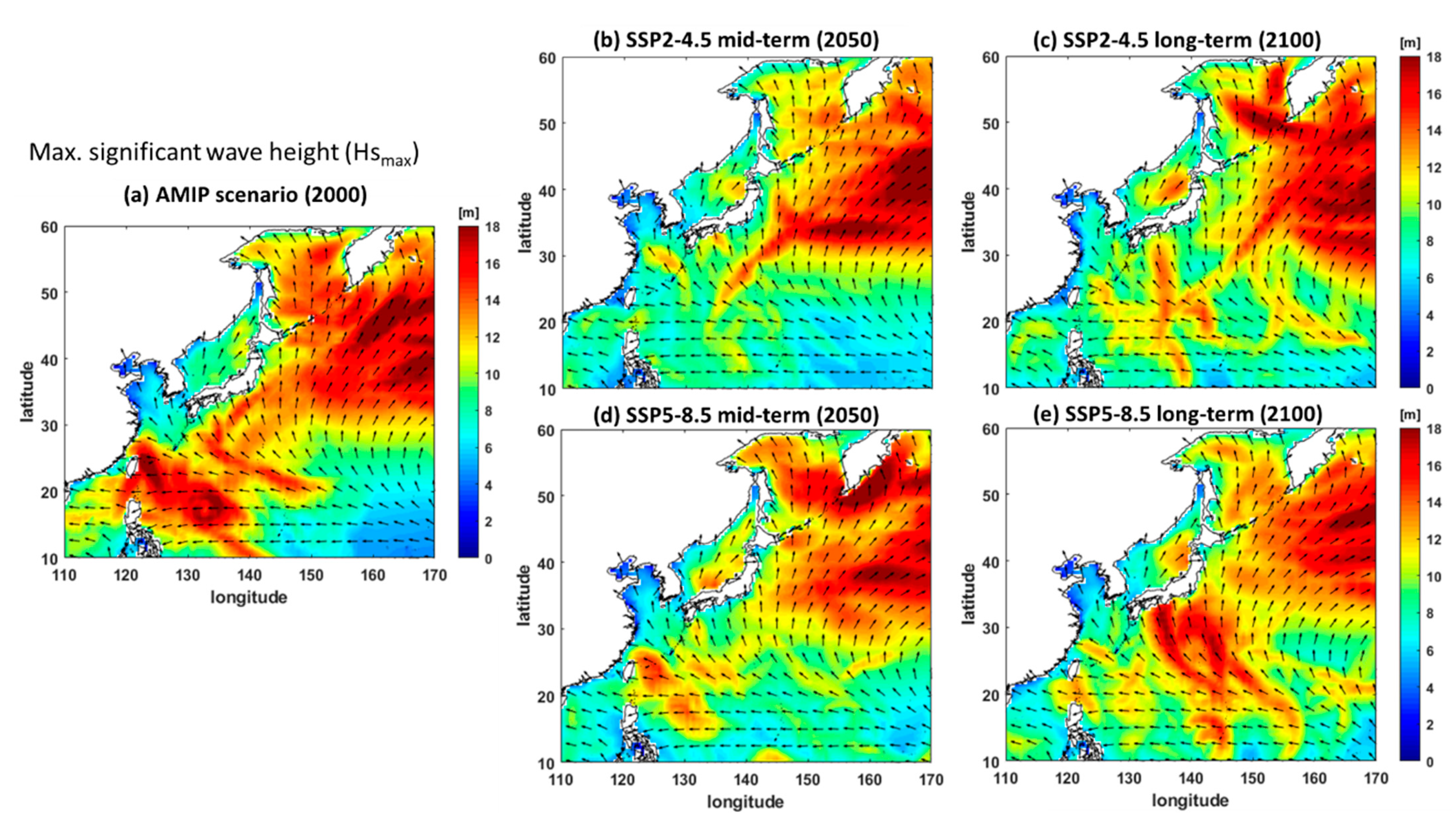
The observed extreme significant wave height was determined by calculating the annual maximum Hs from the WWIII output (Figure 6). The arrows in Figure 6 show the average wave direction since it is not wise to show the maximum or minimum angle at each grid. In 2000, an extreme wave was found in the southern part and in the eastern part of the WNP (Figure 6a). The annual maximum Hs can be 18 m. In each future scenario, the maximum Hs shifts to the northern part of the domain. The red region, which indicates Hs of approximately 14–18 m, is found east of Japan, although the southern part of the WNP still has high Hs.
In the medium-term scenario of SSP2-4.5 (Figure 6b,d), the maximum Hs region still exists in the eastern part of the WNP domain. However, the highest Hs south of Japan is reduced to 8–10 m, although Hs of 14 m is found in this area in the SSP5-8.5 medium-term scenario. There was no difference in the high Hs region east of Japan between the medium-term and long-term scenarios (Figure 6c,e). In the long-term scenario, the wave heights in the eastern part of the WNP seem to decrease by approximately 0.5–1 m. However, there are some extreme Hs that propagate directly to Japan (Figure 6e).
Further, the projected monthly and seasonal wave characteristics for both scenarios in 2050 and 2100 can be found in Supplementary Material.
4. Discussion
The multimodel ensemble averaged Hs in 2050 and 2100 is 0.1–0.5 m lower than that in the historical model. The results around Japan are consistent with Shimura et al. [47]. The projected decreases in Hs have a high degree of confidence since the projected future changes are highly consistent among the ensemble results. Shimura et al. projected a decrease in wave height in the central North Pacific along 30°–40° N. However, the mean Hs in this study increases by approximately 0.2 m in the region close to the centre of the North Pacific. There is a difference in wind input over the WNP region between this study and that of Shimura et al. Undeniably, certain GCMs carry more uncertainties and anomalies for wind datasets. Moreover, particular phenomena such as extreme winds or tropical cyclones cannot be considered with 3- or 6-h surface winds. Therefore, the Hs results in this study close to the central North Pacific are slightly different. Decreasing wave heights correspond to positive changes in the West Pacific (WP) pattern (climate indices) [47].
Wang et al. [18] derived 20 ensembles from CMIP5 to investigate the annual mean and maximum Hs at the global scale. The historical average Hs in the WNP region is around 1.5–3 m. They are validated with ERA40 and ERA-Interim. Although our model produces higher mean Hs (up to 0.5 m higher), the Hs pattern is similar. A higher Hs is located in the east of WNP and continues to decrease close to southwest part of the domain. Wave height in the future in the Northern Hemisphere is likely to decrease, while a significant increase will occur in the tropics (especially the eastern tropical Pacific) and the Southern Hemisphere high latitudes (south of 45°). The wave height changes were primarily driven by the changes in the marine surface wind and the increase in the spatial sea level pressure. Almost in the WNP region (above 25° N), the annual mean Hs will decrease up to 0.2 m in the future; meanwhile, in the southern part of the WNP (10°−25° N), Hs is slightly increasing by approximately 0.06 m. Our future projection shows a similar range of Hs changes, but some areas show noticeable differences, such as the decreasing Hs (up to 0.5 m) in the northern part of the Philippines and the increasing Hs (0.1 m) around Japanese islands. The differences in CMIP marine surface wind, input resolution, and wave model grid might be one of the reasons for this.
High resolution of future wave projection in global coverage was investigated by Timmermans et al. [48], although the atmospheric model was mainly from CAM5, one of the CMIP5 products. The wave model of 1° and 0.25° was compared. The higher resolution showed more variation in the future projection (RCP8.5) around the WNP region. In the results of the 0.25° model, the increasing and decreasing areas were very close and alternated. In contrast, Shimura et al. [20], Wang et al. [18], and this study show more distinctive contours in displaying Hs changes due to the use of a coarser grid.
A global wave climate ensemble were also performed and stored under Coordinated Oean Wave Climate Project (COWCLIP) Phase 2. The COWCLIP comprises 155 ensembles obtained from ten CMIP5 wave climate studies. Morim et al. [49], validated each wave ensemble with satellite measurements (wave heights only) between 1991−2017. It was shown that the ensemble had good correlation with references (correlation above 0.9) with a centred root mean squared under 0.5 m and a normalized standard deviation of approximately 1 m. The WWIII main model setting that was used was not different from the configuration of this study. From their results, it is known that the CMIP ensemble is reliable enough to calculate historical scenarios.
It is expected that different future scenarios would lead to the appearance of different wave characteristics. However, it was found that the marine surface wind output from CMIP have not been much different over the decades [30]. The results of the wave characteristic analyses from the SSP2-4.5 and SSP5-8.5 scenarios are not significantly distinct. This result is very different from the temperature or emission projections, which can clearly distinguish between each future scenario [50].
Even though the wave height can decrease, the mean sea level continues to increase year by year. The mean rate of global average sea level rise was 1.5 to 1.9 mm/year between 1901 and 2010, 1.7 to 2.3 mm/year between 1971 and 2010, and 2.8 to 3.6 mm/year between 1993 and 2010 [51]. For example, long term wave scenarios with and without sea level rise were investigated locally by Chini et al. [52]. The effect of sea level rise leads to an increase in inshore wave height in shallow waters. Due to sea level rise, a significant wave height with a 100-year return period without sea level rise becomes more frequent. Additionally, shorelines that are currently protected by sandbanks are more likely to face waves with a higher proportional increase in height. Thus, the analysis should consider sea level rise in future scenarios.
The multimodel ensemble projection of wave climate considers CMIP6 marine surface wind as the only primary forcing. However, other factors such as sea level variation, tides, river run-off, ice, and ocean currents can affect waves and wave climate. Additionally, other reanalysis data should be considered as references. Longer-term simulations can represent additional aspects of the wave climate. Hemer et al. [16] simulated over 30 years, while this study considered only a one-year simulation. Although the mean wave characteristics are still similar when both are compared, a longer simulation with a higher spatial resolution will provide other insights into wave characteristics.
The uncertainty comes from ensemble forcing, the quantity of GCMs, downscaling methods, and model physics parameterizations [16]. Increasing the forcing of the simulation might solve this matter, but the question is how significant other forcings are in wave behaviour in the WNP region. Increasing the number of GCMs can sometimes increase uncertainty. Thus, careful investigation of the available GCMs and their output is needed to reduce the uncertainty. The resolution in wave climate simulation is still coarse to reflect the shallow coastal zone and environment, although 0.5° is sufficient for regional wave modelling. Previous studies and reanalysis implemented various spatial resolutions, for example, 0.5° in ERA5, 0.75° in ERA-Interim, 1° in Wang et al. [18], 1.5° in Hemer et al. [16], and 2.5° in Liu et al. [53] for global and regional applications. Obviously, observing a local or specific events (typhoons, storm surges, etc.) needs a smaller grid size. Therefore, a nesting method or multimodel downscaling is necessary to further consider a specific shallow water and coastal environment. The output produced by this study, i.e., waves and marine surface winds within the study domain, can be the input for finer model downscaling and be used for the estimation of wave power generation.
In this study, it is predicted that the mean significant wave height will decrease by 0.1 to 0.5 m, the wave direction will rotate clockwise by 5 to 25 degrees, and the wave periods will decrease by 0.1 to 0.5 s. It should be noted that the predicted changes are smaller than the typical errors in the validation, so they should be taken as indicating the expected wave and magnitude of change, but the models do not necessarily give absolute predictions of this accuracy.
5. Conclusions
Wave characteristics will change in the future. Based on the future scenarios of SSP2-4.5 and SSP5-8.5, the decrease in multimodel averaged Hs may reach 0.5 m. The mean wave direction is projected to shift more clockwise by up to 25°, while the mean wave period is projected to decrease by 0.1–0.5 s. The annual maximum Hs may reach 18 m or more; however, the region with largest increases in Hs will shift to the northeast. Several prior studies have projected future wave characteristics involving the CMIP 3 and 5 datasets [16,17,18,19,20,47]. This study illustrated analogous results in wave climate projections such as wave heights, wave periods, and wave directions in the WNP using CMIP6 marine surface winds as the latest climate dataset. Moreover, it can be a benchmark for further research to obtain a better result in analysing future wave climate in the same study region.
Comprehensive research is necessary to observe the wave climate over the WNP region. A global domain is worth investigating to see the global characteristics of the wave climate and their relationship with atmospheric climate indices. The specific area needs to be examined through a nesting method with initial and boundary inputs from global and regional model outputs. The coarse resolution used in global simulation hardly distinguishes some areas, i.e., islands and coastal regions, due to the size of the grid in the model. One method to overcome the resolution issue of global GCMs is the application of dynamic downscaling [54]. It will be worthwhile to investigate in more detail to determine the impact on the coastal environment and the coastal risk for sustainable coastal zone management and development.
In this study, a qualitative comparison between the AMIP scenario for 2000 and the future scenarios of 2050 and 2100 was made. Thus, the statistical assessment of model performance and significance could not be performed and remain as topics for further study. Additionally, in future work, long-term simulations are needed to investigate the annual, interannual, and decadal variability in wave characteristics due to climate change. Other limitations of this study such as the boundary condition from global wave climate modelling and the temporal resolution of atmospheric forcing (marine surface winds) over 3 h, and their effects should be investigated and improved in future work. In particular, extreme waves induced by tropical cyclones and extratropical cyclones cannot be simulated by 3-h global GCMs surface wind model.
Supplementary Materials
The following are available online at https://www.mdpi.com/article/10.3390/jmse9080835/s1, Figure S1: Mean significant wave height (Hs in m) results for AMIP scenario and the differences between each future scenario and the AMIP scenario for January-April. Positive (negative) value indicates increasing (decreasing) wave height in the future relative to AMIP values. Figure S2: The same as Figure S1, but for May-August. Figure S3: The same as Figure S1, but for September-December. Figure S4: Mean wave direction ( in degree) results for AMIP scenario and the differences between each future scenario and the AMIP scenario for January-April. Positive (negative) value indicates wave direction shifting clockwise (counter clockwise) in the future relative to AMIP values. Figure S5: The same as Figure S4, but for May-August. Figure S6: The same as Figure S4, but for September-December. Figure S7: Mean wave period ( in second) results for AMIP scenario and the differences between each future scenario and the AMIP scenario for January-April. Positive (negative) value indicates increasing (decreasing) wave period in the future relative to AMIP values. Figure S8: The same as Figure S7, but for May-August. Figure S9: The same as Figure S7, but for September-December. Figure S10: Mean significant wave height (Hs in m) results for AMIP scenario and the differences between each future scenario and the AMIP scenario for each season. Positive (negative) value indicates increasing (decreasing) wave height in the future relative to AMIP values. Figure S11: Mean wave direction ( in degree) results for AMIP scenario and the differences between each future scenario and the AMIP scenario for each season. Positive (negative) value indicates wave direction shifting clockwise (counter clockwise) in the future relative to AMIP values. Figure S12: Mean wave period ( in second) results for AMIP scenario and the differences between each future scenarios and the AMIP scenario for each season. Positive (negative) value indicates increasing (decreasing) wave period in the future relative to AMIP values.
Author Contributions
Conceptualization, M.R.B.; formal analysis, M.R.B. and H.S.L.; writing—original draft preparation, M.R.B. and H.S.L.; writing—review and editing, M.R.B. and H.S.L.; supervision, H.S.L. All authors have read and agreed to the published version of the manuscript.
Funding
This research was partly supported by the Grant-in-Aid for Scientific Research (17K06577) from JSPS, Japan.
Institutional Review Board Statement
Not applicable.
Informed Consent Statement
Not applicable.
Data Availability Statement
MDPI Research Data Policies.
Acknowledgments
The first author is supported by the JICA Innovative Asia Program.
Conflicts of Interest
The authors declare no conflict of interest.
References
- Caldwell, P.C.; Aucan, J.P. An Empirical Method for Estimating Surf Heights from Deepwater Significant Wave Heights and Peak Periods in Coastal Zones with Narrow Shelves, Steep Bottom Slopes, and High Refraction. J. Coast. Res. 2007, 23, 1237–1244. [Google Scholar] [CrossRef] [Green Version]
- Buckley, R.C. Surf Tourism and Sustainable Development in Indo-Pacific Islands. I. The Industry and the Islands. J. Sustain. Tour. 2002, 10, 405–424. [Google Scholar] [CrossRef] [Green Version]
- Chen, C.; Shiotani, S.; Sasa, K. Numerical Ship Navigation Based on Weather and Ocean Simulation. Ocean. Eng. 2013, 69, 44–53. [Google Scholar] [CrossRef] [Green Version]
- Niedzwecki, J.M.; Huston, J.R. Wave Interaction with Tension Leg Platforms. Ocean. Eng. 1992, 19, 21–37. [Google Scholar] [CrossRef]
- Drew, B.; Plummer, A.R.; Sahinkaya, M.N. A Review of Wave Energy Converter Technology. Proc. Inst. Mech. Eng. Part. A J. Power Energy 2016, 223, 887–902. [Google Scholar] [CrossRef] [Green Version]
- Kummu, M.; de Moel, H.; Salvucci, G.; Viviroli, D.; Ward, P.J.; Varis, O. Over the Hills and Further Away from Coast: Global Geospatial Patterns of Human and Environment over the 20th–21st Centuries. Environ. Res. Lett. 2016, 11, 034010. [Google Scholar] [CrossRef]
- Coelho, C.; Silva, R.; Veloso-Gomes, F.; Taveira-Pinto, F. Potential Effects of Climate Change on Northwest Portuguese Coastal Zones. ICES J. Mar. Sci. 2009, 66, 1497–1507. [Google Scholar] [CrossRef] [Green Version]
- Flather, R.A. Storm Surges. In Encyclopedia of Ocean Sciences; Steele, J.H., Ed.; Elsevier: Woods Hole, MA, USA, 2001; Volume 5, pp. 530–540. [Google Scholar] [CrossRef]
- Lotze, H.K.; Coll, M.; Magera, A.M.; Ward-Paige, C.; Airoldi, L. Recovery of Marine Animal Populations and Ecosystems. Trends Ecol. Evol. 2011, 26, 595–605. [Google Scholar] [CrossRef] [Green Version]
- Zhao, D.; Toba, Y.; Suzuki, Y.; Komori, S. Effect of Wind Waves on Air’sea Gas Exchange: Proposal of an Overall CO2 Transfer Velocity Formula as a Function of Breaking-Wave Parameter Effect of Wind Waves on Air-Sea Gas Exchange: Proposal of an Overall CO2 Transfer Velocity Formula as a Function of Breaking-Wave Parameter. Tellus B Chem. Phys. Meteorol. 2003, 55, 478–487. [Google Scholar] [CrossRef] [Green Version]
- Caires, S.; Sterl, A.; Bidlot, J.-R.; Graham, N.; Swail, V. Intercomparison of Different Wind-Wave Reanalyses. J. Clim. 2004, 17, 1893–1913. [Google Scholar] [CrossRef]
- Mori, N.; Shimura, T.; Kamahori, H.; Chawla, A. Historical Wave Climate Hindcasts Based on JRA-55. In Proceedings of the Coastal Dynamics, Helsingør, Denmark, 12–16 June 2017; pp. 117–124. [Google Scholar]
- Chawla, A.; Spindler, D.M.; Tolman, H.L. Validation of a Thirty Year Wave Hindcast Using the Climate Forecast System Reanalysis Winds. Ocean. Model. 2013, 70, 189–206. [Google Scholar] [CrossRef]
- Wen, C.; Kumar, A.; Xue, Y. Uncertainties in Reanalysis Surface Wind Stress and Their Relationship with Observing Systems. Clim. Dyn. 2019, 52, 3061–3078. [Google Scholar] [CrossRef]
- Schweikert, A.; Espinet, X.; Chinowsky, P. The Triple Bottom Line: Bringing a Sustainability Framework to Prioritize Climate Change Investments for Infrastructure Planning. Sustain. Sci. 2018, 13, 377–391. [Google Scholar] [CrossRef]
- Hemer, M.A.; Fan, Y.; Mori, N.; Semedo, A.; Wang, X.L. Projected Changes in Wave Climate from a Multi-Model Ensemble. Nat. Clim. Chang. 2013, 3, 471–476. [Google Scholar] [CrossRef]
- Fan, Y.; Held, I.M.; Lin, S.; Wang, X.L. Ocean Warming Effect on Surface Gravity Wave Climate Change for the End of the Twenty-First Century. J. Clim. 2013, 26, 6046–6066. [Google Scholar] [CrossRef]
- Wang, X.L.; Feng, Y.; Swail, V.R. Changes in Global Ocean Wave Heights as Projected Using Multimodel CMIP5 Simulations. Geophys. Res. Lett. 2014, 41, 1026–1034. [Google Scholar] [CrossRef]
- Bennett, W.G.; Karunarathna, H.; Mori, N.; Reeve, D.E. Climate Change Impacts on Future Wave Climate around the UK. J. Mar. Sci. Eng. 2016, 4, 78. [Google Scholar] [CrossRef] [Green Version]
- Shimura, T.; Mori, N.; Mase, H. Future Projection of Ocean Wave Climate: Analysis of SST Impacts on Wave Climate Changes in the Western North Pacific. J. Clim. 2015, 28, 3171–3190. [Google Scholar] [CrossRef] [Green Version]
- Meehl, G.A.; Covey, C.; Delworth, T.; Latif, M.; McAvaney, B.; Mitchell, J.F.B.; Stouffer, R.J.; Taylor, K.E. The WCRP CMIP3 Multimodel Dataset: A New Era in Climatic Change Research. Bull. Am. Meteorol. Soc. 2007, 88, 1383–1394. [Google Scholar] [CrossRef] [Green Version]
- Asariotis, R.; Benamara, H.; Premti, A.; Lavelle, J. Maritime Piracy: An. Overview of Trends, Costs and Trade-Related Implications, 1st ed.; United Nations Conference on Trade and Development: Geneva, Switzerland, 2014. [Google Scholar]
- Hemer, M.; Katzfey, J.; Hotan, C. The Wind-Wave Climate of the Pacific Ocean.; The Centre for Australian Weather and Climate Research: Melbourne, Australia, 2011; Available online: http://wacop.gsd.spc.int/Atlas/ClimateC/Docs/Report_2011.pdf (accessed on 29 June 2019).
- Hsu, P.-C.; Chu, P.-S.; Murakami, H.; Zhao, X. An Abrupt Decrease in the Late-Season Typhoon Activity over the Western North Pacific. J. Clim. 2014, 27, 4296–4312. [Google Scholar] [CrossRef]
- Murakami, H.; Kitoh, A. Future Change of Western North Pacific Typhoons: Projections by a 20-Km-Mesh Global Atmospheric Model*. J. Clim. 2010, 24, 1154–1169. [Google Scholar] [CrossRef] [Green Version]
- Eyring, V.; Bony, S.; Meehl, G.A.; Senior, C.A.; Stevens, B.; Stouffer, R.J.; Taylor, K.E. Overview of the Coupled Model Intercomparison Project Phase 6 (CMIP6) Experimental Design and Organization. Geosci. Model. Dev. 2016, 9, 1937–1958. [Google Scholar] [CrossRef] [Green Version]
- Church, J.A.; Clark, P.U.; Cazenave, A.; Gregory, J.M.; Jevrejeva, S.; Levermann, A.; Merrifield, M.A.; Milne, G.A.; Nerem, R.S.; Nunn, P.D.; et al. Sea Level Change. In Climate Change 2013: The Physical Science Basis. Contribution of Working Group I to the Fifth Assessment Report of the Intergovernmental Panel on Climate Change; Stocker, T.F., Qin, D., Plattner, G.-K., Tignor, M., Allen, S.K., Boschung, J., Nauels, A., Xia, Y., Bex, V., Midgley, P.M., Eds.; Cambridge University Press: Cambridge, UK; New York, NY, USA, 2013; pp. 1137–1216. [Google Scholar]
- Hersbach, H.; Bell, B.; Berrisford, P.; Hirahara, S.; Horányi, A.; Muñoz-Sabater, J.; Nicolas, J.; Peubey, C.; Radu, R.; Schepers, D.; et al. The ERA5 global reanalysis. Q. J. R. Meteorol. Soc. 2020, 146, 1999–2049. [Google Scholar] [CrossRef]
- Taylor, K.E.; Stouffer, R.J.; Meehl, G.A. An Overview of CMIP5 and the Experiment Design. Bull. Am. Meteorol. Soc. 2012, 93, 485–498. [Google Scholar] [CrossRef] [Green Version]
- Badriana, M.R.; Lee, H.S. Statistical Evaluation of Monthly Marine Surface Winds of CMIP6 GCMs in the Western North Pacific. J. Japan Soc. Civ. Eng. Ser. B2 (Coastal Eng.) 2019, 75, 1219–1224. [Google Scholar] [CrossRef]
- Taylor, K.; Doutriaux, C. CMIP5 Model Output Requirements: File Contents and Format, Data Structure and Metadata, 2010. Infrastructure for the European Network for Earth System Modelling. Available online: https://pcmdi.llnl.gov/mips/cmip5/CMIP5_output_metadata_requirements.pdf (accessed on 2 March 2020).
- O’Neill, B.C.; Tebaldi, C.; Van Vuuren, D.P.; Eyring, V.; Friedlingstein, P.; Hurtt, G.; Knutti, R.; Kriegler, E.; Lamarque, J.F.; Lowe, J.; et al. The Scenario Model Intercomparison Project (ScenarioMIP) for CMIP6. Geosci. Model. Dev. 2016, 9, 3461–3482. [Google Scholar] [CrossRef] [Green Version]
- Tozer, B.; Sandwell, D.T.; Smith, W.H.F.; Olson, C.; Beale, J.R.; Wessel, P. Global Bathymetry and Topography at 15 Arc Sec: SRTM15+. Earth Sp. Sci. 2019, 6, 1847–1864. [Google Scholar] [CrossRef]
- Book, I.I.G.C.; Contributors, O.D. GEBCO_2020 Grid. Available online: https://www.gebco.net/data_and_products/gridded_bathymetry_data/gebco_2020/ (accessed on 11 June 2021).
- Wessel, P.; Smith, W.H.F. A Global, Self-Consistent, Hierarchical, High-Resolution Shoreline Database. J. Geophys. Res. 1996, 101, 8741–8743. [Google Scholar] [CrossRef] [Green Version]
- Tolman, H.L. The Numerical Model. WAVEWATCH; Technical Report for Delft University of Technology: Delft, The Netherlands, 1989. [Google Scholar]
- Tolman, H.L. User Manual and System Documentation of WAVEWATCH III TM Version 3.14; NOAA/NWS/NCEP: Camp Springs, MD, USA, 2009. [Google Scholar]
- Lee, H.S. Evaluation of WAVEWATCH III performance with wind input and dissipation source terms using wave buoy measurements for October 2006 along the east Korean coast in the East Sea. Ocean. Eng. 2015, 100, 67–82. [Google Scholar] [CrossRef]
- Hasselmann, S.; Hasselmann, K. Computations and Parameterizations of the Nonlinear Energy Transfer in a Gravity-Wave Spectrum. Part I: A New Method for Efficient Computations of the Exact Nonlinear Transfer Integral. J. Phys. Oceanogr. 1985, 15, 1369–1377. [Google Scholar] [CrossRef] [Green Version]
- The WAVEWATCH III®Development Group. User Manual and System Documentation of WAVEWATCH III® Version5.16; NOAA/NWS/NCEP/MMAB: College Park, MD, USA, 2016. [Google Scholar]
- Cavaleri, L.; Rizzoli, P.M. Wind Wave Prediction in Shallow Water: Theory and Applications. J. Geophys. Res. 1981, 86, 10961–10973. [Google Scholar] [CrossRef]
- Tolman, H.L. Wind Waves and Moveable-Bed Bottom Friction. J. Phys. Oceanogr. 1994, 24, 994–1009. [Google Scholar] [CrossRef]
- Ardhuin, F.; O’Reilly, W.C.; Herbers, T.H.C.; Jessen, P.F. Swell Transformation across the Continental Shelf. Part I: Attenuation and Directional Broadening. J. Phys. Oceanogr. 2003, 33, 1921–1939. [Google Scholar] [CrossRef]
- Battjes, J.A.; Janssen, J.P.F.M. Energy Loss and Set-Up Due to Breaking of Random Waves. In Proceedings of the Coastal Engineering Conference ASCE, Hamburg, Germany, 29 January 1978; Volume 1, pp. 569–587. [Google Scholar] [CrossRef] [Green Version]
- Ardhuin, F.; Rogers, E.; Babanin, A.V.; Filipot, J.-F.; Magne, R.; Roland, A.; van der Westhuysen, A.; Queffeulou, P.; Lefevre, J.-M.; Aouf, L.; et al. Semiempirical Dissipation Source Functions for Ocean Waves. Part I: Definition, Calibration, and Validation. J. Phys. Oceanogr. 2010, 40, 1917–1941. [Google Scholar] [CrossRef] [Green Version]
- Tolman, H.L. Alleviating the Garden Sprinkler Effect in Wind Wave Models. Ocean. Model. 2002, 4, 269–289. [Google Scholar] [CrossRef]
- Shimura, T.; Mori, N.; Hemer, M.A. Variability and Future Decreases in Winter Wave Heights in the Western North Pacific. Geophys. Res. Lett. 2016, 43, 2716–2722. [Google Scholar] [CrossRef] [Green Version]
- Timmermans, B.; Stone, D.; Wehner, M.; Krishnan, H. Impact of tropical cyclones on modeled extreme wind-wave climate. Geophys. Res. Lett. 2017, 44, 1393–1401. [Google Scholar] [CrossRef]
- Morim, J.; Trenham, C.; Hemer, M.; Wang, X.L.; Mori, N.; Casas-Prat, M.; Semedo, A.; Shimura, T.; Timmermans, B.; Camus, P.; et al. A global ensemble of ocean wave climate projections from CMIP5-driven models. Sci. Data 2020, 7, 1–10. [Google Scholar] [CrossRef]
- IPCC. Summary for Policymakers. In Climate Change 2013: The Physical Science Basis. Contribution of Working Group I to the Fifth Assessment Report of the Intergovernmental Panel on Climate Change; Stocker, T.F., Qin, D., Plattner, G.-K., Tignor, M., Allen, S.K., Boschung, J., Nauels, A., Xia, Y., Bex, V., Midgley, P.M., Eds.; Cambridge University Press: Cambridge, UK; New York, NY, USA, 2013; pp. 3–29. [Google Scholar]
- Riahi, K.; van Vuuren, D.P.; Kriegler, E.; Edmonds, J.; O’Neill, B.C.; Fujimori, S.; Bauer, N.; Calvin, K.; Dellink, R.; Fricko, O.; et al. The Shared Socioeconomic Pathways and Their Energy, Land Use, and Greenhouse Gas Emissions Implications: An Overview. Glob. Environ. Chang. 2017, 42, 153–168. [Google Scholar] [CrossRef] [Green Version]
- Chini, N.; Stansby, P.; Leake, J.; Wolf, J.; Roberts-Jones, J.; Lowe, J. The impact of sea level rise and climate change on inshore wave climate: A case study for East Anglia (UK). Coast. Eng. 2010, 57, 973–984. [Google Scholar] [CrossRef]
- Liu, Y.; Li, W.; Zuo, J.; Hu, Z.Z. Simulation and projection of the western pacific subtropical high in CMIP5 models. J. Meteorol. Res. 2014, 28, 327–340. [Google Scholar] [CrossRef]
- Lee, H.S.; Trihamdani, A.R.; Kubota, T.; Iizuka, S.; Phuong, T.T.T. Impacts of Land Use Changes from the Hanoi Master Plan 2030 on Urban Heat Islands: Part 2. Influence of Global Warming. Sustain. Cities Soc. 2017, 31, 95–108. [Google Scholar] [CrossRef]
Figure 1.
The western North Pacific (WNP) area as defined with a 5° enlarged domain. The bathymetry and shoreline over the WNP region are from the GEBCO_2019 grid and the GSHHG WNP region domain. In depth scale, 0 for the surface and 10,000 for the bottom.
Figure 1.
The western North Pacific (WNP) area as defined with a 5° enlarged domain. The bathymetry and shoreline over the WNP region are from the GEBCO_2019 grid and the GSHHG WNP region domain. In depth scale, 0 for the surface and 10,000 for the bottom.
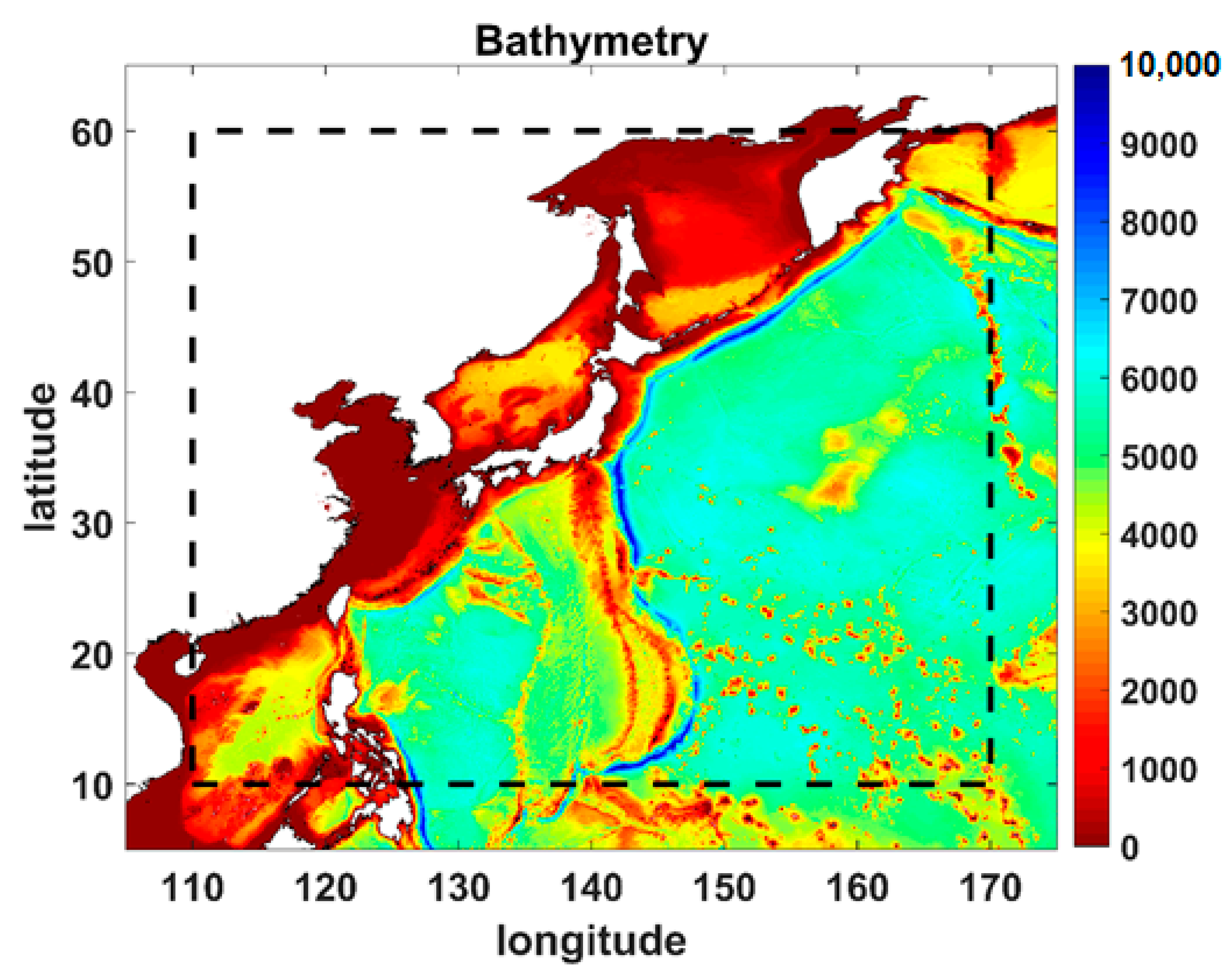
Figure 2.
Comparison of wave characteristics for 2000, such as the mean significant wave height, mean wave direction, and mean wave period, between the AMIP scenario result simulated by WWIII with the CMIP6 marine surface winds (left column) and the ERA5 reanalysis wave dataset (middle column) and the difference between the two (right column).
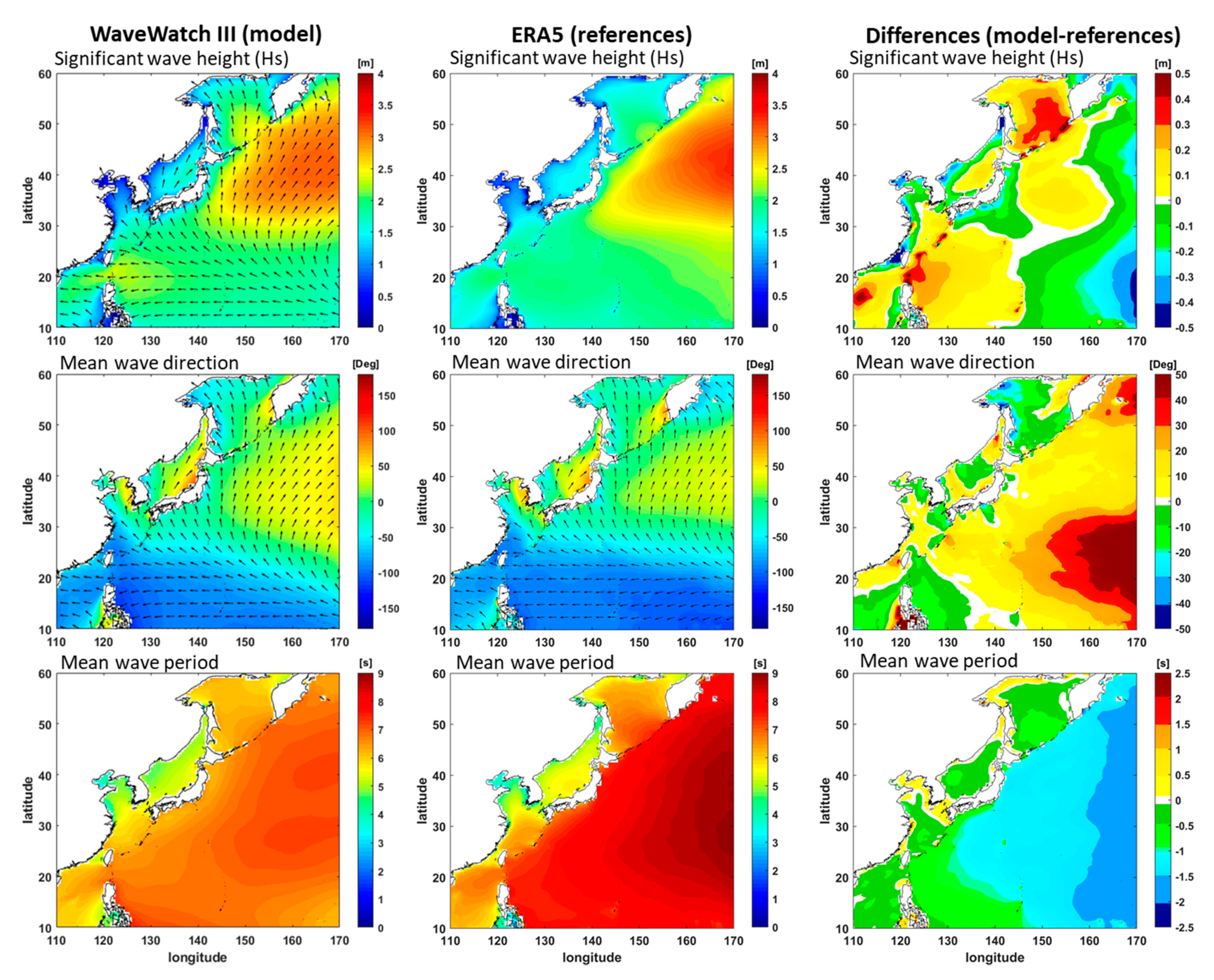
Figure 3.
Mean significant wave height (Hs in m) results for (a) the AMIP scenario result for 2000 and the differences between the results of future scenarios and the AMIP scenario: (b) SSP2-4.5 medium-term, (c) SSP2-4.5 long-term, (d) SSP5-8.5 medium-term, and (e) SSP5-8.5 long-term scenarios.
Figure 3.
Mean significant wave height (Hs in m) results for (a) the AMIP scenario result for 2000 and the differences between the results of future scenarios and the AMIP scenario: (b) SSP2-4.5 medium-term, (c) SSP2-4.5 long-term, (d) SSP5-8.5 medium-term, and (e) SSP5-8.5 long-term scenarios.
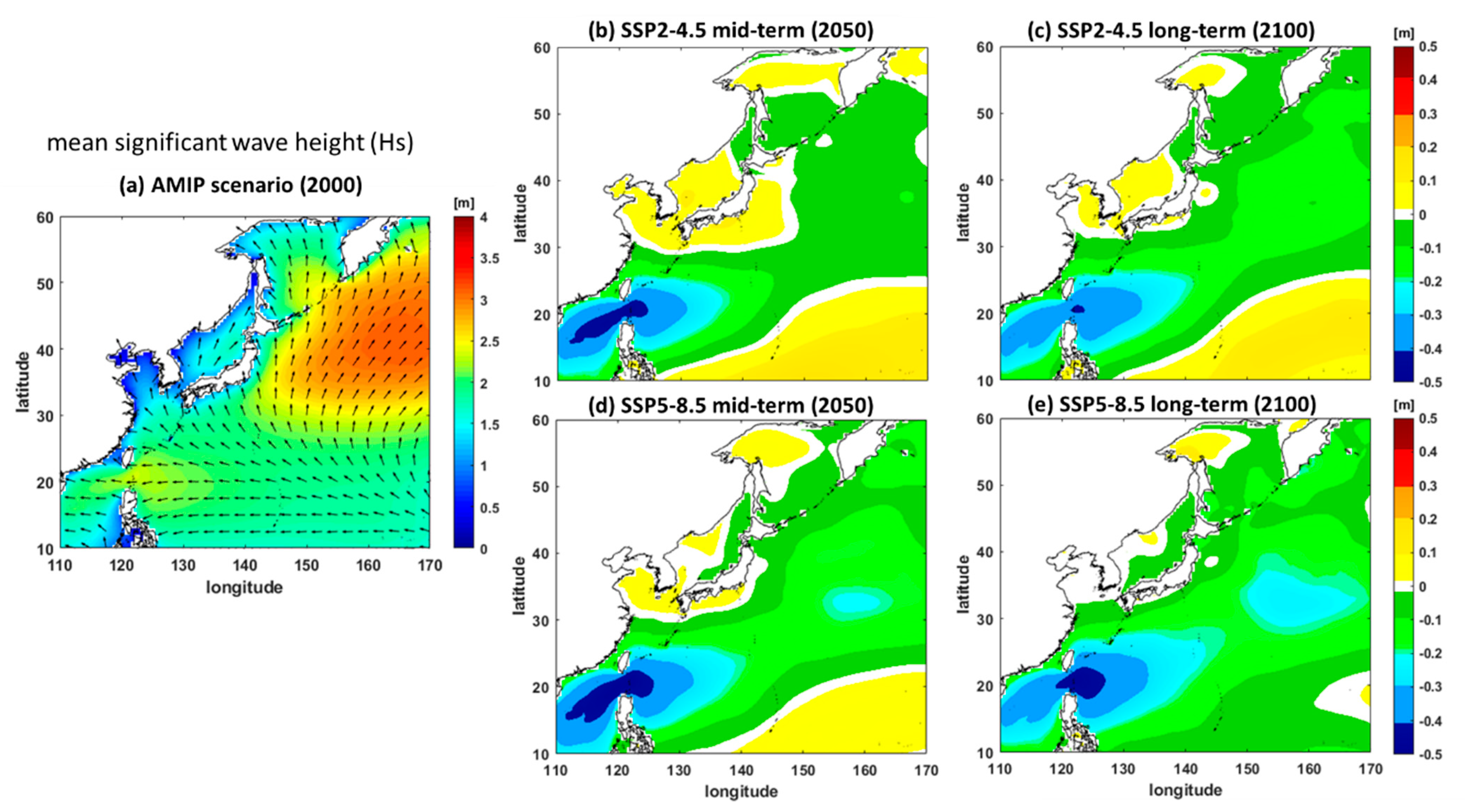
Figure 4.
Mean wave direction ( in degrees) results for (a) the AMIP scenario result for 2000 and the differences between the results of future scenarios and the AMIP scenario: (b) SSP2-4.5 medium-term, (c) SSP2-4.5 long-term, (d) SSP5-8.5 medium-term, and (e) SSP5-8.5 long-term scenarios.
Figure 4.
Mean wave direction ( in degrees) results for (a) the AMIP scenario result for 2000 and the differences between the results of future scenarios and the AMIP scenario: (b) SSP2-4.5 medium-term, (c) SSP2-4.5 long-term, (d) SSP5-8.5 medium-term, and (e) SSP5-8.5 long-term scenarios.
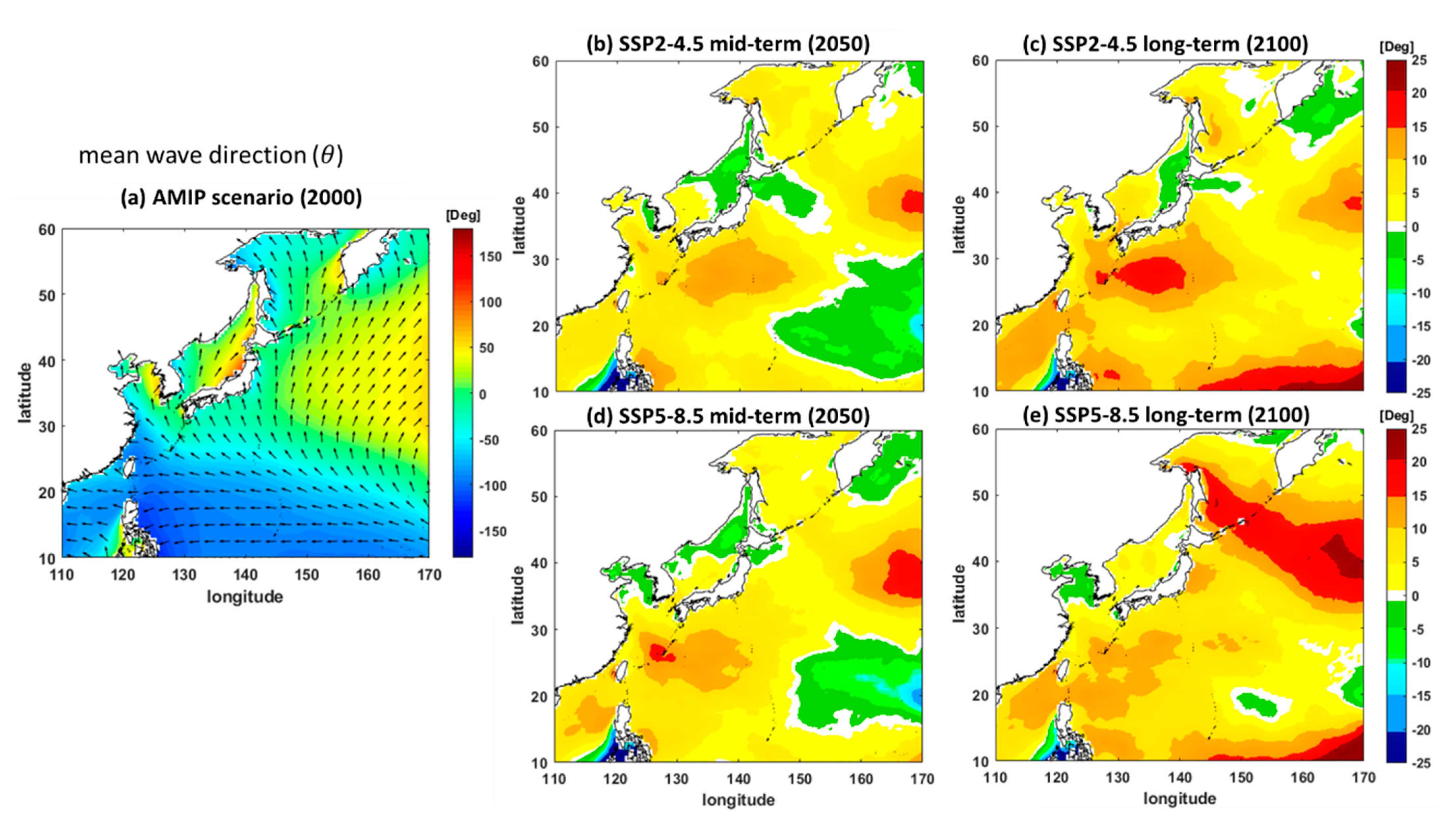
Figure 5.
Mean wave period ( in seconds) results for (a) the AMIP scenario result for 2000 and the differences between the results of future scenarios and the AMIP scenario: (b) SSP2-4.5 medium-term, (c) SSP2-4.5 long-term, (d) SSP5-8.5 medium-term, and (e) SSP5-8.5 long-term scenarios.
Figure 5.
Mean wave period ( in seconds) results for (a) the AMIP scenario result for 2000 and the differences between the results of future scenarios and the AMIP scenario: (b) SSP2-4.5 medium-term, (c) SSP2-4.5 long-term, (d) SSP5-8.5 medium-term, and (e) SSP5-8.5 long-term scenarios.
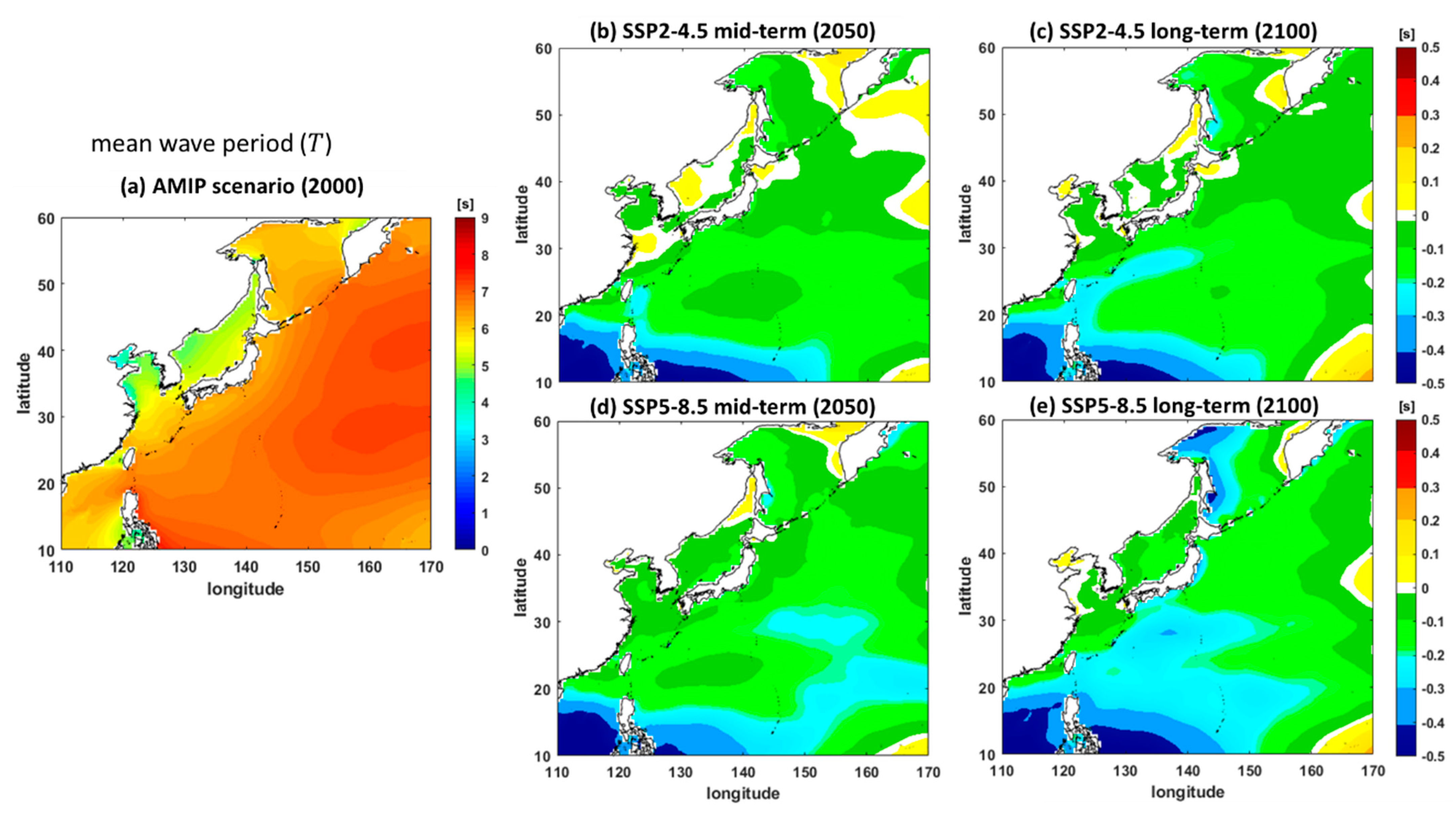
Figure 6.
Annual maximum significant wave height (max. Hs in m) results: (a) AMIP scenario result for 2000, (b) SSP2-4.5 medium-term, (c) SSP2-4.5 long-term, (d) SSP5-8.5 medium-term, and (e) SSP5-8.5 long-term scenarios.
Figure 6.
Annual maximum significant wave height (max. Hs in m) results: (a) AMIP scenario result for 2000, (b) SSP2-4.5 medium-term, (c) SSP2-4.5 long-term, (d) SSP5-8.5 medium-term, and (e) SSP5-8.5 long-term scenarios.

Table 1.
CMIP6 GCMs with a dataset modelled over 3 h used in wind wave modelling.
| Model | Spatial Resolution | Temporal Resolution | Ensemble |
|---|---|---|---|
| BCC-CSM2-MR | 1.12° × 1.125° | 3-h | r1i1p1f1 |
| IPSL-CM6A-LR | 1.267° × 2.5° | r1i1p1f1 | |
| MIROC6 | 1.4° × 1.40625° | r1i1p1f1 | |
| MPI-ESM1-2-HR | 0.9375° × 0.9375° | r1i1p1f1 | |
| MRI-ESM2-0 | 1.12° × 1.125° | r1i1p1f1 | |
| NESM3 | 1.865° × 1.875° | r1i1p1f1 | |
| CNRM-CM6-1 | 1.4° × 1.40625° | r1i1p1f2 | |
| CNRM-ESM2-1 | 1.4° × 1.40625° | r1i1p1f2 |
Table 2.
Summary of numerical experiments with model setups and surface winds.
| Year | Scenario | Surface Wind (3 hourly) | WWIII Source Terms | Remarks | |||
| Wind Input (Sin) | Nonlinear Wave Interaction (Snl) | White Capping Dissipation (Sds) | Depth-induced Breaking (Sdb) | ||||
| 2000 | historical | AMIP | linear input (Cavaleri and Malanotte-Rizzli [41]) | discrete interaction approximation (DIA) | ST4 (Ardhuin et al. [45]) | (Battjes and Janssen [44]) | Bathymetry: GEBCO 15 arc-second data Shoreline: GSHHG |
| 2050 | SSP2-4.5 | 8 ensembles from 8 GCMs (Table 1) | |||||
| SSP5-8.5 | |||||||
| 2100 | SSP2-4.5 | ||||||
| SSP5-8.5 | |||||||
Publisher’s Note: MDPI stays neutral with regard to jurisdictional claims in published maps and institutional affiliations. |
© 2021 by the authors. Licensee MDPI, Basel, Switzerland. This article is an open access article distributed under the terms and conditions of the Creative Commons Attribution (CC BY) license (https://creativecommons.org/licenses/by/4.0/).
Share and Cite
MDPI and ACS Style
Badriana, M.R.; Lee, H.S. Multimodel Ensemble Projections of Wave Climate in the Western North Pacific Using CMIP6 Marine Surface Winds. J. Mar. Sci. Eng. 2021, 9, 835. https://doi.org/10.3390/jmse9080835
AMA Style
Badriana MR, Lee HS. Multimodel Ensemble Projections of Wave Climate in the Western North Pacific Using CMIP6 Marine Surface Winds. Journal of Marine Science and Engineering. 2021; 9(8):835. https://doi.org/10.3390/jmse9080835
Chicago/Turabian StyleBadriana, Mochamad Riam, and Han Soo Lee. 2021. "Multimodel Ensemble Projections of Wave Climate in the Western North Pacific Using CMIP6 Marine Surface Winds" Journal of Marine Science and Engineering 9, no. 8: 835. https://doi.org/10.3390/jmse9080835
Note that from the first issue of 2016, this journal uses article numbers instead of page numbers. See further details here.