Full Support for Efficiently Mining Multi-Perspective Declarative Constraints from Process Logs ^†

Abstract

Declarative process management has emerged as an alternative solution for describing flexible workflows. In turn, the modelling opportunities with languages such as Declare are less intuitive and hard to implement. The area of process discovery covers the automatic discovery of process models. It has been shown that the performance of process mining algorithms, particularly when considering the multi-perspective declarative process models, are not satisfactory. State-of-the-art mining tools do not support multi-perspective declarative models at this moment. We address this open research problem by proposing an efficient mining framework that leverages the latest big data analysis technology and builds upon the distributed processing method MapReduce. The paper at hand further completes the research on multi-perspective declarative process mining by extending our previous work in various ways; in particular, we introduce algorithms and descriptions for the full set of commonly accepted types of MP-Declare constraints. Additionally, we provide a novel implementation concept allowing an easy introduction and discovery of customised constraint templates. We evaluated the mining performance and effectiveness of the presented approach on several real-life event logs. The results highlight that, with our efficient mining technique, multi-perspective declarative process models can be extracted in reasonable time.

1. Introduction

The research field of process mining refers to the automated discovery, conformance checking and enhancement of business process models. Automated process discovery generates process models from digitally provided event logs consisting of traces, such that each trace corresponds to one execution of the recorded process. Each event in a trace consists of an event class (i.e., the activity to which the event corresponds) and a timestamp. However, further information may also be available such as the originator that performed a certain activity as well as data values in the form of attribute–value pairs. Process mining is especially relevant for the analysis of processes that are often referred to as flexible, unstructured or knowledge-intense [1]. Applying traditional process mining approaches that extract procedural process models result in models that are colloquially called Spaghetti models due to their complex und unreadable structure [2]. The results of process mining can alternatively be represented as declarative process models, i.e., rules for directly representing the causality of the behaviour [3]. The advantages of declarative languages such as Declare [4] or DPIL [5] have been emphasised in the literature. It is also well known that behaviour is typically intertwined with dependencies upon value ranges of data parameters and resource characteristics [6]. An example sheds some light into this complex issue. Let us assume a review activity must be performed. Both novices and experts of a certain team are eligible to perform this task. However, if a novice is executing it, it is required that a second person is double-checking the result. Thus, the activity “double-checking” only has to be executed when novices perform the review step. Here, the resource perspective influences the behavioural perspective. Therefore, Declare has been extended towards Multi-Perspective Declare (MP-Declare) [7]. The relative strengths and weaknesses of different declarative process discovery algorithms are discussed in the literature [8,9,10]. In summary, state-of-the-art mining tools such as MINERful [11,12] and DeclareMiner [13] do not support MP-Declare at this moment. In particular, the discovery of constraints that impose additional statements on data values or ranges of data values, respectively, is an issue. In [14,15], first approaches to enable the discovery of MP-Declare constraints based on SQL and relational databases have been proposed. However, it has not been investigated how this complex mining task can be performed in an efficient way.

In our previous work [16], we first addressed this open research problem by proposing an efficient mining framework for discovering MP-Declare models that leverages latest big data analysis technology and builds upon the distributed processing method MapReduce. We introduced a preliminary subset of parallelisable algorithms for discovering commonly used types of MP-Declare constraints. The paper at hand further completes the research on MP-Declare mining by extending our previous work [16] in various ways:

(i)

We introduce algorithms and descriptions for the full set of commonly accepted types of MP-Declare constraints.

(ii)

The conceptual architecture of the implementation has been reworked such that new types of constraints can be easily defined and extracted by the user.

(iii)

We provide a more detailed description of the conceptual approach as well as the implemented protoype.

(iv)

Related work is discussed more thoroughly.

We evaluated the mining performance and effectiveness of the presented approach on several real-life event logs. The results highlight that, with our efficient mining technique, multi-perspective declarative process models can be extracted in reasonable duration.

The paper is structured as follows. Section 2 discusses related work. Section 3 introduces the language and semantics of MP-Declare as well as basic mining metrics. Section 4 describes the distributed framework we propose to speed up multi-perspective declarative process discovery. In particular, we describe the whole set of algorithms to extract commonly used types of declarative constraints. Section 5 describes the implementation of our approach as well as the evaluation of our technique with real-life cases. Section 7 concludes the paper.

2. Related Work

Several approaches have been proposed for the discovery of declarative process models. The relative strengths and weaknesses of different declarative process discovery algorithms are discussed in the literature [8,9,10]. In [17], the authors presented an approach that allows the user to select from a set of predefined Declare templates the ones to be used for the discovery. Other approaches to improve the performances of the discovery task are presented in [18,19]. Additionally, there are post-processing approaches that aim at simplifying the resulting Declare models in terms of redundancy elimination [20,21], consistency checking [21,22] and disambiguation [23].

Other approaches for the discovery of Declare constraints have been presented in [24,25,26]. In [24], the authors presented the Evolutionary Declare Miner, which implements the discovery task using a genetic algorithm. The work in [25,26] describes the usage of inductive logic programming techniques to mine models expressed as a SCIFF first-order logic theory, consisting of a set of implication rules named Social Integrity Constraints (ICs). Finally, the learned theory is translated into the Declare notation.

An approach similar to the SQL-based one is presented in [27] and is based on temporal logic query checking. In [28], the authors defined Timed Declare, an extension of Declare that relies on timed automata. In [29], an approach for analysing event logs with Timed Declare is proposed. The DPILMiner [30], the RALphMiner [31] and the team compositions miner [32] exploit discovery approaches to incorporate the resource perspective and to mine for a set of predefined resource assignment constraints. In [33], the authors introduced for the first time a data-aware semantics for Declare and [34] first covered the data perspective in declarative process discovery, although this approach only allows for the discovery of discriminative activation conditions. The work in [14,15] proposes the first approach to enable the discovery of MP-Declare constraints by querying event logs given in relational databases with SQL. Hence, event logs first need to be imported into a relational database and the templates of MP-Declare are mapped to SQL queries. Existing research on SQL-based MP-Declare mining focuses on the description of effectiveness, however, a performance evaluation has not been described.

Furthermore, MP-Declare models are supported in the context of conformance checking [35], trace generation [36] and execution [37]. The execution engine builds on a classification strategy for different constraint types and a transformation component into the execution language Alloy that is used to solve SAT problems. Here, a modelling and execution prototype has been implemented as well.

In recent work [16,38], the authors presented a distributed approach for mining MP-Declare process models based on MapReduce. The paper at hand extends this work by providing algorithms and descriptions for the full set of commonly accepted types of MP-Declare constraints as well as an in-depth description of the implemented prototype. Furthermore, the conceptual architecture of the implementation has been reworked such that new types of constraints can be easily defined and extracted by the user.

3. Preliminaries

In this section, we describe the basic concepts of of multi-perspective declarative process modelling and introduce basic metrics of declarative process mining. Further on, we introduce in the basic concepts of MapReduce as scaffolding computation model.

3.1. Multi-Perspective, Declarative Process Modelling

Declarative process models are strong in representing the behaviour of flexible business processes. Declarative process modelling languages such as Declare [39] describe a set of constraints that must be satisfied throughout the process execution. Constraints are instances of predefined templates. Templates are patterns that define parameterised classes of properties. The semantics of such templates are typically formalised using formal logics such as Linear Temporal Logic over finite traces (LTL${}_f$) [40].

The main shortcoming of existing languages such as Declare is the fact that templates are not capable of modelling the connection between the temporal flow and other perspectives of a process. Consider the example of a loan application process where it should be possible to specify constraints such as the following:

• Activation conditions: When a loan is requested and account balance > 4000 EUR, the loan must subsequently be granted.
• Correlation conditions: When a loan is requested, the loan must subsequently be granted and amount requested = amount granted.
• Target conditions: When a loan is requested, the loan must subsequently be granted by a specific member of the financial board.
• Temporal conditions: When a loan is requested, the loan must subsequently be granted within the next 30 days.

Traditional Declare only allows for defining single-perspective constraints that relate activities without considering other process perspectives such as data values and resources. Here, the $\mathbf{F}$, $\mathbf{X}$, $\mathbf{G}$, and $\mathbf{U}$ LTL${}_f$ future operators have the following semantics: formula $\mathbf{F}{\psi }_1$ means that ${\psi }_1$ holds sometime in the future; $\mathbf{X}{\psi }_1$ means that ${\psi }_1$ holds in the next position; $\mathbf{G}{\psi }_1$ means that ${\psi }_1$ holds forever in the future; and ${\psi }_1\mathbf{U}{\psi }_2$ means that sometime in the future ${\psi }_2$ will hold and until that moment ${\psi }_1$ holds (with ${\psi }_1$ and ${\psi }_2$ LTL${}_f$ formulas). The $\mathbf{O}$, $\mathbf{Y}$ and $\mathbf{S}$ LTL${}_f$ past operators have the following meaning: $\mathbf{O}{\psi }_1$ means that ${\psi }_1$ holds sometime in the past; $\mathbf{Y}{\psi }_1$ means that ${\psi }_1$ holds in the previous position; and ${\psi }_1\mathbf{S}{\psi }_2$ means that ${\psi }_1$ has held sometime in the past and since that moment ${\psi }_2$ holds.

The response constraint $\mathbf{G}(A\to \mathbf{F}B)$, for example, defines that if Aoccurs, B must eventually follow. Hence, this constraint is satisfied in traces such as ${\mathbf{t}}_1$ = $\langle A,A,B,C\rangle$, ${\mathbf{t}}_2=\langle B,B,C,D\rangle$, and ${\mathbf{t}}_3=\langle A,B,C,B\rangle$, but not for ${\mathbf{t}}_4=\langle A,B,A,C\rangle$ because the second occurrence of A is not followed by a B. In ${\mathbf{t}}_2$, it is so-called vacuously satisfied [41], in a trivial way, because A never occurs.

An activation activity of a constraint in a trace is an activity whose execution imposes some obligations on the execution of other activities (the so-called target activities) in the same trace (see  

Table 1. Semantics for MP-Declare constraints in LTL${}_f$.

Template	LTL${}_{\mathbf{f}}$ Semantics
existence$(A)$	$\top \to \mathbf{F}(e(A)\begin{array}{c}\hfill \wedge {\phi }_a(\overrightarrow{x})\end{array})\vee \mathbf{O}(e(A)\begin{array}{c}\hfill \wedge {\phi }_a(\overrightarrow{x})\end{array})$
responded existence$(A, B)$	$\mathbf{G}((A\begin{array}{c}\hfill \wedge {\phi }_a(\overrightarrow{x})\end{array})\to (\mathbf{O}(B\begin{array}{c}\hfill \wedge {\phi }_c(\overrightarrow{x},\overrightarrow{y})\wedge {\phi }_t(\overrightarrow{y})\end{array})\vee \mathbf{F}(B\begin{array}{c}\hfill \wedge {\phi }_c(\overrightarrow{x},\overrightarrow{y})\wedge {\phi }_t(\overrightarrow{y})\end{array})))$
response$(A, B)$	$\mathbf{G}((A\begin{array}{c}\hfill \wedge {\phi }_a(\overrightarrow{x})\end{array})\to \mathbf{F}(B\begin{array}{c}\hfill \wedge {\phi }_a(\overrightarrow{x})\wedge {\phi }_c(\overrightarrow{x},\overrightarrow{y})\wedge {\phi }_t(\overrightarrow{y})\end{array}))$
alternate response$(A, B)$	$\mathbf{G}((A\begin{array}{c}\hfill \wedge {\phi }_a(\overrightarrow{x})\end{array})\to \mathbf{X}(\neg (A\begin{array}{c}\hfill \wedge {\phi }_a(\overrightarrow{x})\end{array})\mathbf{U}(B\begin{array}{c}\hfill \wedge {\phi }_c(\overrightarrow{x},\overrightarrow{y})\wedge {\phi }_t(\overrightarrow{y})\end{array}))$
chain response$(A, B)$	$\mathbf{G}((A\begin{array}{c}\hfill \wedge {\phi }_a(\overrightarrow{x})\end{array})\to \mathbf{X}(B\begin{array}{c}\hfill \wedge {\phi }_a(\overrightarrow{x})\wedge {\phi }_c(\overrightarrow{x},\overrightarrow{y})\wedge {\phi }_t(\overrightarrow{y})\end{array}))$
precedence$(A, B)$	$\mathbf{G}((B\begin{array}{c}\hfill \wedge {\phi }_a(\overrightarrow{x})\end{array})\to \mathbf{O}(A\begin{array}{c}\hfill \wedge {\phi }_a(\overrightarrow{x})\wedge {\phi }_c(\overrightarrow{x},\overrightarrow{y})\wedge {\phi }_t(\overrightarrow{y})\end{array}))$
alternate precedence$(A, B)$	$\mathbf{G}((B\begin{array}{c}\hfill \wedge {\phi }_a(\overrightarrow{x})\end{array})\to \mathbf{Y}(\neg (B\begin{array}{c}\hfill \wedge {\phi }_a(\overrightarrow{x})\end{array})\mathbf{S}(A\begin{array}{c}\hfill \wedge {\phi }_c(\overrightarrow{x},\overrightarrow{y})\wedge {\phi }_t(\overrightarrow{y})\end{array}))$
chain precedence$(A, B)$	$\mathbf{G}((B\begin{array}{c}\hfill \wedge {\phi }_a(\overrightarrow{x})\end{array})\to \mathbf{Y}(A\begin{array}{c}\hfill \wedge {\phi }_a(\overrightarrow{x})\wedge {\phi }_c(\overrightarrow{x},\overrightarrow{y})\wedge {\phi }_t(\overrightarrow{y})\end{array}))$
co existence$(A, B)$	$responded existence(A, B)\wedge responded existence(B, A)$
succession$(A, B)$	$response(A, B)\wedge precedence(A, B)$
alternate succession$(A, B)$	$alternate response(A, B)\wedge alternate precedence(A, B)$
chain succession$(A, B)$	$chain response(A, B)\wedge chain precedence(A, B)$
not responded existence$(A, B)$	$\mathbf{G}((A\begin{array}{c}\hfill \wedge {\phi }_a(\overrightarrow{x})\end{array})\to \neg (\mathbf{O}(B\begin{array}{c}\hfill \wedge {\phi }_c(\overrightarrow{x},\overrightarrow{y})\wedge {\phi }_t(\overrightarrow{y})\end{array})\vee \mathbf{F}(B\begin{array}{c}\hfill \wedge {\phi }_c(\overrightarrow{x},\overrightarrow{y})\wedge {\phi }_t(\overrightarrow{y})\end{array})))$
not response$(A, B)$	$\mathbf{G}((A\begin{array}{c}\hfill \wedge {\phi }_a(\overrightarrow{x})\end{array})\to \neg \mathbf{F}(B\begin{array}{c}\hfill \wedge {\phi }_a(\overrightarrow{x})\wedge {\phi }_c(\overrightarrow{x},\overrightarrow{y})\wedge {\phi }_t(\overrightarrow{y})\end{array}))$
not precedence$(A, B)$	$\mathbf{G}((B\begin{array}{c}\hfill \wedge {\phi }_a(\overrightarrow{x})\end{array})\to \neg \mathbf{O}(A\begin{array}{c}\hfill \wedge {\phi }_a(\overrightarrow{x})\wedge {\phi }_c(\overrightarrow{x},\overrightarrow{y})\wedge {\phi }_t(\overrightarrow{y})\end{array}))$
not chain response$(A, B)$	$\mathbf{G}((A\begin{array}{c}\hfill \wedge {\phi }_a(\overrightarrow{x})\end{array})\to \neg \mathbf{X}(B\begin{array}{c}\hfill \wedge {\phi }_a(\overrightarrow{x})\wedge {\phi }_c(\overrightarrow{x},\overrightarrow{y})\wedge {\phi }_t(\overrightarrow{y})\end{array}))$
not chain precedence$(A, B)$	$\mathbf{G}((B\begin{array}{c}\hfill \wedge {\phi }_a(\overrightarrow{x})\end{array})\to \neg \mathbf{Y}(A\begin{array}{c}\hfill \wedge {\phi }_a(\overrightarrow{x})\wedge {\phi }_c(\overrightarrow{x},\overrightarrow{y})\wedge {\phi }_t(\overrightarrow{y})\end{array}))$
not co existence$(A, B)$	$not responded existence(A, B)\wedge not responded existence(B, A)$
not succession$(A, B)$	$not response(A, B)\wedge not precedence(A, B)$
not chain succession$(A, B)$	$not chain response(A, B)\wedge not chain precedence(A, B)$

). A is an activation activity for the response constraint $\mathbf{G}(A\to \mathbf{F}B)$ and B is a target, because performing A forces B to be executed, at some point in the future. An activation of a constraint leads to a fulfillment or to a violation. Consider, $\mathbf{G}(A\to \mathbf{F}B)$. In trace ${\mathbf{t}}_1$, the constraint is activated and fulfilled twice; however, in trace ${\mathbf{t}}_3$, it is activated and fulfilled only once. In trace ${\mathbf{t}}_4$, it is activated twice and the second activation leads to a violation (B does not occur subsequently).

The necessity for defining such multi-perspective coherencies led to the definition of a multi-perspective extension of Declare (called MP-Declare) [35]. The semantics of MP-Declare build on the term of payload of an event. $e(activity)$ identifies the occurrence of an event to distinguish it from the activity name. At the time of a certain event e, its attributes $x_1,\dots ,x_m$ have certain values. $p_{activity}^e=(va{l}_{x1},\dots ,va{l}_{xn})$ represents its payload. To denote the projection of the payload $p_A^e=(x_1,\dots ,x_n)$ over attributes $x_1,\dots ,x_m$ with $m⩽n$, the notation $p_A^e[x_1,\dots ,x_m]$ is used. For instance, $p_{ApplyForTrip}^e\left[Resource\right]$=SS is the projection of the attribute Resource in the event description. Moreover, the n-ples of attributes $x_i$ are given as $\overrightarrow{x}$. Hence, the templates in MP-Declare extend the traditional version of Declare with further conditions and constraints on event attributes. In particular, given the events $e(A)$ and $e(B)$ with payloads $p_A^e=(x_1,\dots ,x_n)$ and $p_B^e=(y_1,\dots ,y_n)$, the activation condition${\phi }_a$, the correlation condition${\phi }_c$, and the target condition${\phi }_t$ are specified. The activation condition is part of the activation ${\varphi }_a$, whereas the correlation and target conditions are part of the target ${\varphi }_t$, according to their respective time of execution and evaluation. The activation condition is a fact that must be valid when the activation happens. For a response constraint, the activation condition has the shape ${\phi }_a(x_1,\dots ,x_n)$, meaning that the proposition ${\phi }_a$ over $(x_1,\dots ,x_n)$ must hold true. The correlation condition must be valid when the target happens, and it relates the payloads of the activation and the target event. It has the shape ${\phi }_c(x_1,\dots ,x_m,y_1,\dots ,y_m)$ with $m⩽n$, where ${\phi }_c$ is a formula on the variables of both the payload of $e(A)$ and the payload of $e(B)$. Target conditions express conditions on the values of the attributes that are registered at the moment wherein the target activity occurs. They have the shape ${\phi }_t(y_1,\dots ,y_m)$ with $m⩽n$, where ${\phi }_t$ is a propositional formula involving variables in the payload of $e(B)$.

3.2. Metrics for Mining MP-Declare Models

In this section, we explain the metrics that are used to distinguish between constraints that are fulfilled in the event log and constraints that are rarely satisfied. These metrics are called support and confidence.

Evaluation the given constraint templates provides for every possible combination of values for the free variables in the templates the number of satisfactions in the examined log. Based on the number of satisfactions, two metrics, Support and Confidence, are calculated, which express the probability of a concrete constraint to be valid during process execution. Here, Support is defined as the number of fulfilments of a constraint divided by the number of occurrences of the condition of a constraint. The Confidence metric scales the support by the fraction of traces in the log where the activation condition is satisfied. Constraints are considered valid if their Support and Confidence values are above a certain threshold. In the work at hand, we consider two specifications of support that have been defined in the literature, namely the event-based support [12] and the trace-based support [17]. As defined in [12], we denote the set of events in a trace $\mathbf{t}$ of an event log L that fulfil an LTL${}_f$ formula $\psi$ as ${\vDash }_{\mathbf{t}}^e (\psi )$. The set of all events in the log L that fulfil $\psi$ are given as ${\vDash }_L^e (\psi )$. Given a constraint $\Xi$ comprising activation ${\varphi }_a$ and target ${\varphi }_t$, the event-based support ${\mathcal{S}}_L^e$ and the event-based confidence ${\mathcal{C}}_L^e$ as follows:

$${\mathcal{S}}_L^e=\frac{{\displaystyle \sum _{i=1}^{\left|L\right|}}\left|{\vDash }_{{\mathbf{t}}_i}^e (\Xi )\right|}{\left|{\vDash }_L^e ({\varphi }_a)\right|}$$

(1)

$${\mathcal{C}}_L^e=\frac{{\mathcal{S}}_L^e\times \left|{\vDash }_L^e ({\varphi }_a)\right|}{\left|L\right|}$$

(2)

3.3. MapReduce

3.3.1. Origin

MapReduce was originally introduced back in 2004 by Jeffrey Dean and Sanjay Ghemawat [42] to handle the storage and processing of Google Inc.’s internal datasets, which exceeded the size of normal datasets (BigData) and thus are not applicable with contemporary processing methods. These data are usually distributed over several nodes within a network of hard drives. The MapReduce programming model helps to write frugal code snippets in terms of abstracting from low-level layers like network communication, parallelisation, node failure, etc. The wide-ranging application use cases, e.g., large-scale machine learning problems, analysing web pages and indexing the Word Wide Web for Google’s web search service, shows the versatility of MapReduce. Since then, MapReduce has entered and solved many issues in a variety of application domains. In this paper, we carry the list of use-cases forward in terms of an efficient framework for discovering multi-perspective declarative process models within the field of Business Process Management.

3.3.2. Implementations

There are a couple of confounding artefacts referring to the same terminology, i.e., MapReduce (or map and reduce), but include different concepts. To avoid misunderstandings, the two main representatives are differentiated here.

• MapReduce. Referring to Google’s original paper [42] or Hadoop [43], the open source de-facto standard implementation in Java, MapReduce, implies two functions, namely Map (a parallel transformation) and Reduce (a parallel aggregation). For the sake of performance with large datasets, these implementations include an intermediate shuffle or group phase.
• Map and Reduce in Functional Programming. Functional Programming languages or frameworks, such as Haskell, Java (includes functional concepts since Version 1.8) or Spark, also use the terms map and reduce, but are different from the MapReduce concepts mentioned above. For instance, in functional programming, users specify the semantic logic in a declarative way rather than the control flow [44].

However, we specify the functionality of process model discovery in an abstract way, so that it can be migrated to any implementation, e.g. Apache’s Hadoop [38] or Java (cf. Section 5).

3.3.3. Functionality

In this section, we explain the basic principle of MapReduce by means of the typical word-count example. As stated, this can be applied to several implementations and serves as fundamental basis for the remainder of the paper.

The input of the map-function is the text whose words are going to be counted. As we want to count the words (not characters or something else), we have to split the sentences or text by whitespaces, to receive the whole text separated by words. The map-function produces key–value pairs and for our simple example each word builds the key of a single key–value pair with the value 1 (e.g., (Process, 1)). The reduce-function obtains then key–value pairs, whose values are aggregated to identical keys (during the shuffling or grouping phase), e.g., each value 1 of the three key–value pairs (Process, 1) are aggregated to (Process, [1, 1, 1]) in the example below. The Reducer finally processes the list of values, for instance sums up the elements, e.g., (Process, 3).

Full Example:

Input:Declarative Process Mining discovers Declarative Process Models, used in Business Process Management.

Mapping:

(Declarative, 1), (Process, 1), (Mining, 1), (discovers, 1), (Devlarative, 1), (Process, 1), (Models,, 1), (used, 1), (in, 1), (Business, 1), (Process, 1), (Management, 1)

Shuffling:

(Declarative, [1, 1]), (Process, [1, 1, 1]), (Mining, 1), (discovers, 1), (Models,, 1), (used, 1) (in, 1), (Business, 1), (Management, 1)

Reducing:

(Declarative, 2), (Process, 3), (Mining, 1), (discovers, 1), …

In a nutshell, the map-function applies logic to its input and produces key–value pairs based on the logic. In sophisticated frameworks, a shuffle or group stage follows to do a pre-aggregation for performance issues. The reduce-function receives the prepared key–value pairs and again applies specific logic to it.

4. Map-Reduce for Declarative Process Mining

In this section, we describe an efficient framework for discovering MP-Declare constraints. After giving insights into the internal infrastructure, we explain the parallelisable discovery algorithms for commonly used MP-Declare constraints that are used to discover models under consideration of further perspectives.

4.1. Architecture and Infrastructure

The basic idea of the algorithm builds upon the MapReduce computation model. One key advantage is the inbuilt opportunity for executing the calculations in parallel, leading to an enormous performance boost. At first, the scaffolding of the MapReduce algorithm is described briefly by means of relational constraints with respect to the discovery of a process model described below. In the next section, we use an example log containing two traces defined in Equation (3). For the sake of comprehensibility, we use in this case a single-perspective example to outline the calculation steps.

$$t_0=\langle a,b,b,c\rangle t_1=\langle a,c,d\rangle$$

(3)

To compute the support and confidence metrics, two MapReduce jobs are required, MR-I and MR-II (cf. Figure 1).

4.1.1. MR-I

In the map-phase of MR-I, key–value pairs are created from the locally provided event data, i.e., a single trace of a log file. Each of the key–value pairs is assigned to a number for further processing. In the case of process discovery, this number is always 1. The challenge is to generate these key–value pairs in order to address the logic for the MP-Declare constraints.

Example 1.

Given a trace $t_0=\langle a,b,b,c\rangle$, consider the response template, i.e., whenever an event $e_1$ occurs, the event $e_2$ must follow ($response(e_1,e_2)$). The trace $t_0$ is therefore mapped to five different key–value pairs in the map phase: $((a,b),1),((a,c),1),((b,b),1),((b,c),1),((b,c),1)$. The keys are exactly those event pairs which fulfil the response template: a is followed by b and c, the first b is followed by c and the second b, which is again followed by c. Note that a constraint can only be fulfilled once per trace, e.g. $response(a,b)$ is fulfilled only by the first event b. The underlying mapping algorithm containing the logic for all constraint templates is described in Section 4.2.

The reduce-phase finally obtains the key–value pairs that have been produced. The reduce-function must be declared by the user once again. In the case of constraint checking, this phase depicts a summation of values. To continue the example above, the result of the reducer with trace $t_0$ is: $((a,b),1),((a,c),1),((b,b),1),((b,c),2)$.

$\sigma$-Function

The support metric is defined as the number of fulfilments of a constraint divided by the number of occurrences of the activation. The MR-I job in the example above calculates exactly the number of fulfilments, thus the numerator of the support formula. In the following, we use a function ${\sigma }_{\gamma }:E\times E\to \mathbb{N}$, where E are events, for describing this figure, e.g., in $t_0$: ${\sigma }_{response}(b,c)=2$. $\gamma$ denotes a constraint template like $response$ or $chainResponse$.

$\eta$-Function

To calculate the support of a constraint, the number of occurrences of the activation is necessary. If the event that fulfils a constraint occurs after the activation event (future constraining constraints), this is the first event in the constraint template, e.g., b in the constraint $response(b,c)$. In the reverse case, where the event that fulfils a constraint occurs before the activation event (history-based constraints), event c would be taken into account. We define the number of occurrences of events as $\eta :E\to \mathbb{N}$, for instance in trace $t_0$: $\eta (b)=2$. To obtain the correct values for the $\eta$-function, for each event e in the trace a key–value pair, $(e,1)$ is additionally emitted in the map phase, e.g., for $t_0$, $(a,1),(b,1),(b,1),(c,1)$, which is reduced to $(a,1),(b,2),(c,1)$.

$ϵ$-Function

A third value is necessary for determining the confidence, namely the amount of traces in which a given event occurs. We introduce the function $ϵ:E\to \mathbb{N}$, which holds this information. Taking into account the second trace $t_1$ (cf. Equation (3)), MR-I outputs $ϵ(c)=2$ or $ϵ(d)=1$, as c occurs in $t_0$ and $t_1$, whereas d occurs in $t_1$ solely. Transferring this to MR-I, for each unique event e, a key–value pair $(e,1)$ has to be produced, neglecting multiple occurrences of events, e.g., for trace $t_0$: $(a,1),(b,1),(c,1)$.

Table 2. Output Mapper MR-I [16].

Trace	${\mathbf{\sigma }}_{\mathit{R}}$		${\mathbf{\sigma }}_{\mathit{CR}}$	$\mathbf{\eta }$	$\mathbf{ϵ}$
a,b,b,c	ab,1	bc,1	ab,1	a,1	a,1
	ac,1		bb,1	b,1	b,1
	bb,1		bc,1	b,1	c,1
	bc,1			c,1
a,c,d	ac,1		ac,1	a,1	a,1
	ad,1		cd,1	c,1	c,1
	cd,1			d,1	d,1

and

Table 3. Output Reducer MR-I [16].

${\mathbf{\sigma }}_{\mathit{R}}$		${\mathbf{\sigma }}_{\mathit{CR}}$		$\mathbf{\eta }$	$\mathbf{ϵ}$
ab,1	bc,2	ab,1	ac,1	a,2	a,2
ac,2	ad,1	bb,1	cd,1	b,2	b,1
bb,1	cd,1	bc,1		c,2	c,2
				d,1	d,1

show the complete result of MR-I for the input log (cf. Equation (3)) considering two constraint templates: response and chainResponse. The output of all mappers serves as the input for the reducers.

4.1.2. MR-II

Two MapReduce jobs are performed where the event log only serves as input for the first MapReduce job. The output values of MR-I are used in MR-II to calculate support and confidence. Note that these calculations had to be extracted to a separate job because every single trace of the provided log needs to be tackled first in MR-I in order to obtain the $\sigma$-, $\eta$- and $ϵ$-functions. This makes MR-II mandatory; however, with a look on the performance, support and confidence can be computed in parallel again.

Using the functions introduced above, the support of a (future constraining) constraint $response(b,c)$ can be computed as ${\mathcal{S}}_R(b,c)=\frac{{\sigma }_R(b,c)}{\eta (b)}=\frac{2}{2}=1$ (cf. Equation (4)), thus as the fraction between the fulfilments of the constraint and the amount of its activations.

$${\mathcal{S}}_{FC}(e_1,e_2)=\frac{\sigma (e_1,e_2)}{\eta (e_1)}$$

(4)

$${\mathcal{S}}_{BC}(e_1,e_2)=\frac{\sigma (e_1,e_2)}{\eta (e_2)}$$

(5)

The confidence of a (future constraining) constraint for an event pair $(e_1,e_2)$ is the product of the support of $(e_1,e_2)$ with the ratio between the amount of traces in the log in which event $e_1$ occurs (or $e_2$ in case of history-based constraints) and the total number of traces in the log, denoted as $\left|l\right|$ in Equation (6).

$${\mathcal{C}}_{FC}(e_1,e_2)={\mathcal{S}}_{FC}(e_1,e_2)·\frac{ϵ(e_1)}{\left|l\right|}$$

(6)

$${\mathcal{C}}_{BC}(e_1,e_2)={\mathcal{S}}_{BC}(e_1,e_2)·\frac{ϵ(e_2)}{\left|l\right|}$$

(7)

In the running example, the confidence of the constraint $response(b,c)$ is calculated as ${\mathcal{C}}_R(b,c)={\mathcal{S}}_R(b,c)·(\frac{ϵ(b)}{\left|l\right|})=1·\frac{1}{2}=0.5$.

In terms of MapReduce, the MR-II is structured rather trivial. In the map-phase, the output of MR-I is conducted directly to the reducer neglecting $\eta$ and $ϵ$, i.e., all key–value pairs of the $\sigma$-function of all constraints are emitted and obtained by the reducer. The reduce-function then consults the DB to look up the relevant $\eta$- and $ϵ$-value for a given key and calculates the corresponding support and confidence values (according to Equations (4)–(7)).

4.2. Mapping MP-Declare Templates to MapReduce

We have to apply the logic of MP-Declare constraints into the MR-I mapping function to emit the necessary key–value pairs ($KVP$s) and calculate the correct values for support and confidence. For this purpose, we developed and derived algorithms from the support functions introduced in [12]. Therefore, we defined specific ${\sigma }_{\gamma }$ functions for each of the MP-Declare relation constraints. Note that all the algorithms are working at only one trace instead of the whole log file, which ensures the capability of parallelisation.

For reasons of readability, we use an abbreviated form for representing the event data in this section. We let the set of activities be $\{a,b,c,d\}$. Below, we restrict to one single perspective, e.g., the organisational perspective, thus the defined resources that can execute the activities are $\{x,y,z\}$. For instance, trace $t_2$ in Equation (8) holds the information that in the beginning a was executed by x, subsequently c was executed by z and so forth. In the end, the case is closed when again a was executed by x.

$$t_2=\langle ax,cz,by,bx,dz,by,ax\rangle$$

(8)

The structure of the algorithm is built upon a nested for-loop, so that, for each event in a given trace, every successor is considered. Henceforth, i denotes the loop control variable for the outer loop and j is the counter variable for the inner loop.

In the case of $t_2$ (cf. Equation (8)), all successors for $ax$ are addressed in the inner loop ($i=0$), whereas in the next step ($i=1$) all successors for $cz$ are considered and so forth. While iterating over the trace, different representations of the events are requested to match the multi-perspective constraint templates. We denote the events for the outer loop as ${}_i{e}^{\Gamma }$ and for the inner loop as $e_j^{\Gamma }$, where $\Gamma$ takes either A (activation) or T (target).

For instance, for $i=1$ and $j=4$, and in search of activation constraints (i.e., $A=(task,resource)$ and $T=(task)$), the following representations are detected: ${}_1{e}^A=cz$, ${}_1{e}^T=c$, $e_4^A=dz$ and $e_4^T=d$.

In the following section, we describe all necessary equations and variables to calculate the constraints in

Table 4. Overview of all single-perspective constraints according to Di Ciccio and Mecella [12]. The symbol # represents the number of occurrences of the following event. The notation $t_i\left[first\right]$ refers to the first event and $t_i\left[last\right]$ to the last event in the trace i in the log containing $m\in \mathbb{N}$ traces with $i\in \{1,\dots ,m\}.$

Constraint	Activated with	Fulfilled with	Trace-/Event-Based
01. Existence$(n,a)$	a	#a	Trace-based
02. Participation$(a)$	a	#$a\ge 1$	Trace-based
03. Absence$(n+1,a)$	a	#$a\le n$	Trace-based
04. Uniqueness$(a)$	a	#$a\le 1$	Trace-based
05. Init$(a)$	a	$t_i\left[first\right]=a$	Trace-based
06. End$(a)$	a	$t_i\left[last\right]=a$	Trace-based
07. Responded Existence$(a,b)$	a	b	Event-based
08. Response$(a,b)$	a	b	Event-based
09. AlternateResponse$(a,b)$	a	b	Event-based
10. ChainResponse$(a,b)$	a	b	Event-based
11. Precedence$(a,b)$	b	a	Event-based
12. AlternatePrecedence$(a,b)$	b	a	Event-based
13. ChainPrecedence$(a,b)$	b	a	Event-based
14. CoExistence$(a,b)$	$a,b$	$a,b$	Event-based
15. Succession$(a,b)$	$a,b$	$a,b$	Event-based
16. AlternateSuccession$(a,b)$	$a,b$	$a,b$	Event-based
17. ChainSuccession$(a,b)$	$a,b$	$a,b$	Event-based
18. NotChainSuccession$(a,b)$	$a,b$	$a,b$	Event-based
19. NotSuccession$(a,b)$	$a,b$	$a,b$	Event-based
20. NotCoExistence$(a,b)$	$a,b$	$a,b$	Event-based

from the multi-perspective view. The 20 single-perspective constraints are classified into four groups according to Di Ciccio and Mecella [12]: existence constraints (01–06), relation constraints (07–13), mutual relation constraints (13–17), and negative relation constraints (18–20). The characteristics of each group and their specific calculation of the support and confidence value is assumed in the corresponding Section 4.2.1, Section 4.2.2, Section 4.2.3 and Section 4.2.4. Further, we explain how the constraints of each group are defined and how they are considered from a multi-perspective view by differentiating between activation and target constraints. Finally, we point out the constraints’ respective mining details by giving an example referring to the trace in Equation (8). All equations are summarised at the end of this section in Table 20.

4.2.1. Existence Constraints

Existence constraints $(EC)$ deal with future constraining constraints and describe the presence or absence and in some parts the position of a single event. They consider the number of occurrences of a single event in the trace. This amount is then for example compared to a fixed value n while the constraint is fulfilled if the comparison is true. For existence constraints, no nested loops are necessary and solely the outer loop referring to the loop control variable i is used. Since existence constraints consider exclusively one variable, only activation constraints are meaningful. Therefore, the single event holds the additional condition. The trace-based support and confidence equations (Equations (4) and (6)) are adapted for multi-perspective existence constraints as follows.

The support is stated as $S_{EC}$, while e and x are used as place holders for an arbitrary event that is executed by an additional condition x. The value of ${\sigma }_{EC}(ex)$ describes the number of fulfillments of the respective existence constraint. The number of traces in the whole log is presented by $\left|l\right|$.

$$S_{EC}(ex)=\frac{{\sigma }_{EC}(ex)}{\left|l\right|}$$

(9)

The confidence $C_{EC}$ requires $ϵ(ex)$ which stores the number of traces in which event e executed by x occurs.

$$C_{EC}(ex)=S_{EC}(ex)·\frac{ϵ(ex)}{\left|l\right|}$$

(10)

The following items describe six existence constraints and the determination of the associated values of $\sigma$ for the exemplary trace in Equation (8).

• Existence
  Description. The future constraining constraint existence$(n,e)$ indicates that event e must occur at least n-times in the trace. The variable n takes an integer between 1 and the amount of occurrences of the event e in the trace, while e activates the constraint.
  Mining Trace-based
  Beginning with the first trace, the constraint is fulfilled for each event e and variable n if the amount of occurrences of e in the trace is equal or greater than the value of n. By iterating through the trace, the fulfilled constraints are contemporaneously computed with the amount of occurrences of the respective event. As explained above, only activation constraints are take into account. The initial assignment of i is 0, while j is not considered, because of computing a trace-based constraint. Thus, the event $ax$ is considered first and the amount of occurrences of $ax$ is increased from 0 to 1 (cf.

  Table 5. MR-I results for existence constraints (activation).

  ax	cz	by	bx	dz	by	ax
  1	1	1	1	1	2	2

  ). The variable n takes the value of the up to this point computed amount of occurrences of the respective event in the trace. Thus, existence$(1,ax)$ is investigated in this first case and ${\sigma }_E(1,ax)$ is incremented by 1. In the case of $i=5$, the amount of occurrences of event $by$ in the trace is increased from 1 to 2 and therefore existence$(2,by)$ is fulfilled.
• Participation
  Description. The future constraining constraint participation$(e)$ indicates that event e occurs at least once in the trace. This constraint is equivalent to existence$(1,e)$.
  MiningTrace-based
  For each event that occurs in the considered trace, the respective constraint is fulfilled. All traces that fulfil the constraint relating to a certain e are counted to receive the number of fulfillments in the whole log. That value is computed just as the corresponding value of $ϵ$.
  Because this constraint is classified as trace-based, only activation constraints are considered and there is no nested loop necessary. Similar to the existence constraint, i is initialised with 0 and the computation starts with $ax$. The constraint participation is fulfilled for each event that occurs in the trace, while each event is regarded by the iteration variable i. In the step with $i=5$ and $i=6$, the $\sigma$-value must not be modified, as the constraint participation$(1,by)$ and $(1,ax)$ were already activated and fulfilled with ${}_2{e}^A$ and ${}_0{e}^A$ and is stored only once per trace (cf.

  Table 6. MR-I results for participation constraints (activation).

  ax	cz	by	bx	dz	by	ax
  ✓	✓	✓	✓	✓	$1_{PA}$	$2_{PA}$

  ).
• Absence
  Description. The future constraining constraint absence$(n+1,e)$ indicates that event e may occur at most $n-times$ in the trace. The variable n takes an integer between 2 and the size of the respective trace, while event e activates the constraint.
  MiningTrace-based
  In the first step, the amount of occurrences of each event in a trace is counted by iterating the trace with variable i. Since the absence constraint is limited by this amount, it has to be checked after counting the occurrences of all events. In a second step, two additional nested loops are added. The outer loop considers variable n reaching from 2 to the size of longest trace in the event log. The inner loop iterates all events in the trace and in each cycle, their amount of occurrences which were counted in the first step are compared to the recent value of n. Let $ae$ be the variable for the inner loop that refers to the set of events in the trace, containing each event once in the order predetermined by the control variable i. The constraint is fulfilled for a certain event, if n is greater than the amount of occurrences of the respective event. If the constraint is fulfilled, it is implicitly fulfilled for all values bigger than n.
  For this constraint, only activation constraints are considered and so the event holds the additional condition. The initial assignment of $(n,ae)$ is $(2,0)$, hence absence$(2,ax)$ is investigated in the first case. The constraint is not fulfilled, since $ax$ occurs 2 times in the trace. In the next step, the $\sigma$-value needs to be incremented by 1, as the constraint absence$(2,cz)$ is fulfilled. This constraint is also fulfilled for values of n greater than 2, represented by $2$.. in

  Table 7. MR-I results for absence constraints (activation).

  ax	cz	by	bx	dz
  3..	2..	3..	2..	2..

  .
• Uniqueness
  Description.
  The future constraining constraint uniqueness$(e)$ indicates that event e occurs at most once in the trace. This constraint is equivalent to absence(2,e).
  MiningTrace-based
  The computation for the uniqueness constraint is equal to the computation of the participation constraint. The only difference is the value of n. In the uniqueness constraint, n is fixed to the value 2 and thus the constraint is fulfilled for a certain event, if it does not occur in the trace or occurs only once in the trace. As described in the above section, we consider vacuously defined constraints. For this reason, uniqueness constraint is not fulfilled if the event does not occur in the trace.
  Since n is fixed, the additional nested loops are not necessary. As the uniqueness constraint is trace-based, only activation constraints are taken into account. In the case of $1_U$ and $2_U$ in

  Table 8. MR-I results for uniqueness constraints (activation).

  ax	cz	by	bx	dz
  $1_U$	✓	$2_U$	✓	✓

  , the referring constraints uniqueness$(ax)$ and uniqueness$(by)$ are violated because the events $ax$ and $by$ occur 2 times in the trace.
• Init
  Description.
  The future constraining constraint init$(e)$ indicates that event e is the first event that occurs in the trace.
  MiningTrace-based
  For each trace, only the first event per trace is taken into account. Each of these events fulfil the constraint. Only the initial assignment of $i=0$, $e_0^A$ and activation constraints are considered. The event $ax$ is the first event in the trace and fulfils the constraint, while the fulfillment check for all over events in the trace $e_1^A$ to $e_6^A$ is skipped (cf.

  Table 9. MR-I results for init constraints (activation).

  ax	cz	by	bx	dz	by	ax
  ✓

  ).
• End
  Description.
  The future constraining constraint end$(e)$ indicates that event e is the last event that occurs in the trace.
  MiningTrace-based
  For each trace, only the last event per trace is taken into account. Each of these events fulfil the constraint. Only the last assignment of i, which means $e_6^A$, and activation constraints are considered. The event $ax$ is the last event in the trace and fulfils the constraint, while the fulfillment check for all over events in the trace $e_0^A$ to $e_5^A$ is skipped (cf.

  Table 10. MR-I results for end constraints (activation).

  ax	cz	by	bx	dz	by	ax
  						✓

  ).

4.2.2. Relation Constraints

Relation constraints $(RC)$ are future constraining and history-based constraints and focus on the relation of two events. In general, they consider the common occurrence of two events a, b in the trace.

In the case of future constraining relation constraints, event a activates the constraint and the later appearing event b fulfils the constraint. The event-based support and confidence equations (Equations (4) and (6)) are adapted for multi-perspective future constraining relation constraints as follows. The support and confidence for future constraining activation constraints $(FA)$ is stated as $S_{FA\_RC}$ and $C_{FA\_RC}$, while a, executed by x and b, executed by y, are used as place holders for two arbitrary events with the restriction that b occurs after a in the trace. The value of ${\sigma }_{FA\_RC}$ describes the number of fulfillments of the respective future constraining activation relation constraint.

$$S_{FA\_RC}(ax,b)=\frac{{\sigma }_{FA\_RC}(ax,b)}{\eta (ax)}$$

(11)

$$C_{FA\_RC}(ax,b)=S_{FA\_RC}(ax,b)·\frac{ϵ(ax)}{\left|l\right|}$$

(12)

The support and confidence for future constraining relation constraints with focus on the target template $(FT)$ is stated as $S_{FT\_RC}$ and $C_{FT\_RC}$. The value of ${\sigma }_{FT\_RC}$ describes the number of fulfillments of the respective future constraining target relation constraint.

$$S_{FT\_RC}(a,by)=\frac{{\sigma }_{FT\_RC}(a,by)}{\eta (a)}$$

(13)

$$C_{FT\_RC}(a,by)=S_{FT\_RC}(a,by)·\frac{ϵ(a)}{\left|l\right|}$$

(14)

The reverse case holds for history-based relation constraints, where b activates the constraint and the former appearing event a fulfils the constraint. Equations (5) and (7) are adapted for history-based activation constraints $(BA)$ to $S_{BA\_RC}$ and $C_{BA\_RC}$. The value of ${\sigma }_{BA\_RC}$ describes the number of fulfillments of the respective history-based activation relation constraint.

$$S_{BA\_RC}(a,by)=\frac{{\sigma }_{BA\_RC}(a,by)}{\eta (by)}$$

(15)

$$C_{BA\_RC}(a,by)=S_{BA\_RC}(a,by)·\frac{ϵ(by)}{\left|l\right|}$$

(16)

The support and confidence for history-based and target relation constraints $(BT)$ is stated as $S_{BT\_RC}$ and $C_{BT\_RC}$. The value of ${\sigma }_{BT\_RC}$ describes the number of fulfillments of the respective history-based target relation constraint.

$$S_{BT\_RC}(ax,b)=\frac{{\sigma }_{BT\_RC}(ax,b)}{\eta (b)}$$

(17)

$$C_{BT\_RC}(ax,b)=S_{BT\_RC}(ax,b)·\frac{ϵ(b)}{\left|l\right|}$$

(18)

The following items describe seven relation constraints and the determination of the associated values of $\sigma$ for the exemplary trace Equation (8).

• Responded Existence
  Description.
  The future constraining and history-based constraint respondedExistence$(a,b)$ indicates that, if event a occurs in the trace, then event b occurs in the trace as well. Event a activates the constraint.
  MiningEvent-based
  The whole trace has to be considered to take all events into account that occur before or after the event that corresponds to the current value of the outer loop variable i. Therefore, the control variable of the inner loop j starts with 0 for each value of i. All pairs with $i\ne j$ fulfil the constraint while this pair occurs the first time for the activating event in the trace.
  The loop variables $(i,j)$ are initialised with $(0,0)$, thus the event $ax$ would be associated with itself. Such associations are not meaningful and since i and j have the same values, the fulfillment check is skipped. The next value for $(i,j)$ is $(0,1)$ and therefore the events $ax$ and $cz$ are considered. For activation constraints, the activating event holds the additional condition solely; hence, respondedExistence$(ax,c)$ is investigated in this case. This constraint, activated with ${}_0{e}^A(ax)$ is fulfilled with $e_1^T(c)$ and thus ${\sigma }_{RE}(ax,c)$ is incremented by 1. In addition, for $({}_0{e}^A,e_2^T)$, the value for ${\sigma }_{RE}(ax,b)$ is incremented. In the next step, i.e., $({}_0{e}^A,e_3^T)$, the ${\sigma }_{RE}(ax,b)$ must not be modified, as the constraint respondedExistence$(ax,b)$ activated with the event ${}_0{e}^A$ was already fulfilled with $e_2^T$ (cf. $1_{RE}$ in

  Table 11. MR-I results for respondedExistence constraints: (a) activation; and (b) target.

  (a)
  	a	c	b	b	d	b	a
  ax		✓	✓	$1_{RE}$	✓	$2_{RE}$	✓
  cz	✓		✓	$3_{RE}$	✓	$4_{RE}$	$5_{RE}$
  by	✓	✓		✓	✓	$6_{RE}$	$7_{RE}$
  bx	✓	✓	✓		✓	$8_{RE}$	$9_{RE}$
  dz	✓	✓	✓	${10}_{RE}$		${11}_{RE}$	${12}_{RE}$
  by	✓	✓	✓	${13}_{RE}$	✓		${14}_{RE}$
  ax	✓	✓	✓	${15}_{RE}$	✓	${16}_{RE}$
  (b)
  	ax	cz	by	bx	dz	by	ax
  a		✓	✓	✓	✓	${17}_{RE}$	✓
  c	✓		✓	✓	✓	${18}_{RE}$	${19}_{RE}$
  b	✓	✓		✓	✓	✓	${20}_{RE}$
  b	✓	✓	✓		✓	${21}_{RE}$	${22}_{RE}$
  d	✓	✓	✓	✓		${23}_{RE}$	${24}_{RE}$
  b	✓	✓	✓	✓	✓		${25}_{RE}$
  a	✓	✓	✓	✓	✓	${26}_{RE}$

  a). Cases $2_{RE}$–${16}_{RE}$ are similar.
  For target constraints such as respondedExistence$(a,cz)$, the additional condition appears on the right-hand side. That means, the events in the outer loops have to match the target template: ${}_i{e}^T$. Referring to Table 11b, in Case ${17}_{RE}$, ${\sigma }_{RE}(a,by)$, respectively, must not be increased, as the constraint is also already fulfilled (with $e_2^A(by)$). Cases ${18}_{RE}$–${26}_{RE}$ are similar.
• Response
  Description.
  The future constraining constraint response$(a,b)$ indicates that, if event a occurs in the trace, then event b occurs after a. Event a activates the constraint.
  MiningEvent-based
  Since the response constraint considers only events that occur after the activating event in a trace, the control variable of the inner loop j depends on the value of the outer loop variable i. Variable j starts with the value $i+1$. All event pairs referring to $(i,j)$ fulfil the constraint while this pair occurs the first time for the activating event in the trace.
  The initial assignment of $(i,j)$ is $(0,1)$. Since the assignment $(0,0)$ for the loop variables is never considered, the first column and last row that refer to the value $ax$ are omitted in

  Table 12. MR-I results for response constraints: (a) activation; and (b) target.

  (a)
  	c	b	b	d	b	a
  ax	✓	✓	$1_R$	✓	$2_R$	✓
  cz		✓	$3_R$	✓	$4_R$	✓
  by			✓	✓	$5_R$	✓
  bx				✓	✓	✓
  dz					✓	✓
  by						✓
  (b)
  	cz	by	bx	dz	by	ax
  a	✓	✓	✓	✓	$6_R$	✓
  c		✓	✓	✓	$7_R$	✓
  b			✓	✓	✓	✓
  b				✓	✓	✓
  d					✓	✓
  b						✓

  a. The events $ax$ and $cz$ are taken into account in the first step. If the activation conditions are considered, the first constraint is response$(ax,c)$. The constraint is activated with ${}_0{e}^A(ax)$ and fulfilled with $e_1^T(c)$. This leads to an incrementation of ${\sigma }_R(ax,c)$ by 1. In the case of $({}_0{e}^A,e_3^T)$, the ${\sigma }_R(ax,b)$ must not be modified, as the constraint response$(ax,b)$ activated with the event ${}_0{e}^A$ was already fulfilled with $e_2^T$. Cases $2_R$–$5_R$ in Table 12a are similar.
  In terms of target conditions such as response$(a,by)$, where the event on the right-hand side holds the additional condition, the value of ${\sigma }_R(a,by)$ must not be increased in the case of $6_R$. The constraint is already fulfilled with $e_2^A(by)$. The same also applies to $7_R$ (cf. Table 12b).
• Alternate Response
  Description.
  The future constraining constraint alternateResponse$(a,b)$ indicates that each time event a occurs in the trace, then event b occurs afterwards, before event a recurs. Event a activates the constraint.
  MiningEvent-based
  For this template, the loop variables i and j take the same values as explained for the response constraint. As additional restriction, the constraint alternate response is not fulfilled, if the set of events that occur between the events referring to i and j contains the event that correspond to i. In this case, the iteration is cancelled, i is incremented and the trace is taken into account with the new values.
  The alternateResponse template shares the pivot constellations for $(i,j)$ for already fulfilled constraints similar to the response template (cf. $1_{AR}$–$5_{AR}$ in

  Table 13. MR-I results for alternateResponse constraints: (a) activation; and (b) target.

  (a)
  	c(z)	b(y)	b(x)	d(z)	b(y)	a(x)
  ax	✓	✓	$1_{AR}$	✓	$2_{AR}$	✓
  cz		✓	$3_{AR}$	✓	$4_{AR}$	✓
  by			✓	✓*	$5_{AR}$	$6_{AR}$
  bx				✓	✓	✓
  dz					✓	✓
  by						✓
  (b)
  	cz	by	bx	dz	by	ax
  a	✓	✓	✓	✓	$7_{AR}$	✓
  c		✓	✓	✓	$8_{AR}$	✓
  b			✓	$9_{AR}$	${10}_{AR}$	${11}_{AR}$
  b				✓	✓	${12}_{AR}$
  d					✓	✓
  b						✓

  a). Similar to the response template, the initial assignment of $(i,j)$ is $(0,1)$. As instance of an activation constraint, the alternate response$(ax,b)$ in iteration $i=0$ from Table 13a is considered. In this case, the constraint is activated by ${}_0{e}^A(ax)$ and fulfilled with the event $e_2^T(b)$. Additional events b in the same iteration must be ignored (e.g., $e_3^T$).
  Besides the already-fulfilled-errors, another class of error type is introduced, which was already meant in a similar way in the uniqueness constraint: violations. Consider $6_{AR}$ in Table 13a. In this case, the constraint alternate response$(by,a)$ is checked. Although this constellation has not occurred thus far for this activation, the value ${\sigma }_{AR}(by,a)$ must not be modified, because it is violated by $e_5^A(by)$: The activating event $(by)$ recurs before a occurs. This is forbidden within the alternateResponse template. Note that the resource is also decisive, thus alternateResponse$(by,d)$, activated with ${}_2{e}^A$ is fulfilled with $e_4^T$, although the event b recurs. However, this is executed by x instead of y and so the constraint is not violated (marked with an asterisk in Table 13a).
  The analysis of the target constraints (cf. Table 13b) shows the following anomalies: $7_{AR}$ and $8_{AR}$ are excluded because of the already-fulfilled-case and cases $9_{AR}$–${12}_{AR}$ are excluded because of violations. For instance, $9_{AR}$–${11}_{AR}$ are activated with the event ${}_2{e}^A(b)$ and as the first event in the inner loop is also b (represented with the activation template, i.e., the activity solely $(e_2^A)$), all constraints with succeeding events in the inner loop are violated.
• Chain Response
  Description.
  The future constraining constraint chainResponse$(a,b)$ indicates that, each time event a occurs in the trace, event b occurs immediately afterwards. Event a activates the constraint.
  MiningEvent-based
  For each event referring to i in a trace, only the successive event referring to $i+1$ is considered. Therefore, the inner loop is skipped and j holds a fixed value depending on i.
  The initial assignment of $(i,j)$ is $(0,1)$, thus the events $ax$ and $cz$ are considered. The corresponding activation constraint is chainResponse$(ax,c)$ and the value of ${\sigma }_{CR}({}_i{e}^A,{}_{i+1}{e}^T)$ is incremented by 1. The target constraint for these values of i and j is chainResponse$(a,cz)$. In the next step with $(i,j)=(1,2)$, the activation constraint chainResponse$(cz,b)$ and target constraint chainResponse$(c,by)$ is considered (cf.

  Table 14. MR-I results for chainResponse constraints (activation and target).

  	cz	by	bx	dz	by	ax
  ax	✓
  cz		✓
  by			✓
  bx				✓
  dz					✓
  by						✓

  ).
• Precedence
  Description.
  The history-based constraint precedence$(a,b)$ indicates that event b occurs only in the trace, if preceded by a. Event b activates the constraint.
  MiningEvent-based
  Intuitively, one would iterate starting from the latest event for the history-based constraints, e.g., the first $(i,j)$-tuple would be $(5,6)$ going on with $(4,6)$, i.e., the constraints precedence$(e_5^T,{}_6{e}^A)$ and precedence$(e_4^T,{}_6{e}^A)$, respectively.
  In the case of activation constraints, the former describes that, whenever a occurs and was executed by x, b has to precede. Referring to the latter, precedence$(d,ax)$ describes that if event a occurs in a trace and was executed by x, then event d has to precede.
  For the sake of performance boost, we propose an algorithm, which handle the history-based constraints also by iterating through the events in a forward direction. To do so, the events of the outer loop $(i)$ fills the role of the target events and the events of the inner loop $(j)$ are now the activating events.
  Consider

  Table 15. MR-I results for precedence constraints: (a) activation; and (b) target.

  (a)
  	cz	by	bx	dz	by	ax
  a	✓	✓	✓	✓	✓	✓
  c		✓	✓	✓	✓	✓
  b			✓	$1_P$	$2_P$	$3_P$
  b				✓*	✓	$4_P$
  d					✓	✓
  b						✓
  (b)
  	c	b	b	d	b	a
  ax	✓	✓	✓	✓	✓	✓
  cz		✓	✓	✓	✓	✓
  by			✓	✓	✓	$5_P$
  bx				✓	✓	✓
  dz					✓	✓
  by						✓*

  a and the assignment of $(i,j)$ with $(0,1)$. The first constraint under investigation is precedence$(a,cz)$, activated with $e_1^A(cz)$ and fulfilled with ${}_0{e}^T(a)$. In the next step, precedence$(a,by)$ is considered. It is activated with $e_2^A(by)$ and fulfilled with the same outer loop event ${}_0{e}^T(a)$.
  Interesting is the outer loop event ${}_2{e}^T(b)$ (cf. third row in Table 15a). In the case of $e_4^A(dz)$, the value for ${\sigma }_P(b,dz)$ must not be modified $(1_P)$. The reason is that this constraint, activated with $dz$ is fulfilled with the outer loop event ${}_4{e}^T$ and thus, fulfilled in a future step (marked with an asterisk in Table 15a). Hence, the iteration of the inner loop is cancelled, if the event referring to the recent value of i in the outer loop is equal to the event referring to the recent value of j in the inner loop.
  The target constraints show similar behaviour. Whenever the event ${}_i{e}^T$ occurs also in the inner loop in $e_j^T$, then the rest of the inner loop is neglected because the events are fulfilled afterwards. For example, precedence$(by,a)(5_P)$ is fulfilled in the future in the asterisk-marked cell in Table 15b. Notice that, for precedence$(by,d)$ (third row in Table 15b), the value ${\sigma }_P(by,d)$ is incremented by 1, since the additional condition has to be considered and the preceding event b is executed by x instead of y.
• Alternate Precedence
  Description.
  The history-based constraint alternatePrecedence$(a,b)$ indicates that, each time event b occurs in the trace, it is preceded by event a and no other event b can recur in between. Event b activates the constraint.
  MiningEvent-based
  For this template, the loop variables i and j take the same values as explained for the precedence constraint. As additional restriction, the constraint alternate precedence is not fulfilled, if the set of events that occur between the events referring to i and j contain the event that correspond to j. In this case, the iteration is cancelled, i is incremented and the trace is taken into account with the new values.
  As example for an activation constraint, consider alternatePrecedence$(a,by)$ in

  Table 16. MR-I results for alternatePrecedence constraints: (a) activation; and (b) target.

  (a)
  	cz	by	bx	dz	by	ax
  a	✓	✓	✓	✓	$1_{AP}$	✓
  c		✓	✓	✓	$2_{AP}$	✓
  b			✓	$3_{AP}$	$4_{AP}$	$5_{AP}$
  b				✓*	✓	$6_{AP}$
  d					✓	✓
  b						✓
  (b)
  	c	b	b	d	b	a
  ax	✓	✓	$7_{AP}$	✓	$8_{AP}$	✓
  cz		✓	$9_{AP}$	✓	${10}_{AP}$	✓
  by			✓	✓	${11}_{AP}$	${12}_{AP}$
  bx				✓	✓	✓
  dz					✓	✓
  by						✓*

  a. The marker $1_{AP}$ indicates a violation of this constraint because of the reoccurrence of the activating event $e_2^A(by)$. Case $2_{AP}$ is similar.
  In the case of $3_{AP}$, according to the constraint alternatePrecedence$(b,dz)$, ${\sigma }_{AP}(b,dz)$ must not be incremented there, because this constraint activated with $e_4^A(dz)$ is fulfilled with the event ${}_3{e}^T$ in the next run of the outer loop (note the asterisk in Table 16a). Cases $4_{AP}$–$6_{AP}$ are similar.
  Table 16b shows the already-fulfilled-cases and violations of the exemplary trace in the case of target constraints. The constraints at $7_{AP}$–${11}_{AP}$ are violated, because of the reoccurrence of the events $e_3^A(b)$ and $e_5^A(b)$ in the events $e_2^A$ and $e_3^A$.
• Chain Precedence
  Description.
  The history-based constraint chainPrecedence$(a,b)$ indicates that, each time event b occurs in the trace, event a occurs immediately beforehand. Event b activates the constraint.
  MiningEvent-based
  Since the precedence and all precedence-subsumed constraints are computed in a forward direction in our work, the inner loop is skipped similar to the chainResponse template and j holds a fixed value depending on i. For each event referring to $j=i+1$ in a trace, only its preceding event referring to i is considered.
  The initial assignment of $(i,j)$ is $(0,1)$, thus the events $ax$ and $cz$ are considered. The corresponding activation constraint is chainPrecedence$(a,cz)$ and the value of ${\sigma }_{CP}({}_i{e}^T,{}_{i+1}{e}^A)$ is incremented by 1. The target constraint for these values of i and j is chainPrecedence$(ax,c)$. In the next step with $(i,j)=(1,2)$, the activation constraint chainPrecedence$(c,by)$ and target constraint chainPrecedence$(cz,b)$ is considered (cf.

  Table 17. MR-I results for chainPrecedence constraints (activation and target).

  	cz	by	bx	dz	by	ax
  ax	✓
  cz		✓
  by			✓
  bx				✓
  dz					✓
  by						✓

  ).

4.2.3. Mutual Relation Constraints

Mutual relation constraints $(MRC)$ are subtypes of relation constraints. To be precise, they define conjunctions of two relation constraints and therefore consider future constraining and history-based constraints. They are especially useful to rate relation constraints. If the computed support of a mutual relation constraint is lower than both of the involved relation constraints, the respective relation constraints are irrelevant. To calculate the event-based support and confidence equations, it is further distinguished between activation and target constraints.

For activation mutual relation constraints $(A)$, Equations (11), (12), (15) and (16) are merged to $S_{A\_MRC}$ and $C_{A\_MRC}$. Events a and b are place holders for two arbitrary events with the restriction that they are executed by the same additional condition x. The value of ${\sigma }_{A\_MRC}$ describes the number of fulfillments of the respective mutual relation constraint in case of activation constraints. The value of $ϵ(ax,bx)$ in the confidence equation corresponds to the number of traces, where the events $ax$ and $bx$ occur together.

$$S_{A\_MRC}(ax,b)=\frac{{\sigma }_{A\_MRC}(ax,b)}{\eta (ax)+\eta (bx)}$$

(19)

$$C_{A\_MRC}(ax,b)=S_{A\_MRC}(ax,b)·\frac{ϵ(ax,bx)}{\left|l\right|}$$

(20)

The equations for support and confidence for target mutual relation constraints $(T)$ from a multi-perspective view are stated as $S_{T\_MRC}$ and $C_{T\_MRC}$ and are based on Equations (13), (14), (17) and (18). The number of fulfillments of the target mutual relation constraint is stored in ${\sigma }_{T\_MRC}$.

$$S_{T\_MRC}(a,bx)=\frac{{\sigma }_{T\_MRC}(a,bx)}{\eta (a)+\eta (b)}$$

(21)

$$C_{T\_MRC}(a,bx)=S_{T\_MRC}(a,bx)·\frac{ϵ(a,b)}{\left|l\right|}$$

(22)

The following items describe four mutual relation constraints and the determination of the associated values of $\sigma$ for the exemplary trace in Equation (8).

• CoExistence
  Description.
  The future constraining and history-based constraint coExistence$(a,b)$ indicates that, if event b occurs in the trace, then event a occurs and vice versa. Event a and event b activate the constraint.
  MiningEvent-based
  The coExistence constraint is composed of two respondedExistence constraints. The second respondedExistence constraint considers the events of the first respondedExistence constraint in reversed order.
  The fulfillment of the two respondedExistence constraints is computed as described in the corresponding item above. The whole trace is considered and the loop variables $(i,j)$ are initialised with $(0,0)$, while events that are associated with themselves are not considered. For example, take the event pair $(ax,by)$ corresponding to $(i,j)=(0,2)$ into account. For activation constraints, e.g. coExistence$(ax,b)$, the constraints respondedExistence$(ax,b)$ and respondedExistence$(bx,a)$ are investigated in this case. The events are switched while the additional condition stays on the left-hand side.
  The first respondedExistence constraint, activated with ${}_0{e}^A(ax)$, is fulfilled with $e_2^T(b)$ and thus ${\sigma }_{RE}(ax,b)$ is incremented by 1. The second respondedExistence is activated with ${}_3{e}^A(bx)$ and fulfilled with $e_0^T(a)$ leading to an incrementation of ${\sigma }_{RE}(bx,a)$ by 1. After iterating through the whole trace, the value of ${\sigma }_{RE}(ax,b)$ is 2 and the value of ${\sigma }_{RE}(bx,a)$ stays to 1. These values are summed up and ${\sigma }_{CO}(ax,b)$ is increased by 3. The same value is applied to ${\sigma }_{CO}(bx,a)$.

  Table 18. MR-I results for coExistence constraints (activation).

  	a(x)	c(z)	b(y)	b(x)	d(z)	b(y)	a(x)
  ax		${✓}_1$	${✓}_2$	$1_{RE}$	${✓}_3$	$2_{RE}$	${✓}_4$
  cz	${✓}_5$		${✓}_6$	$3_{RE}$	${✓}_7$	$4_{RE}$	$5_{RE}$
  by	${✓}_8$	${✓}_9$		${✓}_{10}$	${✓}_{11}$	$6_{RE}$	$7_{RE}$
  bx	${✓}_2$	${✓}_{12}$	${✓}_{13}$		${✓}_{14}$	$8_{RE}$	$9_{RE}$
  dz	${✓}_{15}$	${✓}_7$	${✓}_{16}$	${10}_{RE}$		${11}_{RE}$	${12}_{RE}$
  by	${✓}_8$	${✓}_{17}$	${✓}_{10}$	${13}_{RE}$	${✓}_{18}$		${14}_{RE}$
  ax	${✓}_4$	${✓}_{19}$	${✓}_2$	${15}_{RE}$	${✓}_{20}$	${16}_{RE}$

  is similar to Table 11a but marks the corresponding sigmas, which are summed up with same indices. The notation of the already-fulfilled-constraints (e.g., $1_{RE}$) is taken over from Table 11a.
  For target constraints, e.g. coExistence$(a,bx)$, the constraints respondedExistence$(a,bx)$ and respondedExistence$(b,ax)$ have to be considered. Referring to

  Table 19. MR-I results for coExistence constraints (target).

  	ax	cz	by	bx	dz	by	ax
  a(x)		${✓}_{21}$	${✓}_{22}$	${✓}_{23}$	${✓}_{24}$	${17}_{RE}$	${✓}_{25}$
  c(z)	${✓}_{26}$		${✓}_{27}$	${✓}_{28}$	${✓}_{29}$	${18}_{RE}$	${19}_{RE}$
  b(y)	${✓}_{23}$	${✓}_{24}$		${✓}_{25}$	${✓}_{26}$	${✓}_{27}$	${20}_{RE}$
  b(x)	${✓}_{23}$	${✓}_{24}$	${✓}_{27}$		${✓}_{26}$	${21}_{RE}$	${22}_{RE}$
  d(z)	${✓}_{28}$	${✓}_{29}$	${✓}_{30}$	${✓}_{31}$		${23}_{RE}$	${24}_{RE}$
  b(y)	${✓}_{23}$	${✓}_{24}$	${✓}_{27}$	${✓}_{25}$	${✓}_{26}$		${25}_{RE}$
  a(x)	${✓}_{25}$	${✓}_{21}$	${✓}_{22}$	${✓}_{23}$	${✓}_{24}$	${26}_{RE}$

  , the final value of ${\sigma }_{CO}(ax,b)$ is 5. All fullfilments of this constraint are denoted as ${✓}_{23}$ in the table.
• Succession
  Description.
  The future constraining and history-based constraint succession$(a,b)$ indicates that event a occurs in the trace, if and only if it is followed by event b. Event a and event b activate the constraint.
  MiningEvent-based
  The succession constraint is composed of the response and the precedence constraint. The fulfillment of these two constraints is computed as described in the corresponding item above. The constraints are computed successively.
  The initial assignment of $(i,j)$ is $(0,1)$. The events $ax$ and $cz$ are taken into account in the first step. If the activation conditions are considered, the constraints response$(ax,c)$ and precedence$(a,cz)$ would be investigated in the first step.
  To give an example how the Succession constraint is computed, consider $(i,j)$ = $(0,2)$ for the response constraint and $(i,j)$ = $(0,3)$ for the precedence constraint. According to Table 12a, the response constraint is activated with ${}_0{e}^A(ax)$ and fulfilled with $e_2^T(b)$. This leads to an incrementation of ${\sigma }_R(ax,b)$ by 1. The precedence constraint is activated with $e_3^A(bx)$ and fulfilled with ${}_0{e}^T(a)$, leading to an incrementation of ${\sigma }_P(a,bx)$ by 1 (cf. Table 15a). After iterating through the trace and calculating all fulfilled constraints, the values of ${\sigma }_R(ax,b)$ and ${\sigma }_P(a,bx)$ are summed up. Therefore, the number of fulfillments of the corresponding constraint succession$(ax,b)$ is calculated, expressed by an incrementation of ${\sigma }_S(ax,b)$ by 2. Another example is provided by $(i,j)$ = $(1,4)$, where the response and precedence constraints are activated with the same additional condition z. In this case, ${\sigma }_R(cz,d)$ and ${\sigma }_P(c,dz)$ are incremented by 1. These both values are used to compute the number of fulfillments of constraint succession$(cz,d)$ through incrementing ${\sigma }_S(cz,d)$ by 2.
  If the target conditions are considered, the constraints response$(a,cz)$ and precedence$(ax,c)$ are investigated in the first step (cf. Table 12b and Table 15b). In the case $(i,j)$ = $(1,3)$, the constraints response$(a,bx)$ and precedence$(ax,b)$ are fulfilled with the same additional condition x and the values of ${\sigma }_R(a,bx)$ and ${\sigma }_P(ax,b)$ are incremented by 1. The sum of these values leads to the number of fulfillments of the target constraint succession$(a,bx)$ by incrementing ${\sigma }_S(a,bx)$ by 2.
• AlternateSuccession
  Description.
  The future constraining and history-based constraint alternateSuccession$(a,b)$ indicates that event a and event b occur in the trace, if and only if the latter follows the former, and they alternate each other in the trace. Event a and event b activate the constraint.
  MiningEvent-based
  The alternateSuccession constraint is composed of the alternateResponse and the alternatePrecedence constraint. The fulfillment of these two constraints is computed as described in the corresponding item above. The constraints are computed successively.
  The initial assignment of $(i,j)$ is $(0,1)$. The events $ax$ and $cz$ are taken into account in the first step.
  As example for an activation constraint, consider alternateSuccession$(by,b)$. The respective constraints alternateResponse$(by,b)$ and alternatePrecedence$(b,by)$ have to be computed. As presented in Table 13a, the alternateResponse constraint is activated with ${}_2{e}^A(by)$ and fulfilled with $e_3^T(b)$. Therefore, the value of ${\sigma }_{AR}(by,b)$ is incremented by 1. The alternatePrecedence constraint is activated with $e_5^A(by)$ and fulfilled with ${}_3{e}^T(b)$, leading to an incrementation of ${\sigma }_{AP}(b,by)$ by 1 (cf. Table 16a). For both constraints, the value of $\sigma$ is not incremented in the case of $(i,j)=(2,5)$ because the constraints are already fulfilled in the past for the alternateResponse constraint or will be fulfilled in the future for the alternatePrecedence constraint. Hence, the number of fulfillments of the composed constraint alternateSuccession$(by,b)$ is 2.
  For target constraints such as alternateSuccession$(a,cz)$, the number of fulfillments of the constraints alternateResponse$(a,cz)$ and alternatePrecedence$(az,c)$ are computed and summed up. Since event a never occurs with the additional condition z, the value of ${\sigma }_{AP}(az,c)$ is never incremented. This leads to the final value of ${\sigma }_{AS}=1$.
• ChainSuccession
  Description.
  The future constraining and history-based constraint chainSuccession$(a,b)$ indicates that event a and event b occur in the trace, if and only if the latter immediately follows the former. Event a and event b activate the constraint.
  MiningEvent-based
  For the chainSuccession constraint, the computation of the constraints chainResponse and chainPrecedence are necessary. The fulfillment of these two constraints is computed like described in the corresponding item above. The constraints are computed successively.
  The initial assignment of $(i,j)$ is $(0,1)$, while the inner loop is skipped and $j=i+1$ holds a fixed value depending on i. Therefore, the events $ax$ and $cz$ are considered. For activation constraints, chainSuccession$(ax,c)$ including chainResponse$(ax,c)$ and chainPrecedence$(a,cz)$ is computed in the first step. For target constraints, chainSuccession$(a,cz)$ and chainPrecedence$(ax,c)$ are considered for the same values of i and j to calculate chainSuccession$(cz,b)$.

4.2.4. Negative Relation Constraints

Negative relation constraints $(NRC)$ are subtypes of relation Constraints. They are satisfied when one or both of the related mutual relation constraints are not. They can be understood as negation of the mutual relation constraints. In the case of activation constraints $(A)$, the support $S_{A\_NRC}$ and confidence $C_{A\_NRC}$ are calculated as described below. The support $S_{A\_NRC}$ is computed as the negation of the respective mutual relation constraint, while the equation for the confidence calculation corresponds to the confidence calculation for activation mutual relation constraints (cf. Equation (20)).

$$S_{A\_NRC}(ax,b)=1-S_{A\_MRC}(ax,b)$$

(23)

$$C_{A\_NRC}(ax,b)=S_{A\_NRC}(ax,b)·\frac{ϵ(ax,bx)}{\left|l\right|}$$

(24)

The equations for support and confidence for target negative relation constraints $(T)$ from a multi-perspective view are stated as $S_{T\_NRC}$ and $C_{T\_NRC}$. As for activation constraints, the support $S_{T\_NRC}$ negates the support value of the mutual relation constraint and the confidence calculation $C_{T\_NRC}$ remains according to Equation (22).

$$S_{T\_NRC}(a,bx)=1-S_{T\_MRC}(a,bx)$$

(25)

$$C_{T\_NRC}(a,bx)=S_{T\_NRC}(a,bx)·\frac{ϵ(a,b)}{\left|l\right|}$$

(26)

The following items describe three negative relation constraints and the determination of the support values.

• NotChainSuccession
  Description.
  The future constraining and history-based constraint notChainSuccession$(a,b)$ indicates that event a and event b occur in the trace, if and only if the latter does not immediately follow the former. Event a and event b activate the constraint.
  MiningEvent-based
  The notChainSuccession constraint is computed like the chainSuccession constraint for activation and target conditions. The only difference lies in the determination of the support value $S_{NCS}$ which is calculated by negating the support value $S_{CS}$ of chainSuccession for each event pair. This negation is expressed formally as $S_{NCS}=1.0-S_{CS}$.
• NotSuccession
  Description.
  The future constraining and history-based constraint notSuccession$(a,b)$ indicates that event a can never occur before event b in the trace. Event a and event b activate the constraint.
  MiningEvent-based
  The notSuccession constraint is computed similar to the Succession constraint for activation and target conditions. Similar to the notChainSuccession constraint, the determination of the support value $S_{NS}$ is calculated by negating the support value $S_S$ of Succession for each event pair. This negation is expressed formally as $S_{NS}=1.0-S_S$.
• NotCoExistence
  Description.
  The future constraining and history-based constraint notCoExistence$(a,b)$ indicates that event a and event b never occur together. Event a and event b activate the constraint.
  MiningEvent-based
  The notCoExistence constraint is computed similar to the coExistence constraint for activation and target conditions. Just as the two items above, the determination of the support value $S_{NCE}$ is calculated by negating the support value $S_{CE}$ of coExistence for each event pair. This negation is expressed formally as $S_{NCE}=1.0-S_{CE}$.

All support and confidence equations explained in the sections above are summarised in

Table 20. Overview of the support and confidence equations from a multi-perspective view for all presented constraints in Table 4. The variables a and b are placeholders for events that occur in the trace, while the variables x and y refer to the resources that execute these activities. The variables $ϵ$, l, $\sigma$ and $\eta$ are defined in the respective section.

		Support	Confidence
Existence Constraints	Activation	$S_{EC}(ax)=\frac{{\sigma }_{EC}(ax)}{\left|l\right|}$	$C_{EC}(ax)=S_{EC}(ax)·\frac{ϵ(ax)}{\left|l\right|}$
	Target	not defined	not defined
Relation Constraints (forward constraining)	Activation	$S_{FA\_RC}(ax,b)=\frac{{\sigma }_{FA\_RC}(ax,b)}{\eta (ax)}$	$C_{FA\_RC}(ax,b)=S_{FA\_RC}(ax,b)·\frac{ϵ(ax)}{\left|l\right|}$
	Target	$S_{FT\_RC}(a,by)=\frac{{\sigma }_{FT\_RC}(a,by)}{\eta (a)}$	$C_{FT\_RC}(a,by)=S_{FT\_RC}(a,by)·\frac{ϵ(a)}{\left|l\right|}$
Relation Constraints (history-based)	Activation	$S_{BA\_RC}(a,by)=\frac{{\sigma }_{BA\_RC}(a,by)}{\eta (by)}$	$C_{BA\_RC}(a,by)=S_{BA\_RC}(a,by)·\frac{ϵ(by)}{\left|l\right|}$
	Target	$S_{BT\_RC}(ax,b)=\frac{{\sigma }_{BT\_RC}(ax,b)}{\eta (b)}$	$C_{BT\_RC}(ax,b)=S_{BT\_RC}(ax,b)·\frac{ϵ(b)}{\left|l\right|}$
Mutual Relation Constraints	Activation	$S_{A\_MRC}(ax,b)=\frac{{\sigma }_{A\_MRC}(ax,b)}{\eta (ax)+\eta (bx)}$	$C_{A\_MRC}(ax,b)=S_{A\_MRC}(ax,b)·\frac{ϵ(ax,bx)}{\left|l\right|}$
	Target	$S_{T\_MRC}(a,bx)=\frac{{\sigma }_{T\_MRC}(a,bx)}{\eta (a)+\eta (b)}$	$C_{T\_MRC}(a,bx)=S_{T\_MRC}(a,bx)·\frac{ϵ(a,b)}{\left|l\right|}$
Negative Relation Constraints	Activation	$S_{A\_NRC}(ax,b)=1-S_{A\_MRC}(ax,b)$	$C_{A\_NRC}(ax,b)=S_{A\_NRC}(ax,b)·\frac{ϵ(ax,bx)}{\left|l\right|}$
	Target	$S_{T\_NRC}(a,bx)=1-S_{T\_MRC}(a,bx)$	$C_{T\_NRC}(a,bx)=S_{T\_NRC}(a,bx)·\frac{ϵ(a,b)}{\left|l\right|}$

to provide an overview and reveal calculation differences.

4.3. Pivot Characteristics Overview

The anomalies detected in the previous section can be traced to three certain pivot characteristics we have to take care. They include already fulfilled (a), violation (v) and fulfilled later (f), whereby the first one corresponds to forward constraints and latter appears only on backward constraints. In this section, the four anomaly classes are identified, described and the occurrence of problems regarding the classes are resolved.

Class I ($1_{PA},2_{PA},1_R-7_R,1_{AR}-5_{AR},7_{AR}-8_{AR},1_{RE}-{26}_{RE}$). These situations occur when a pair of events is considered, where the activating event was already fulfilled in this case with a previous event. For instance, in a trace $\langle ax,b?,b?\rangle$, the constraint $R(ax,b)$ is fulfilled with the first event b and must not be considered in the next step ($j=2$). For this activation constraint, the additional perspective of the fulfilling event is not crucial (note the ?). A similar case for a target constraint is $\langle a?,bx,bx\rangle$ where $R(a,bx)$ is fulfilled when reading the second $bx$ in the inner loop. In addition, the $alternateResponse$ template suffers from this anomaly: assuming a trace $\langle ax,\overline{ax},b?,\overline{ax},b?\rangle$, the value for ${\sigma }_{AR}(ax,b)$ referring to the constraint $AR(ax,b)$ would be incremented with the first b and the second b. Note that in this class it is forbidden for $ax$ to recur as this would cause a violation (cf. Class II).

Solution. The problem is that the events in the inner loop filtered by the target template $e_j^T$ are recurring. To prevent these Class I-failures, all events $e_j^T$ are stored in a list L and $\sigma$ is only incremented if the current $e_j^T$ is not in L.

Class II ($6_{AR},9_{AR}-{12}_{AR}$). Class II-errors hits the $alternateResponse$ template solely. The definition of this template forbids the activating event to recur before the second event appears. As an example serves the trace $\langle ax,ax,b?\rangle$ with the constraint $AR(ax,b)$ for an activation constraint and $\langle a?,a?,bx\rangle$ with $AR(a,bx)$ for a target constraint.

Solution. If the activating event ${}_i{e}^A$ recurs in the inner loop as event $e_j^A$, then all succeeding constraints in the inner loop are violated by this recursion and thus the inner loop can be cancelled for this template.

Class III ($1_P-5_P,3_{AP}-6_{AP},{12}_{AP}$). These anomalies are similar to Class I but for history-based constraint templates. Some constraints must not be considered because they will be fulfilled afterwards. For instance, in a trace $\langle b?,b?,ax\rangle$ in the first outer loop run, it is checked if the first $b?$ fulfils a constraint $P(b,ax)$. However, this is not true because this certain constraint is fulfilled in the second outer loop run.

Solution. The problem here is that the event of the outer loop ${}_i{e}^T$ recurs in the inner loop event $e_j^T$. That means that the succeeding inner loop events are fulfilled afterwards with succeeding outer loop events. In case of a recurrence, the consideration of succeeding events in this inner loop run can be cancelled.

Class IV ($1_{AP}-2_{AP},7_{AP}-{11}_{AP}$). Similar to Class II, errors corresponding to Class IV handle violations of constraints, viz. from the $alternatePrecedence$ template in this particular case. In a trace $\langle a?,bx,bx\rangle$, the activation constraint $alternatePrecedence(a,bx)$, activated with the second $bx$ event, is violated, as $bx$ recurs, before the fulfilling event a proceeds.

Solution. As a solution, we store all events $e_j^A$ in a list. If a next event $e_j^A$ with a greater j occurs, the consideration of $alternatePrecedence$ templates can be cancelled for a certain i.

5. Implementation

On top of a detailed analysis of most commonly used MP-Declare constraints with respect to an efficient discovery from process logs based on MapReduce, we provide a sophisticated framework which implements this process mining procedure.

5.1. An extendable Framework

The whole conceptional architecture of the implementation follows an easy to extend principle. This extendibility decouples the framework from the commonly accepted list of MP-Declare constraints and allows the end user to implement customised constraint logic. For individual application use cases, particular interest of varied constraint templates are conceivable. A plausible scenario is described by a constraint WithinFiveSteps(test, final-test ∧ final-test.resource = senior test engineer) claiming a high-quality test by a senior test engineer (STE) after at least five test runs from arbitrary employees to ensure an advanced and supervised quality assurance process. Compare Figure 2 for an imperative visualisation of this requirement. The mentioned custom constraint enforces the execution of test by STE within five steps.

In this section, we describe the architecture of the implementation and how to use and extend the library with custom constraints. The implementation of supplied MP-Declare constraints is presented exemplary. We refer to Section 4.2 for full conceptional insights as well as to our GitHub repository (https://github.com/sensati0n/mapreduceminer) where a documented implementation is provided.

The GitHub repository comprises three projects, firstly a Java-11 library implementing the MapReduce-Mining functionality. The remaining projects exemplifies the usage of the library by means of an modern web-based architecture using a Spring Boot server-sided backend which utilises the library from the first project. The client-sided Angular-6-based frontend completes the list and is besides the backend the main constituent of Section 5.3.

5.2. MapReduce-Miner Library

Consider Figure 3 for an UML package diagram-like overview of the main components.

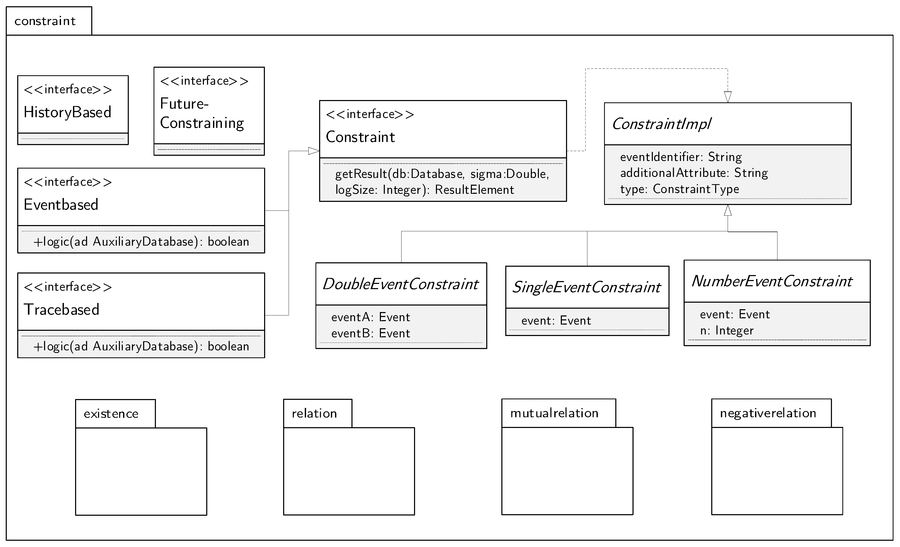
5.2.1. Package Model

The whole mining procedure does not operate on a plain XES file, but is using a customised POJO-model towards the needs of the JobRunner (see below). The omission of an XES loading module is a conscious decision reasoned within the flexibility and customisability of the library. The decision was made in favour of a simple EventLog class using a list of Traces holding a list of Events which again contains a list of Attributes. The latter is made of a key–value pair of Strings, e.g., (task, deliver). Mutator methods can be utilised for implementing loading modules but in some cases, loading duties can be transferred to third party frameworks (cf. Section 5.3).

In contrast to our work in [16], this implementation makes use of Java Objects instead of String representations of Events when emitting key–value pairs or for keys in HashMaps resulting in a additional performance boost (see Section 6).

5.2.2. JobRunner and Database as Centerpiece

The JobRunner is instantiated with an EventLog and a Configuration (package util). The former is described above and the latter contains: (i) a list (java.util.List<Class>) of constraints to consider; (ii) the ConstraintTypes to consider (i.e., ACTIVATION or TARGET); (iii) the event identifier (e.g., task); and (iv) the additional attribute (e.g., resource).

The mining job (see Algorithm 1) is launched with a call to job.run(). Java’s inbuilt Streaming-API cares for the parallel execution of the map- and reduce-function which forms a major foundation for utilising the main advantage of our approach: massive parallelism. The produced key–value pairs for the functions $\sigma$, $\eta$ and $ϵ$ are accumulated in an instance of the Database-class.

Algorithm 1: Setup of a mining job.

1 Configuration configuration = new Configuration();

2 configuration

3   .setEventIdentifier("task")

4   .setAdditionalAttribute("resource")

5   .addConstraint(Response.class)

6   .allConstraintTypes();

7 JobRunner job = new JobRunner(eventLog, configuration);

8 job.run();

9 job.getMiningResult();

The map-function (cf. Algorithm 2 for line numbers in round brackets) holds the nested for-loop as backbone (11, 13). Compared to our work in [16], the inner loop starts from 0 on, to comply with the full list of MP-Declare constraints.

Algorithm 2: The run and map functions.

1 publicvoid run() {

2   // MR-I: produce Key–Value Pairs

3   Database db = eventLog.getTraces().stream().map((trace) -> map(trace))

4      .reduce((accDb, currentDb) -> reduce(accDb, currentDb)).get();

5   // ’MR-II’: calculate Support and Confidence

6   mrii(db);

7 }

8 publicvoid map(Trace trace) {

9  Database database = new Database(configuration);

10  AuxilaryDatabase ad = new AuxilaryDatabase();

11  for (int i = 0; i < trace.getEvents().size(); i++) {

12   //…

13   for (int j = 0; j < trace.getEvents().size(); j++) {

14     for (Class<Constraint> c: getConfiguration().getConstraints()) {

15      Constraint impl = instantiate(c, events.get(i), events.get(j), -1,           ConstraintType.ACTIVATION);

16      if (impl instanceof Eventbased) {

17        Eventbased eventBasedImpl = (Eventbased) impl;

18        if (eventBasedImpl.logic(ad))

19         database.addSigma(eventBasedImpl, 1);

20        //…

21  //Tracebased-Constraints…

22 }

To support a high level of extendibility, the logic of each constraint template has moved from this global map-function and is now encapsulated for each specific template in a dedicated Java class (cf. Section 5.2.3). The nested for-loop simply iterates over the classes given in the Configuration-object (14) and calls the internal logic-function (18). The constraint template logic is completely executed in the responsible class, using an instance of util.AuxiliaryDatabase (10, 18) that provides the required data structures and meta-information like current values of the loop counters i and j.

MR-II is called before the function job.run() returns (Line 6) and delegates the support and confidence calculation to the constraint template classes, similar to MR-I. MR-II fills the MiningResult with ResultElements whose implementations are straightforward and, therefore, not described here in detail.

5.2.3. Package Constraint

As stated, an individual Java class is available for each constraint template. The library-inbuilt templates are spread over the sub-packages existence, relation, mutualrelation and negativerelation (cf. Figure 4). Each of them implements interfaces or extends abstract classes provided by the package constraint which describes the behaviour and structure of the templates.

For instance, the history based relation constraints (Precedence, AlternatePrecedence and ChainPrecedence) are implementing the interface HistoryBased. This is important to influence the control flow of the application such as the proper attribute filtering of events when constraints are instantiated (Line 15 in Algorithm 2):

HistoryBased constraints are activated with the second given event (eventB) and, therefore, eventB holds the additional condition in case of activation constraints, e.g., precedence(c, dx). FutureConstraining constraints work opposed to the former whilst having the additional attribute on the first given event (eventA), e.g., response(cy, d). The parameter eventA and eventB are available in relational constraints, as all of them extend the abstract class DoubleEventConstraint. The differentiation between Eventbased and Tracebased constraints is necessary, because Tracebased constraints are considered after the nested for-loop (Line 21 in Algorithm 2). In the following example, the internals of those constraint classes are illustrated by means of the Init constraint.

The init constraint simply cares about the first occurred event in a trace. Hence, only if the current position evaluates as 0, true is returned at Line 5 (Algorithm 3) and in turn the respective $\sigma$ value is adapted (Lines 18 and 19 in Algorithm 2). Instead of the position, the field first in the AuxiliaryDatabase could have been consulted in this case.

Algorithm 3: Class Init.

1 publicclassInitextendsSingleEventConstraintimplementsTracebased {

2   @Override

3   publicboolean logic(AuxilaryDatabase ad, int position, int size) {

4     if(position == 0)

5      return true;

6     else

7      return false;

8   }

9   @Override

10   publicResultElement getResult(Database db, double sigma, int logSize) {

11     returnnewResultElement(

12      this.getClass().toString(), getEvent(), sigma/logSize, 0.0d, this.getType());

13   }

14 }

The getResult method is called from MR-II and returns a ResultElement with the calculated support and confidence according to the formula defined in Section 4.2.

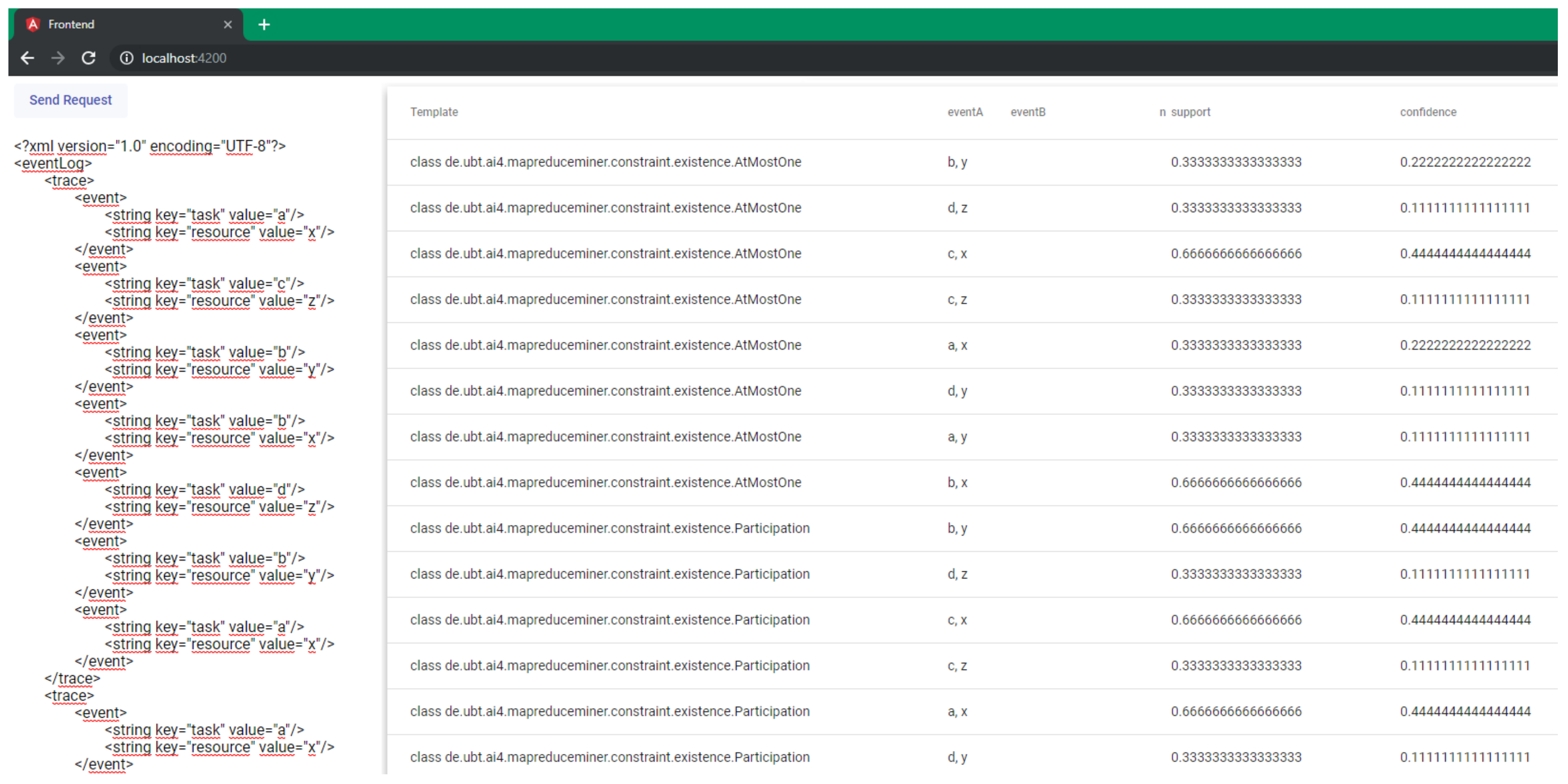
5.3. System Support

As stated, we refer to our GitHub-repository for detailed information about the MapReduce-Miner library as well as the implementing system described in this section. The respective projects are hosted there. For an overview of how to build the projects and how to use the library, we refer again to our Github-Repository. In this section, we show how to extend the mining procedure with custom constraint logic in view of the extensibility which addresses the full support covered in this paper.

The job (see Algorithm 1) is now configured using our custom constraint logic (config.addConstraint(WithinFiveSteps.class)) and a corresponding amended AuxiliaryDatabase (config.setAuxiliaryDatabaseClass(CustomAuxiliaryDatabase.class)). The custom logic is listed in Algorithm 4. The implementation resembles the Response class but uses an additional restriction that the task must not be more than five steps ahead (Line 7). In Line 5, the AuxiliaryDatabase is casted to our custom version, in order to obtain access to the required data structures on Lines 8 and 9.

Having finished the mining job, the MiningServiceResult containing the support and confidence values are returned and can be stored in a database or forwarded for further processing.

There is a Unit-test available in the library project, which attests the expected behaviour of our custom constraint: The test testCustomConstraintFulfill() operates on a trace

$$t_0=\langle (impl,x),(test,y),(test,y),(final-test,STE),(deliver,z)\rangle$$

and confirms that a discovered target constraint WithinFiveSteps(test, final-test ∧ final-test.resource = STE) holds the support value of 1. In contrast, the test testCustomConstraint() operates on a trace

$$t_1=\langle (impl,x),(test,y),(test,y),(test,y),(test,y),(test,y),(test,y),(final-test,STE),(deliver,z)\rangle$$

where the process gets stuck too long in the test loop (six events). Consequently, the target constraint WithinFiveSteps(test, final-test ∧ final-test.resource = STE) holds a support value less than 1.

Algorithm 4: Custom constraint WithinFiveSteps.

1 publicclassWithinFiveStepsextendsDoubleEventConstraint

2   implementsEventbased, FutureBased {

3     @Override

4    publicboolean logic(AuxiliaryDatabase ad) {

5      CustomAuxiliaryDatabase cad = (CustomAuxiliaryDatabase) ad;

6      if(cad.currentJ < cad.currentI+1) return false;

7      if(cad.currentJ > cad.currentI+5) return false;

8      if (!cad.tasksWithinFiveSteps.contains(super.getEventB())) {

9        cad.tasksWithinFiveSteps.add(super.getEventB());

10        return true;

11      } elsereturn false; }

12    }

13 }

Figure 5 shows an screenshot of the frontend project in the repository. The project contains a lightweight Angular 6 application tailored towards the chosen example. To address more process logs, representations and configurations, future generalisations of the architecture will be committed into the repository.

6. Evaluation

We present a comprehensive evaluation of our MapReduce-framework for the discovery of declarative process models including a quantitative performance comparison with related work. Additionally, we evaluate the resulting process models of different approaches in a qualitative way. In this section, three different real-life event logs are used: a Hospital Log [45], a Financial Log [46] and a Municipality Log [47].

6.1. Quantitative Performance Analysis

Comparison with Related Tools

Table 21. Performance evaluation with related tools.

	Single-Perspective *				Multi-Perspective **
	Financial Log		Hospital Log		Hospital Log
	-	-	-	-	Activation		Target
Approach	seq.	par.	seq.	par.	seq.	par.	seq.	par.
SQLMiner [14,15]	01:08	-	19:30	-	15:43	-	06:43:05	-
MINERful [11,12]	00:17	-	12:28	-	-	-	-	-
MapReduce	02:03	00:30	14:35	1:57	07:09	01:07	06:44	01:00

shows the results of our performance measurements compared to related work. The figures were measured on a Quad-Core i7 CPU @2.80 GHz. In this section, we describe the key findings. Based on the evaluation in [14,15], ${}^{*}$-superscripted figures include all relational constraints as well as NotSuccession and ${}^{**}$-superscripted figures include all history-based relational constraints.

Single-Perspective

MINERful is purely single-perspective and, in that case, MINERful performs better than MapReduce for both log files (17 s vs. 2 min and 12 min vs. 14 min, respectively), if MapReduce is executed sequentially. However, our approach is based on MapReduce and thus is designed for parallel execution. Having our approach running in parallel, it can compete with MINERful using the Financial Log (17 s vs. 30 s). Considering the challenging Hospital Log, MapReduce completes in less than 2 min and thus 10 times faster (SQLMiner) or 6 times faster (MINERful). The research papers presenting MINERful omit detailed implementation details, but we could not find any form of parallelism whilst scanning the code. Thus, we cannot compare this scenario. However, the supported level of parallelisation of MapReduce running on a cluster exceeds that of parallelising a conventional implementation such as MINERful anyway. Furthermore, as the parallelisation correlates with the performance (cf. Table 21 and [16]), we can raise the performance by just adding a new node to the cluster. As stated, the runtimes in Table 21 were measured on a Quad-Core CPU, which is tantamount to a cluster with just four nodes.

Multi-Perspective

Compared to MINERful, MapReduce is also capable of discovering multi-perspective constraints. To our knowledge, SQLMiner is the only other approach supporting MP-Declare discovery at the time of writing and thus the evaluation is grounded in a comparison with the SQLMiner here. The figures in Table 21 show the discovery of activation constraints as well as the discovery of target constraints. Where the SQLMiner shows an enormous difference between the two constraint types, the MapReduce approach shows constant runtimes reasoned in the computation method (see below). Considering activation constraints, MapReduce (in parallel) handles the Hospital Log in about 1 min compared to more than 15 min using the SQLMiner. Considering the target constraints, the computation with the SQLMiner takes several hours, whereas MapReduce finishes in 60 s (the runtime is less than in the single-perspective case, as less constraint templates are considered). The reason is that SQLMiner has to prepare the candidates (expensive JOIN operator on SQL tables), before evaluating the Support and Confidence, whereas MapReduce considers only valid constraints by default (nested for-loop).  

Analysis of different Log Files

Figure 6 shows performance measurements with two different log files, the Hospital Log (H) and the Municipality Log (M), during parallel execution with MapReduce. The figure holds values for Declare (SP) and MP-Declare (MP). We identify an expected increase of the duration when more constraint templates are considered (more constraint templates require more calculations) ranging from 8 to 49 s (M, SP) or from 60 to 325 s (H, MP). The runtimes for each constraint template remain constant, e.g., the duration for (M, MP) and 3 templates is 22 s (7.33 s per template on average) and for (M, MP) and 20 templates is 147 s (7.35 s on average).

We also can confirm that the Hospital Log is more challenging than the Municipality Log (13 s vs. 2.5 s per single-perspective template and 17 s vs. 7.5 s per multi-perspective template). The longer duration of multi-perspective constraints compared to single-perspective constraints is reasoned in the discovery of more constraints/information.

6.2. Qualitative Evaluation

For the qualitative evaluation, i.e., the comparison of the resulting process models of different approaches, we rather rely on a defined environment with a small, clean and synthetic log file, where we can count and recalculate the results by hand. This event log holds three traces:

$$t_0=\langle ax,cz,by,bx,dz,by,ax\rangle , t_1=\langle ax,bx,by,cx\rangle , t_2=\langle ay,cx,dy\rangle$$

In this section, we compare our MapReduce-approach with MINERful (single-perspective, cf.

Table 22. Discovered single-perspective Succession Constraints with MapReduce and MINERful.

		MapReduce		MINERful
Task A	Task B	Support	Confidence	Support	Confidence
a	a	0.25	0.083	-	-
a	b	0.778	0.518	0.778	0.518
a	c	0.85714	0.85714	0.85714	0.85714
a	d	0.66	0.44	0.66	0.44
b	a	0.44	0.296	0.44	0.296
b	b	0.6	0.3997	-	-
b	c	0.375	0.25	0.375	0.25
b	d	0.428571	0.142857	0.428571	0.285714
c	a	0.285714	0.285714	0.285714	0.285714
c	b	0.5	0.33	0.5	0.33
c	d	0.8	0.533	0.8	0.5334
d	a	0.33	0.22	0.33	0.22
d	b	0.285714	0.095238	0.285714	0.190476

) and with the SQLMiner (multi-perspective, cf.

Table 23. Discovered activational Response Constraints with MapReduce and SQLMiner.

			MapReduce		SQLMiner
Task A	Resource A	Task B	Support	Confidence	Support	Confidence
a	x	a	0.33	0.22	-	-
a	x	b	0.66	0.44	0.66	0.44
a	x	c	0.66	0.44	0.66	0.44
a	y	c	1.0	0.33	1.0	0.33
a	x	d	0.33	0.22	0.33	0.22
a	y	d	1.0	0.33	1.0	0.33
b	x	a	0.5	0.33	0.5	0.33
b	y	a	0.66	0.44	0.66	0.44
b	x	b	1.0	0.66	-	-
b	y	b	0.33	0.22	-	-
b	x	c	0.5	0.33	0.5	0.33
b	y	c	0.33	0.22	0.33	0.22
b	x	d	0.5	0.33	0.5	0.33
b	y	d	0.33	0.22	0.33	0.22
c	z	a	1.0	0.33	1.0	0.33
c	z	b	1.0	0.33	1.0	0.33
c	x	d	0.5	0.33	0.5	0.33
c	z	d	1.0	0.33	1.0	0.33
d	z	a	1.0	0.33	1.0	0.33
d	z	b	1.0	0.33	1.0	0.33

) with respect to the discovered process model.

Single-Perspective

Consider Table 22, which holds the results for the Succession-template. First, MINERful has not discovered constraints, where the tasks are equal (i.e., $Response(a,a)$ and $Response(b,b)$). However, we do not see any reason to neglect them, so we do include those constraints in the process model.

For some of the constraints, we detected discrepancies in the confidence values (highlighted with bold in Table 22). These occur because MINERful also calculates vacuously defined constraints. For instance, the confidence of the constraint $Succession(b,d)$ is calculated as $0.429·\frac{2}{3}=0.286$ in MINERful. The value 2 in the numerator is composed of the occurrence of events d and b in Trace $t_0$ and the non-occurrence of b in Trace $t_2$. Per definition, $Succession(b,d)$ is then vacuously fulfilled.

In contrast, the MapReduce-Miner considers only non-vacuously defined constraints. Therefore, the confidence value of $Succession(b,d)$ is calculated as $0.429·\frac{1}{3}=0.143$.

The same behaviour can be observed for the remaining constraint templates.

Multi-Perspective

The added value of MP-Declare compared to Declare is covered in the literature already (e.g., [15]). Using additional information in the mining procedure reveals deeper insights in the log, for instance that some constraints hold only if certain resources are involved.

Table 23 shows the discovered constraints using SQLMiner and MapReduce. The Activation Constraints matching the Response template are listed. Similar to MINERful on the single-perspective side, SQLMiner does not show constraints containing an equal event-identifier (the authors included the line "WHERE a.Task != b.Task" in the SQL-script). The rest of the discovered constraints is, besides rounding errors, consistent.

7. Conclusions

The presented approach is motivated by the fact that state-of-the-art declarative process mining tools do not support multiple perspectives at this moment. In particular, the discovery of constraints that impose additional statements on data values or ranges of data values, respectively, is an issue. We completed our work in [16], where we first addressed this research problem of discovering multi-perspective declarative process models by proposing an efficient mining framework for discovering MP-Declare models that leverage the latest big data analysis technology and build upon the distributed processing method MapReduce. We extended our previous work in several ways, inter alia, by introducing algorithms and descriptions for the full set of commonly accepted types of MP-Declare constraints. Furthermore, the conceptual architecture of our implemented prototype was reworked and improved such that new types of constraints can be easily defined and extracted by the user. The mining performance and effectiveness were tested with several real-life event logs. The experiments show that our technique solves this complex mining task in reasonable time.

The approach at hand represents a step into the direction of integrating process and data science and depicts a customisable and high performant declarative process mining technique. For future work, we plan to consider also correlation and time conditions. Furthermore, we will examine how to improve performance even more, for instance with alternative MapReduce frameworks that can be set up and tested with the proposed algorithms.

References

- Schönig, S.; Zeising, M.; Jablonski, S. Supporting collaborative work by learning process models and patterns from cases. In Proceedings of the 9th IEEE International Conference on Collaborative Computing: Networking, Applications and Worksharing, Austin, TX, USA, 20–23 October 2013; pp. 60–69. [Google Scholar]
- Van der Aalst, W. Process Mining: Discovery, Conformance and Enhancement of Business Processes; Springer: Berlin, Germany, 2011. [Google Scholar]
- Pichler, P.; Weber, B.; Zugal, S.; Pinggera, J.; Mendling, J.; Reijers, H.A. Imperative versus Declarative Process Modeling Languages: An Empirical Investigation. In Proceedings of the International Conference on Business Process Management, Clermont-Ferrand, France, 29 August–2 September 2011; pp. 383–394. [Google Scholar]
- Pesic, M.; Schonenberg, H.; van der Aalst, W.M.P. DECLARE: Full Support for Loosely-Structured Processes. In Proceedings of the 11th IEEE International Enterprise Distributed Object Computing Conference (EDOC 2007), Annapolis, MD, USA, 15–19 October 2007; pp. 287–300. [Google Scholar]
- Zeising, M.; Schönig, S.; Jablonski, S. Towards a Common Platform for the Support of Routine and Agile Business Processes. In Proceedings of the Collaborative Computing: Networking, Applications and Worksharing, Miami, FL, USA, 22–25 October 2014. [Google Scholar]
- De Leoni, M.; van der Aalst, W.M.P.; Dees, M. A general process mining framework for correlating, predicting and clustering dynamic behavior based on event logs. Inf. Syst. 2016, 56, 235–257. [Google Scholar] [CrossRef]
- Burattin, A.; Maggi, F.M.; Sperduti, A. Conformance Checking Based on Multi-Perspective Declarative Process Models. arXiv, 2015; arXiv:1503.04957. [Google Scholar] [CrossRef]
- Augusto, A.; Conforti, R.; Dumas, M.; La Rosa, M.; Maggi, F.M.; Marrella, A.; Mecella, M.; Soo, A. Automated Discovery of Process Models from Event Logs: Review and Benchmark. CoRR 2017, arXiv:1705.02288. [Google Scholar] [CrossRef]
- Van der Aalst, W.M.P. Process Mining—Data Science in Action, 2nd ed.; Springer: Berlin, Germany, 2016. [Google Scholar]
- Leemans, S.J.J.; Fahland, D.; van der Aalst, W.M.P. Scalable process discovery and conformance checking. Softw. Syst. Model. 2018, 17, 599–631. [Google Scholar] [CrossRef] [PubMed]
- Di Ciccio, C.; Mecella, M. A Two-Step Fast Algorithm for the Automated Discovery of Declarative Workflows. In Proceedings of the 2013 IEEE Symposium on Computational Intelligence and Data Mining (CIDM), Singapore, 16–19 April 2013; pp. 135–142. [Google Scholar]
- Di Ciccio, C.; Mecella, M. On the Discovery of Declarative Control Flows for Artful Processes. ACM TMIS 2015, 5, 1–37. [Google Scholar] [CrossRef]
- Maggi, F.M. Declarative Process Mining with the Declare Component of ProM. In Proceedings of the Business Process Management Demos, Beijing, China, 26–30 August 2013. [Google Scholar]
- Schönig, S.; Rogge-Solti, A.; Cabanillas, C.; Jablonski, S.; Mendling, J. Efficient and Customisable Declarative Process Mining with SQL. In Proceedings of the International Conference on Advanced Information Systems Engineering, Tallinn, Estonia, 11–15 June 2016. [Google Scholar]
- Schönig, S.; Di Ciccio, C.; Maggi, F.M.; Mendling, J. Discovery of Multi-perspective Declarative Process Models. In Proceedings of the International Conference on Service-Oriented Computing, Hangzhou, China, 12–15 November 2016; pp. 87–103. [Google Scholar]
- Sturm, C.; Schönig, S.; Jablonski, S. A MapReduce Approach for Mining Multi-Perspective Declarative Process Models. In Proceedings of the 20th International Conference on Enterprise Information Systems, ICEIS 2018, Funchal, Portugal, 21–24 March 2018; pp. 585–595. [Google Scholar]
- Maggi, F.M.; Mooij, A.; van der Aalst, W. User-Guided Discovery of Declarative Process Models. In Proceedings of the 2011 IEEE Symposium on Computational Intelligence and Data Mining (CIDM), Paris, France, 11–15 April 2011; pp. 192–199. [Google Scholar]
- Di Ciccio, C.; Schouten, M.H.M.; de Leoni, M.; Mendling, J. Declarative Process Discovery with MINERful in ProM. In Proceedings of the Business Process Management Demos, Innsbruck, Austria, 31 August–3 September 2015; pp. 60–64. [Google Scholar]
- Westergaard, M.; Stahl, C.; Reijers, H. UnconstrainedMiner: Efficient Discovery of Generalized Declarative Process Models; BPM CR, No. BPM-13-28; BPM Center: Eindhoven, The Netherlands, 2013. [Google Scholar]
- Maggi, F.; Bose, R.; van der Aalst, W. A Knowledge-Based Integrated Approach for Discovering and Repairing Declare Maps. In Proceedings of the International Conference on Advanced Information Systems Engineering, Tallinn, Estonia, 11–15 June 2013. [Google Scholar]
- Di Ciccio, C.; Maggi, F.M.; Montali, M.; Mendling, J. Ensuring Model Consistency in Declarative Process Discovery. In Proceedings of the International Conference on Business Process Management, Innsbruck, Australia, 31 August–3 September 2015; pp. 144–159. [Google Scholar]
- Di Ciccio, C.; Maggi, F.M.; Montali, M.; Mendling, J. Resolving inconsistencies and redundancies in declarative process models. Inf. Syst. 2017, 64, 425–446. [Google Scholar] [CrossRef] [Green Version]
- Bose, J.C.; Maggi, F.M.; van der Aalst, W. Enhancing Declare Maps Based on Event Correlations. In Proceedings of the Business Process Management, Beijing, China, 26–30 August 2013; pp. 97–112. [Google Scholar]
- Vanden Broucke, S.K.L.M.; Vanthienen, J.; Baesens, B. Declarative process discovery with evolutionary computing. In Proceedings of the 2014 IEEE Congress on Evolutionary Computation (CEC), Beijing, China, 6–11 July 2014; pp. 2412–2419. [Google Scholar] [CrossRef]
- Lamma, E.; Mello, P.; Montali, M.; Riguzzi, F.; Storari, S. Inducing Declarative Logic-Based Models from Labeled Traces. In Proceedings of the International Conference on Business Process Management, Brisbane, Australia, 24–28 September 2007; pp. 344–359. [Google Scholar]
- Chesani, F.; Lamma, E.; Mello, P.; Montali, M.; Riguzzi, F.; Storari, S. Exploiting Inductive Logic Programming Techniques for Declarative Process Mining. Trans. Petri Nets Other Models Concurrency 2009, 2, 278–295. [Google Scholar]
- Räim, M.; Di Ciccio, C.; Maggi, F.M.; Mecella, M.; Mendling, J. Log-Based Understanding of Business Processes through Temporal Logic Query Checking. In Proceedings of the OTM Confederated International Conferences “On the Move to Meaningful Internet Systems”, Amantea, Italy, 27–31 October 2014; pp. 75–92. [Google Scholar]
- Westergaard, M.; Maggi, F.M. Looking into the Future: Using Timed Automata to Provide A Priori Advice about Timed Declarative Process Models; OTM; LNCS; Springer: Berlin, Germany, 2012; Volume 7565, pp. 250–267. [Google Scholar]
- Maggi, F.M. Discovering Metric Temporal Business Constraints from Event Logs. In Proceedings of the International Conference on Business Informatics Research, Lund, Sweden, 22–24 September 2014; pp. 261–275. [Google Scholar]
- Schönig, S.; Cabanillas, C.; Jablonski, S.; Mendling, J. A Framework for Efficiently Mining the Organisational Perspective of Business Processes. Decis. Support Syst. 2016, 89, 87–97. [Google Scholar] [CrossRef]
- Cabanillas, C.; Schönig, S.; Sturm, C.; Mendling, J. Mining Expressive and Executable Resource-Aware Imperative Process Models. In Proceedings of the International Conference on Enterprise, Business-Process and Information Systems Modeling, Tallinn, Estonia, 11–12 June 2018; pp. 3–18. [Google Scholar]
- Schönig, S.; Cabanillas, C.; Ciccio, C.D.; Jablonski, S.; Mendling, J. Mining team compositions for collaborative work in business processes. Softw. Syst. Model. 2018, 17, 675–693. [Google Scholar] [CrossRef]
- Montali, M.; Chesani, F.; Mello, P.; Maggi, F.M. Towards data-aware constraints in declare. In Proceedings of the 28th Annual ACM Symposium on Applied Computing, Coimbra, Portugal, 18–22 March 2013; pp. 1391–1396. [Google Scholar]
- Maggi, F.M.; Dumas, M.; García-Bañuelos, L.; Montali, M. Discovering Data-Aware Declarative Process Models from Event Logs. In Proceedings of the Business Process Management 2013, Beijing, China, 26–30 August 2013; pp. 81–96. [Google Scholar] [CrossRef]
- Burattin, A.; Maggi, F.M.; Sperduti, A. Conformance checking based on multi-perspective declarative process models. Expert Syst. Appl. 2016, 65, 194–211. [Google Scholar] [CrossRef] [Green Version]
- Ackermann, L.; Schönig, S.; Jablonski, S. Simulation of Multi-perspective Declarative Process Models. In Proceedings of the Business Process Management Workshops—BPM 2016 International Workshops, Rio de Janeiro, Brazil, 19 September 2016; Revised Papers. pp. 61–73. [Google Scholar]
- Ackermann, L.; Schönig, S.; Petter, S.; Schützenmeier, N.; Jablonski, S. Execution of Multi-perspective Declarative Process Models. On the Move to Meaningful Internet Systems. In Proceedings of the OTM 2018 Conferences—Confederated International Conferences: CoopIS, C&TC, and ODBASE 2018, Valletta, Malta, 22–26 October 2018; pp. 154–172. [Google Scholar]
- Sturm, C.; Schönig, S.; Ciccio, C.D. Distributed Multi-Perspective Declare Discovery. In Proceedings of the BPM Workshops, Barcelona, Spain, 10–15 September 2017. [Google Scholar]
- Van der Aalst, W.; Pesic, M.; Schonenberg, H. Declarative Workflows: Balancing Between Flexibility and Support. Comput. Sci. Res. Dev. 2009, 23, 99–113. [Google Scholar] [CrossRef]
- Montali, M.; Pesic, M.; van der Aalst, W.M.P.; Chesani, F.; Mello, P.; Storari, S. Declarative Specification and Verification of Service Choreographies. ACM Trans. Web 2010, 4, 3. [Google Scholar] [CrossRef]
- Burattin, A.; Maggi, F.M.; van der Aalst, W.M.; Sperduti, A. Techniques for a Posteriori Analysis of Declarative Processes. In Proceedings of the 16th IEEE International Enterprise Distributed Object Computing Conference, EDOC 2012, Beijing, China, 10–14 September 2012; pp. 41–50. [Google Scholar]
- Dean, J.; Ghemawat, S. MapReduce: Simplified Data Processing on Large Clusters. Commun. ACM 2008, 51. [Google Scholar] [CrossRef]
- Foundation, A.S. Apache Hadoop. 2006. Available online: https://hadoop.apache.org/ (accessed on 5 January 2019).
- Wu, D.; Sakr, S.; Zhu, L. Big Data Programming Models. In Handbook of Big Data Technologies; Zomaya, A.Y., Sakr, S., Eds.; Springer International Publishing: Berlin, Germany, 2017; pp. 31–63. [Google Scholar]
- Boudewijn van Dongen, Real-Life Event Logs—Hospital Log. 2011. Available online: https://doi.org/10.4121/uuid:d9769f3d-0ab0-4fb8-803b-0d1120ffcf54 (accessed on 14 January 2019).
- Boudewijn van Dongen, BPI Challenge 2017. Available online: https://doi.org/10.4121/uuid:5f3067df-f10b-45da-b98b-86ae4c7a310b (accessed on 14 January 2019).
- Boudewijn van Dongen, BPI Challenge 2015. Available online: https://doi.org/10.4121/uuid:31a308ef-c844-48da-948c-305d167a0ec1 (accessed on 14 January 2019).