Glomerular Filtration Rate Estimation by a Novel Numerical Binning-Less Isotonic Statistical Bivariate Numerical Modeling Method

Abstract

Statistical bivariate numerical modeling is a method to infer an empirical relationship between unpaired sets of data based on statistical distributions matching. In the present paper, a novel efficient numerical algorithm is proposed to perform bivariate numerical modeling. The algorithm is then applied to correlate glomerular filtration rate to serum creatinine concentration. Glomerular filtration rate is adopted in clinical nephrology as an indicator of kidney function and is relevant for assessing progression of renal disease. As direct measurement of glomerular filtration rate is highly impractical, there is considerable interest in developing numerical algorithms to estimate glomerular filtration rate from parameters which are easier to obtain, such as demographic and ‘bedside’ assays data.

1. Introduction

Several real-world complex phenomena in virtually any branch of science lack accurate mathematical descriptions. In these cases, predicting the value of a variable by any analytically derived expression is not viable, therefore, empirical or statistical methods are generally exploited to develop a model of the observed phenomenon. Examples are found in seismic facies visualization and interpretation [1], cell-free protein synthesis [2], in marine stratigraphy [3], and in electrical load forecasting [4].

The complex phenomenon that triggered the present research is the estimation of glomerular filtration rate (GFR) in the context of eHealth. Estimated glomerular filtration rate is a common test to measure a patient’s level of kidney function and to determine a stage of kidney disease in case of renal malfunction. Results of GFR estimation are measured in milliliter per minute per squared meter (mL/min/m²) as GFR is related, in fact, to a flow rate per area-unit through the filtering structures that constitute the kidneys, called glomeruli. Each glomerulus is a network of capillaries, located at the beginning of a nephron in the kidney. The blood is filtered across the capillary walls through the glomerular filtration barrier. The filtrate then enters the renal tubule of the nephron. If the GFR is low, the kidneys are not working as well as they should. Estimated GFR tells doctors the stage of kidney disease and helps medical team on planning a treatment. Glomerular filtration rate is also frequently required for evaluating optimal dosage for medications [5,6].

Determination of true GFR is time-consuming, costly and difficult to perform [7,8]. Thus, there is considerable interest in developing models to estimate GFR using simpler parameters such as a patient’s age, weight, height, gender and values which can be more conveniently measured as part of a standard blood test. Modern instrumentation would also afford quick and reliable bedside testing. (Bedside testing, also referred to as point-of-care testing, indicates a performance of clinical laboratory testing at the site of patient care rather than in a laboratory.) as an instance of eHealth applications [9]. A simple, yet reliable, way to estimate a patient’s glomerular filtration rate is by creatinine test. Creatinine is a chemical waste produced by muscle metabolism and, to a smaller extent, by meat intake. Healthy kidneys filter creatinine and other waste products from blood and the body disposes of the filtered waste products via urination. If kidneys are not functioning properly, an increased level of creatinine may accumulate in the blood flow. A serum creatinine test measures the level of creatinine in the blood and provides an estimation of how well the kidneys filter. Results of the creatinine blood test are measured in milligrams per deciliter (mg/dL). The normal range for creatinine in the blood can vary from lab to lab, between men and women, by ethnicity and by age. Since the amount of creatinine in the blood increases with muscle mass, men usually exhibit higher creatinine levels than women. Generally, a high serum creatinine level indicates that kidneys are not filtering properly, although creatinine level may temporarily increase in case of dehydration, low blood volume, large amount of meat intake or if a patient is subject to certain medications. Dietarily supplemented creatinine may result in increased creatinine levels.

Numerical data modeling helps in finding an empirical relationship between serum creatinine and glomerular filtration rate on the basis of a set of measured data-pairs. The most common set of tools used to infer a relationship between variables is known under the encompassing name of numerical modeling (see, e.g., [10,11]). Traditional forms of data modeling are based on some parametrised function whose graph is made to lay reasonably close to the points making up the experimental dataset. Values for the parameters are typically calculated using the least squares method [12]. Numerical data modeling is a broad research area which involves a wide variety of novel artificial-intelligence and statistical tools. A few examples of recent contributions in this field are Petri nets to model honeypot [13], extreme learning machines in monthly precipitation time series forecasting [14], and recurrent neural networks to language modeling, emotion classification and polyphonic modeling [15]. Specifically to the problem treated in this paper, traditional artificial neural-network techniques to build up empirical models of GFR were proposed and tested in the scientific literature, although their performance appeared unsatisfactory or questionable [16,17]. A general observation about machine learning techniques is that they are characterized by non-negligible computational burden and computation times, which may be unpractical to implement in inexpensive devices conceived for real-time data processing.

Examining the empirical relationship between serum creatinine concentration and glomerular filtration rate, it is immediate to realize that their dependence is of monotonically decreasing nature, namely, an increased level of serum creatinine corresponds to a reduced value of filtration rate. This observation suggests that, rather than generic data modeling, it is appropriate to call for a specific class known as isotonic modeling. Isotonic data modeling allows greater freedom for the model to fit data by constructing a piecewise linear function, described by a lookup table (LUT). Overfitting is avoided by requiring the function to be isotonic, which is reasonable whenever the underlying physical phenomenon is inherently monotonic (such as the relationship between percentage body fat and waist circumference [18]). The specialized literature offers a number of algorithms to determine the LUT values-entries that satisfy a least-squares condition [19,20].

Statistical bivariate data modeling (SBR) provides an improvement over isotonic modeling. Its advantages derive from the fact that it relies on inferring the relationship between the statistical distributions of the variables, rather than on the values of the variables. SBR is not based on a least squares method, therefore, it does not require data to be associated in ordered pairs. This makes it ideal for correlating two quantities that cannot be both measured on the same individual. The algorithm presented in [21] independently estimates the probability density functions (PDF) of the two variables by dividing the dataset ranges into bins and by populating look-up tables with the relative frequencies of occurrence. The PDFs are then integrated numerically to obtain the cumulative distribution functions (CDF) which are, or can be licitly adjusted to be, bijective and allow for the numerical model to be obtained as a map between values with equal probabilities.

This paper proposes a novel algorithm developed to make statistical bivariate numerical modeling more versatile and faster over large datasets by entirely avoiding the binning (previously required to estimated PDFs) and numerical integration operations (previously required to estimated a CDF from a PDF that it is associated to). The main focuses of the present paper are:

• developing a computationally simple and light modeling algorithm that can be easily implemented on a portable, inexpensive hardware, which will aid bedside testing; since bedside testing produces new data all the time, a desirable feature of the modeling algorithm would be the ability to incorporate new data as they become available;
• applying the modeling algorithm to a specific problem, namely quick and reliable renal function assessment by creatinine assay data, both for pedriatic and adult patients.

The present paper is organized as follows. Section 2 recalls the notion of bivariate statistical modeling and explains the main idea and the details about the proposed binning-less bivariate statistical modeling algorithm. Section 2 also illustrates a comparison of features of the proposed statistical modeling algorithm with three machine-learning algorithms (Multi-layer perceptron, support vector regression and random trees) on a benchmark problem. Section 3 explains an analysis of the glomerular-filtration-rate (GFR) estimation based on creatinine levels and illustrates such analysis by means of numerical tests performed on a dataset drawn from a study on pediatric patients in mainland China as well as on a dataset about adult patients. Section 4 concludes the paper. Computer codes to implement the modeling algorithm described in the paper are reported in the Appendix A.

2. Binning-Less Statistical Bivariate Numerical Modeling Algorithm

Given random variables X and Y, for which we expect the existence of a monotonic function f such that $Y=f\left(X\right)$, let $D_X\in {\mathbb{R}}^n$ and $D_Y\in {\mathbb{R}}^m$ be arrays whose components are realizations of X and Y respectively. The developed numerical modeling algorithm is encapsulated in a function that takes the $D_X$ and $D_Y$ dataset arrays along with an $x\in [x_{\min },x_{\max }]$ for which the estimated value of $f\left(x\right)$ is returned.

Denoting by $P_X\left(x\right)$ and by $P_Y\left(y\right)$ the respective CDFs of X and Y, we recall from the second author’s previous contributions [21,22] that

$$f\left(x\right)=\left\{\begin{array}{cc}{P}_Y^{-1}\left(P_X\left(x\right)\right)\hfill & \mathrm{if}f\mathrm{is}\mathrm{monotonically}\mathrm{increasing},\hfill \\ P_Y^{-1}(1-P_X\left(x\right))\hfill & \mathrm{if}f\mathrm{is}\mathrm{monotonically}\mathrm{decreasing}.\hfill \end{array}\right.$$

(1)

The proposed SBR-type numerical modeling procedure can be separated into two parts: the evaluation of a cumulative distribution function and the evaluation of an inverse cumulative distribution function. Details of the proposed method are outlined in the Section 2.1, while the Section 2.2 is devoted to a comparison between the proposed methods and state-of-the-art machine-learning techniques. (In the machine-learning jargon, the estimation of the cumulative distribution functions is equivalent to a ‘learning’ phase, while the application of the relationship (1) is equivalent to a ‘forward’ phase.)

2.1. Proposed Numerical Solutions

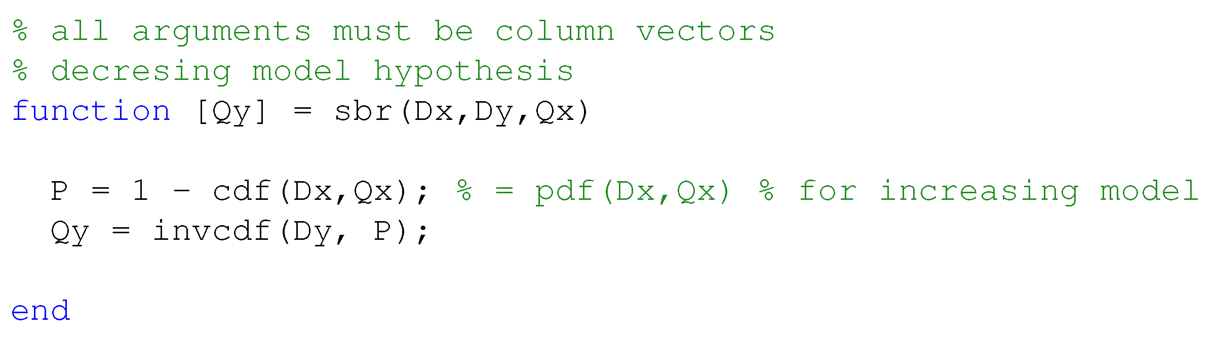
The evaluation of cumulative distributions is handled by the cdf function defined in Algorithm 1, while the evaluation of an inverse cumulative distribution is handled by invCdf function defined in Algorithm 2. Besides the argument for the CDF (or inverse CDF), both procedures require a dataset from which to infer the actual distributions. Algorithm 3 provides a pseudocode for joining the two parts together, according to (1), in the case that a monotonically increasing model is sought. If the model is expected to be monotonically decreasing, then the value P on Line 3 should be replaced by its complement $1-P$.

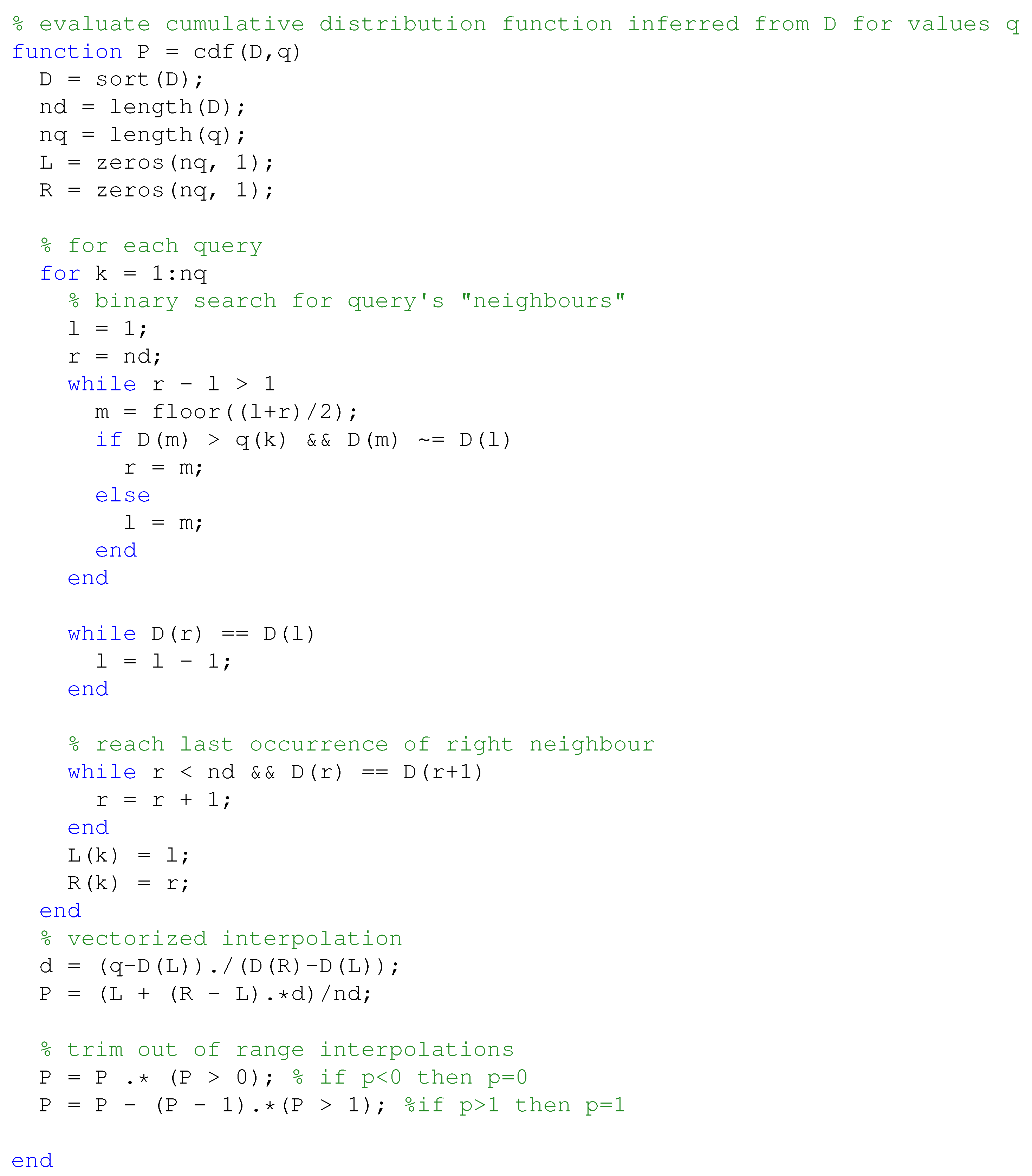
We developed a binning-less procedure to estimate the value of the CDF $P\left(q\right)$ of a generic random variable Q for which n realizations are stored as the components of an array D. The main idea to avoid binning is to estimate the cumulative distribution function of a dataset without resorting to an estimation of the probability density function first. Such result can be achieved by embracing the definition of CDF itself, which leads us to counting the number of realizations whose values are smaller than (or equal to) q and dividing this count by n. The solution shown in Algorithm 1 expands this idea to allow for a continuous, strictly monotonic interpolation for values that are not included in the original dataset. (Array indexing is 1-based and symbol ∧ denotes logical conjunction.)

Algorithm 1 Cumulative distribution function estimation

1: functioncdf(D, q) 2:     $D\leftarrow$ sort $\left(D\right)$            ▹ Dataset is sorted in ascending order 3:     $n\leftarrow$ length $\left(D\right)$           ▹ Gets the cardinality of the dataset D 4:     $l\leftarrow 1$ 5:     $r\leftarrow n$ 6:     while $r-l>1$ do 7:         $m\leftarrow ⌊(l+r)/2⌋$ 8:         if $D\left[m\right]>q\wedge D\left[m\right]\ne D\left[l\right]$ then 9:            $r\leftarrow m$ 10:         else 11:            $l\leftarrow m$ 12:     while $D\left[r\right]=D\left[l\right]$ do 13:         $l\leftarrow l-1$ 14:     while $r<n\wedge D\left[r\right]=D[r+1]$ do 15:         $r\leftarrow r+1$ 16:     $d\leftarrow (q-D[l\left]\right)/\left(D\right[r]-D[l\left]\right)$ 17:     $P\leftarrow (l+d·(r-l\left)\right)/n$ 18:     if $P<0$then            ▹ Trimming out-of-range interpolations 19:         $P\leftarrow 0$ 20:     else if $P>1$ then 21:         $P\leftarrow 1$ 22:     return P

Here are a few comments about Algorithm 1:

• Line 2: The algorithm is notably simplified by sorting the entries of D in ascending order.
• Lines 4–13: This part is essentially a binary search for q in array D. The loop starts with indexes l and r as the endpoints of D and ends with l as the index of the last value less than q, and r as that of the first value greater than q. The only exception that may occur is handled in lines 14–16.
• Line 8: Making sure that $D\left[m\right]\ne D\left[l\right]$ is needed to prevent l and r from converging to 1 and 2 respectively, in the case that q is smaller than all elements in D.
• Lines 14–16: This loop is needed to fix l in the case that it converges to $n-1$ as a consequence of q being greater than all values in D.
• Lines 17–19: The previous operations already guarantee that l is the last index for the value $D\left[l\right]$, which means that there are l elements in D which are less than or equal to $D\left[l\right]$. This loop finds r, the count of elements whose values are smaller than (or equal to) the value $D\left[r\right]$.
• Lines 20–21: The probability $P\left(D\right[l\left]\right)$ is estimated by the ratio $l/n$, whilst the probability $P\left(D\right[r\left]\right)$ is estimated by the ratio $r/n$. The sought probability $P\left(q\right)$ is obtained via linear interpolation of the two.
• Lines 22–26: These checks fix the CDF for values of the query point q that lay outside the range of D.

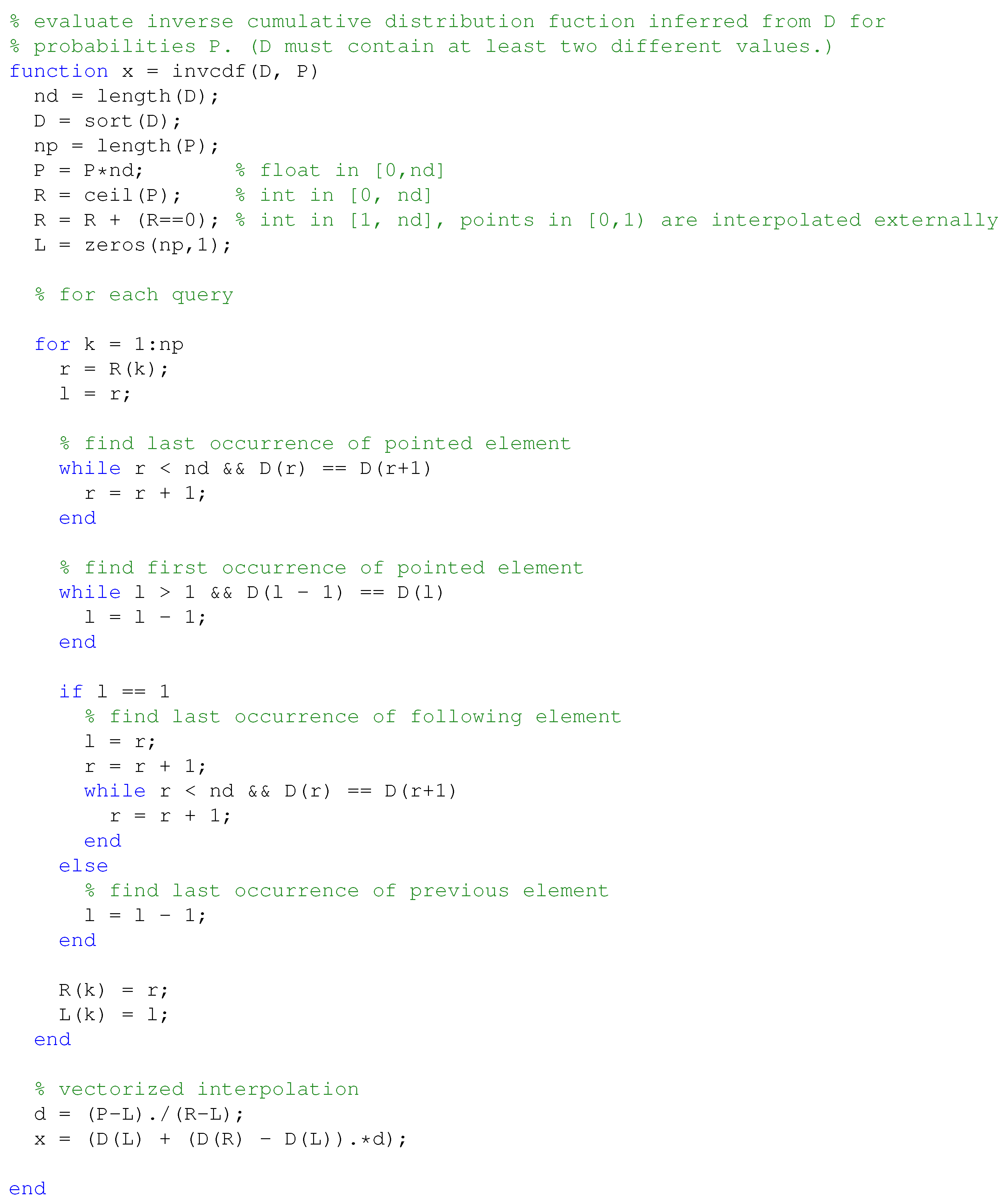
The evaluation of the inverse CDF is based on the same principle applied in a reverse fashion: the input argument is a probability, it is multiplied by the cardinality n of the dataset D and the result of such multiplication is rounded to an integer r. If the dataset D is sorted, then there will be r values less than or equal to $D\left[r\right]$. The Algorithm 2 again allows for a continuous, strictly monotonic interpolation to yield values that are not included in the original dataset.

Algorithm 2 Inverse cumulative distribution function estimation

1: functioninvCdf (D, $P_q$) 2:     $D\leftarrow$ sort $\left(D\right)$ 3:     $n\leftarrow$ length $\left(D\right)$ 4:     $p\leftarrow P_q·n$ 5:     $r\leftarrow ⌈p⌉$ 6:     if $r=0$ then 7:         $r\leftarrow 1$ 8:     $l\leftarrow r$ 9:     while $r<n\wedge D\left[r\right]=D[r+1]$ do 10:         $r\leftarrow r+1$ 11:     while $l>1\wedge D[l-1]=D\left[l\right]$ do 12:         $l\leftarrow l-1$ 13:     if $l=1$ then 14:         $l\leftarrow r$ 15:         $r\leftarrow r+1$ 16:         while $r<n\wedge D\left[r\right]=D[r+1]$ do 17:            $r\leftarrow r+1$ 18:     else 19:         $l\leftarrow l-1$ 20:     $d\leftarrow (p-l)/(r-l)$ 21:     $q\leftarrow D\left[l\right]+d·\left(D\right[r]-D[l\left]\right)$ 22:     return q

Here are a few comments about Algorithm 2:

• Line 2: The algorithm is notably simplified by sorting D in ascending order.
• Line 4: The input probability is denormalized into the range $[0,n]$.
• Lines 5–9: The indexes r and l take the value of p rounded to the next integer to be used as an index, which also requires r and l to be non-zero.
• Lines 10–12: The index r is made to point to the last occurrence of the smallest value whose CDF is greater than the query probability.
• Lines 13–15, 20: l is made to point to the first occurrence of the same value.
• Line 23: Normally l is then made to point to the previous element which is the last occurrence of the greatest value whose CDF is less than the query probability.
• Lines 16–21: If l is already pointing to the first value of the array then l takes the value of r and r is made to point to the last occurrence of the following value.
• Lines 25–26: The inverse cumulative distribution function value $P^{-1}(l/n)$ is estimated by $D\left[l\right]$, whilst the inverse cumulative distribution function value $P^{-1}(r/n)$ is estimated by $D\left[r\right]$. Nearby values are obtained via linear interpolation.

Algorithm 3 Statistical Bivariate Numerical Modeling (for monotonically increasing models)

1: functionstatisticalModeling ($D_X$, $D_Y$, $x_q$) 2:     $P\leftarrow$ cdf $(D_X,x_q)$             ▹ Evaluate CDF for value $x_q$ in dataset $D_X$ 3:     $y_q\leftarrow$ invCdf $(D_Y,P)$        ▹ Evaluate inverse CDF for probability P on dataset $D_Y$ 4:     return $y_q$

In the Algorithm 3, $D_X$ and $D_Y$ denote again the x-component and the y-components of the dataset to be modeled, while the quantity $x_q$ denotes a query value, not belonging to the set $D_X$ but laying within the same range values. The Algorithm 3 estimates the value of the model $f\left(x_q\right)$ and returns such estimate as $y_q$. Most typically, the query values are chosen equally spaced within the range-interval $[x_{\min },x_{\max }]$.

MATLAB codes to implement the three functions described in the present section are reported in the Appendix A.

Ideally, it should hold that invCdf(cdf$\left(q\right))=q$. To verify this identity, we ran a numerical test on the Algorithms 1 and 2 using the real-world dataset analyzed in Section 3.2. For each element q in the array, we calculated the relative deviation from identity

$$\delta =\left|\frac{\mathrm{INV}\mathrm{C}\mathrm{DF}(\mathrm{CDF}(q))-q}{q}\right|.$$

(2)

The largest value of $\delta$ was found to be in the order of ${10}^{-15}$, which is definitely acceptable.

Example 1.

To conclude this section of the paper, let us consider a minimal working numerical example. Let$D_X=[2,3,5,5,6,6,7,9]$and$D_Y=[6,7,10,10,11,11,11,12,15,20]$, i.e.,$n=8$,$m=10$. The actual underlying model is$f\left(x\right)=2x+2$. Note that the data are not paired. Both arrays are already sorted for simplicity. Let the query point be$x_q=4$: we expect the result of statistical numerical modeling (Algorithm 3) to be$y_q\approx 10$. The proposed procedure prescribes first to estimate the probability$P_X\left(4\right)$: the Algorithm 1 will find$l=2$and$r=4$. The Algorithm 1 then will compute the linear interpolation:

$$d=\frac{x_q-X\left[l\right]}{X\left[r\right]-X\left[l\right]}=\frac{4-3}{5-3}=0.5\Rightarrow P_X\left(4\right)=\frac{l+d·(r-l)}{n}=\frac{2+0.5·(4-2)}{8}=0.375.$$

The proposed procedure prescribes next to estimate the inverse probability$P_Y^{-1}\left(0.375\right)$: the Algorithm 2 will find$p=0.375·m=3.75$,$r=4$and$l=2$. By linear interpolation, the Algorithm 2 then finds

$$d=\frac{p-l}{r-l}=\frac{3.75-2}{4-2}=0.875\Rightarrow P_Y^{-1}\left(0.375\right)=D\left[l\right]+d·(D\left[r\right]-D\left[l\right])=7+0.875·(10-7)=9.625,$$

which is remarkably close to the exact value 10, given the extremely limited number of available data-samples.

2.2. Comparison with Machine-Learning Techniques

The present contribution developed an algorithm for estimating the CDF without using binning. When discretization (like binning) is required, machine learning algorithms are often utilized. These may include artificial neural networks (ANN) [23], support vector regression (SVR) [24] and regression trees/forests (RT) [25], that help creating an empirical model that outputs the prediction value, mitigating outliers and trying to reduce overfitting. These artificial intelligence techniques, however, are known to be computationally expensive and time consuming because they need extensive training.

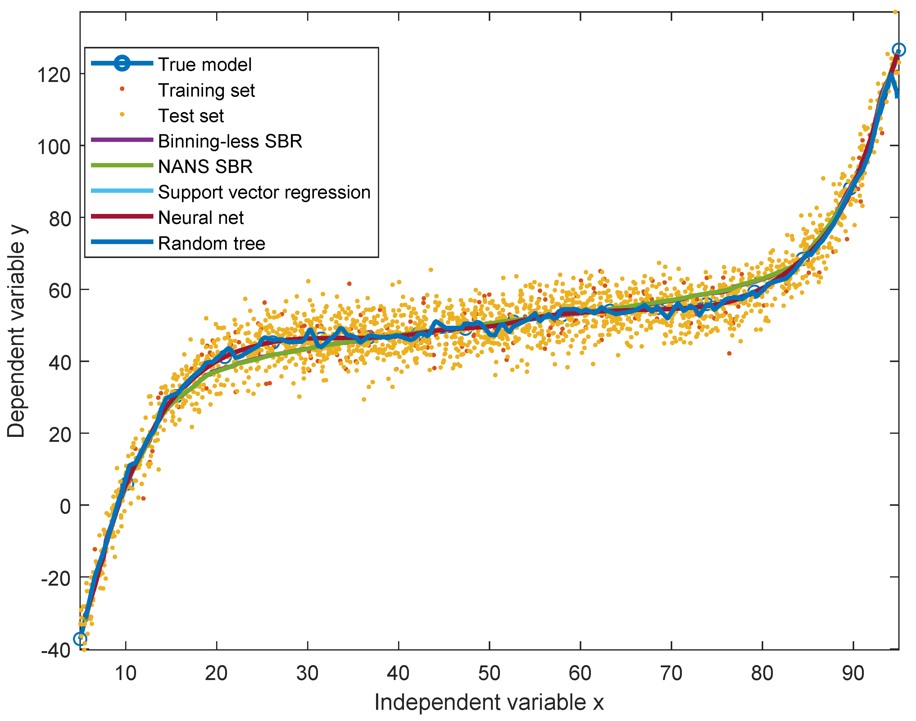
In order to test the effectiveness and time-efficiency of the proposed non-linear modeling technique against machine-learning algorithms, we effected a preliminary experiment on a toy problem, namely, on modeling synthetic data obtained by adding noise to a monotonic fifth-order polynomial. The machine-learning techniques adopted for comparison are ANN (a 1-10-1 multi-layer perceptron), SVR (with Gaussian kernel functions) and RT. In order to compare objectively the results of modeling, we adopted the following figures drawn from the scientific literature: mean squared error (MSE), mean absolute error (MAE), variance-accounted-for (VAF) and coefficient of correlation ($\rho$). For a generic prediction-making system, represented by the function $f\left(x\right)$, being validated over the set of data points $\{(x_1,y_1),(x_2,y_2),\dots ,(x_n,y_n)\}$, these indexes are defined as

$$\begin{array}{c}\mathit{MSE}=\frac{1}{n}\sum _{i=1}^n{(f\left(x_i\right)-y_i)}^2,\hfill \end{array}$$

(3)

$$\begin{array}{c}\mathit{MAE}=\frac{1}{n}\sum _{i=1}^n|f\left(x_i\right)-y_i|,\hfill \end{array}$$

(4)

$$\begin{array}{c}\rho =\frac{{\sum }_{i=1}^n(f\left(x_i\right)-\overline{f})(y_i-\overline{y})}{\sqrt{{\sum }_{i=1}^n{(f\left(x_i\right)-\overline{f})}^2{\sum }_{i=1}^n{(y_i-\overline{y})}^2}},\hfill \end{array}$$

(5)

$$\begin{array}{c}\mathit{VAF}=\left(1-\frac{{\sum }_{i=1}^n{(f\left(x_i\right)-\overline{f}-(y_i-\overline{y}))}^2}{{\sum }_{i=1}^n{(y_i-\overline{y})}^2}\right)·100\%,\hfill \end{array}$$

(6)

where $\overline{y}=\frac{1}{n}{\sum }_{i=1}^n{y}_i$ and $\overline{f}=\frac{1}{n}{\sum }_{i=1}^{n}f\left(x_i\right)$. The coefficient of correlation $\rho$ takes values in the interval $[-1,1]$. If variables are directly correlated, then we expect the coefficient to approach $+1$ while, if variables are inversely correlated, we expect a value of the coefficient of correlation close to $-1$. Unrelated variables yield a value of $\rho$ close to 0. The reference values for a well-performing algorithm are $\mathit{MSE}\ge 0$ and $\mathit{MAE}\ge 0$ as close as possible to zero, while the qualitative index $\mathit{VAF}$, expressed as a percentage, should be as close as possible to $100\%$.

In the present test, each $x_i$ represents an instance of the independent variable x and each $y_i$ represents an instance of the dependent variable y. All models were built on the basis of a training set made of 1800 samples and were evaluated on a test set made of $n=200$.

The results of comparison are illustrated graphically in the Figure 1 and summarized in the

Table 1. Comparison on modeling a polynomial dependency: Mean squared error ($\mathit{MSE}$), mean absolute error ($\mathit{MAE}$), coefficient of correlation ($\rho$), variance-accounted-for ($\mathit{VAF}$) and runtime for the five considered modeling techniques (numerical-algebraic neural-system based statistical bivariate numerical modeling algorithm, proposed binning-less statistical bivariate numerical modeling algorithm, artificial neural network, support vector regression and random trees). Highlighted values denote the best figures per index.

Models	$\mathit{MSE}$	$\mathit{MAE}$	$\mathit{\rho }$	$\mathit{VAF}$ (%)	$\mathit{Runtime}$ (s)
Binning-less SBR	31.145	50.843	0.96586	92	0.0191
NANS SBR	31.059	50.844	0.96599	93	0.0301
SVR	30.037	50.851	0.96561	93	0.8696
ANN	27.410	50.829	0.96907	93	2.3127
RT	30.037	50.851	0.96561	93	4.4415

. As it can be noticed from the figure as well well as from the indexes values reported in the table, the ANN model is the most accurate, while the other methods exhibit fairly comparable performances, with the proposed binning-less SBR algorithm exhibiting slightly worse performances about MSE, coefficient of determination and variance-accounted-for, due to the many numerical approximations inherent to the method. From the table, it clearly emerges how the proposed binning-less SBR algorithm is 1.5 times faster than the previous version based on a numerical-algebraic neural system and about 230 times faster than the artificial neural network, thanks to the mentioned approximations.

3. Application to Glomerular Filtration Rate Estimation

Chronic kidney disease is a recognized public health problem. Chronic kidney disease is classified into stages according to the level of glomerular filtration rate, and stage-specific action plans facilitate the evaluation and the management of chronic kidney disease. Glomerular filtration rate can be estimated by means of empirical formulas that incorporate blood serum creatinine concentration, blood serum cystatin-C concentration as well as demographic and clinical variables such as age, gender, race, and body size. Glomerular filtration rate estimating formulas provide a more accurate assessment of the level of kidney function than bio-markers concentrations alone.

Measuring the glomerular filtration rate is crucial for determining appropriate drug dosing, monitoring the effects of therapeutic interventions, and for overseeing the progression of chronic kidney disease. For instance, in pediatric autologous hematopoietic stem cell transplantation treatment protocols, chemotherapy dosing is commonly based on renal function, as patients with a reduced GFR levels receive reduced dosages, which can affect toxicity profiles and therapeutic benefit [26].

3.1. Acronyms, Formulas and References

Commonly used formulas to estimate the GFR are based on blood serum creatinine concentration levels and on demographic/clinical data. The level of serum creatinine concentration may be measured by two different tecniques: the Jaffe method [27] and the isotope dilution mass spectrometry (IDMS) enzymatic method [28]. The most frequently used formulas to estimate GFR are

• MDRD Study formula: Modification of Diet in Renal Disease. It is used only for chronic kidney disease, as it was found to be inaccurate for acute renal failure. MDRD may underestimate the actual glomerular filtration rate in healthy patients [29,30]. The performance of the Modification of Diet in Renal Disease Study formula varies substantially among populations, because of differences among studies in the range of GFR, methods for GFR measurement, and methods for creatinine assays in blood plasma. The MDRD 4-variable formula reads

  $$\mathit{GFR}=186·sC{r}^{-1.154}·ag{e}^{-0.203}·\left[1.2010\mathrm{if}\mathrm{Black}\right]·\left[0.742\mathrm{if}\mathrm{Female}\right].$$

  (7)
• CKD-EPI: Chronic Kidney Disease Epidemiology Collaboration. The CKD-EPI formula is based on the same four variables as the MDRD Study formula, but it resulted from a different technique to model the relationship between estimated GFR and blood serum creatinine concentration, age, gender and race. This formula was reported to perform better and with less bias than the MDRD Study formula, especially in patients with higher GFR. This results in reduced misclassification of chronic kidney disease [31]. The CKD-EPI formula reads

  $$\mathit{GFR}=141·min{\left(\frac{sCr}{k},1\right)}^a·max{\left(\frac{sCr}{k},1\right)}^{-1.209}·{0.993}^{age}·\left[1.159\mathrm{if}\mathrm{Black}\right]·\left[1.018\mathrm{if}\mathrm{Female}\right],$$

  (8)

  where the constant k equals $0.7$ for females and $0.9$ for males, while the constant a equals $-0.329$ for females and $-0.411$ for males.
• Mayo Quadratic formula: The Mayo Clinic Quadratic equation attempts to estimate GFR from variables including serum creatinine concentration, age and gender. This formula appears to have better performance characteristics when used in patients with preserved renal function [30,32]. The Mayo Quadratic formula reads

  $$\mathit{GFR}=exp\left(1.911+\frac{5.249}{sCr}-\frac{2.114}{sC{r}^2}-0.00686·age-\left[0.205\mathrm{if}\mathrm{Female}\right]\right).$$

  (9)

  If the $sCr$ level is less than $0.8$ mg/dL, it is recommended to use the value $0.8$ mg/dL for $sCr$.
• Schwartz2009: Updated Schwartz formula, also referred to as bedside Schwartz formula. It is one of several formulas to estimate GFR in pediatric patients, like the Counahan-Barratt formula based on blood serum creatinine concentration [33], and the Grubb formula based on blood serum cystatin-C concentration [34]. In most cases, the bedside Schwartz formula allows rapid and reasonably accurate estimation of GFR for clinical use in children with chronic kidney disease [35]. The updated Schwartz formula reads

  $$\mathit{GFR}=41.3·\frac{height}{sCr},$$

  (10)

  where the serum creatinine concentration refers specifically to the values measured by the IDMS enzymatic method. The updated Schwarz formula is a standardized version of the original Schwartz formula $\mathit{GFR}=\sigma ·\frac{height}{sCr}$, where the serum creatinine concentration refers specifically to the values measured by the Jaffe method, and the constant $\sigma$ depends on muscle mass, which varies with a child’s age, and ranges in 33–55.

In the above formulas and throughout this paper, measurement units of the GFR and the sCr values are mL/min/1.73 m² and mg/dL respectively, while patients height is expressed in meters and patients age is expressed in years.

When measurement and calibration is more broadly available, glomerular filtration rate estimates using cystatin C may also exhibit broad clinical utility. Commonly used formulas based on blood serum cystatin C concentration levels and demographic/clinical variables are:

• CKiD: Chronic Kidney Disease in Children. A primary goal of the CKiD study was to develop a formula to estimate GFR using demographic variables and endogenous biochemical markers of renal function. The CKiD formula combines values of blood serum concentration of cystatin C (cysC), blood serum creatinine concentration and blood urea nitrogen concentration (BUN). The formula reads

  $$\mathit{GFR}=39.8·{\left(\frac{heigth}{sCr}\right)}^{0.456}·{\left(\frac{1.8}{cysC}\right)}^{0.418}·{\left(\frac{30}{\mathit{BUN}}\right)}^{0.079}·{\left(\frac{heigth}{1.4}\right)}^{0.179}·\left[1.076\mathrm{if}\mathrm{Male}\right].$$

  (11)

  The CKiD formula may be useful as a confirmatory test in specific circumstances when estimation of GFR based on serum creatinine is less accurate, or when the clinical scenario calls for a second test [36,37].
• Filler formula: The empirical Filler formula to estimate the glomerular filtration rate reads

  $$\mathit{GFR}=91.62·{\left(cysC\right)}^{-1.123}.$$

  (12)

  The empirical Filler formula is one among several look-alike formulas as the Zappitelli formula $\mathit{GFR}=75.94·{\left(cysC\right)}^{-1.17}$, the Larsson formula $\mathit{GFR}=77.24·{\left(cysC\right)}^{-1.2623}$, the Hoek formula $\mathit{GFR}=80.35·{\left(cysC\right)}^{-1}-4.32$, the Rule formula $\mathit{GFR}=66.8·{\left(cysC\right)}^{-1.30}$ and the Le Bricon formula $\mathit{GFR}=78·{\left(cysC\right)}^{-1}+4$ [26].

In the above formulas, the measurement unit of the cysC values is mg/L, while the measurement unit of the BUN values is mg/dL. The level of cystatin C is measured through a particle-enhanced nephelometric assay.

3.2. Experimental Results on Statistical Numerical Modeling of Pedriatic Patients Data

Existing multivariate formulas for GFR estimation have been compared and validated in [38] over a dataset of 87 Chinese children and adolescents aged 1 through 18. The authors of the research have included their dataset with the publication. For each patient, the available data comprise age, gender, physical parameters (such as height and weight), GFR (measured using double-sample plasma clearance [39]), two values for serum creatinine concentration as well as cystatine-C and blood urea nitrogen concentration. The two values of serum creatinine concentration correspond to two different measurement techniques, namely, the Jaffe method and the IDMS enzymatic method.

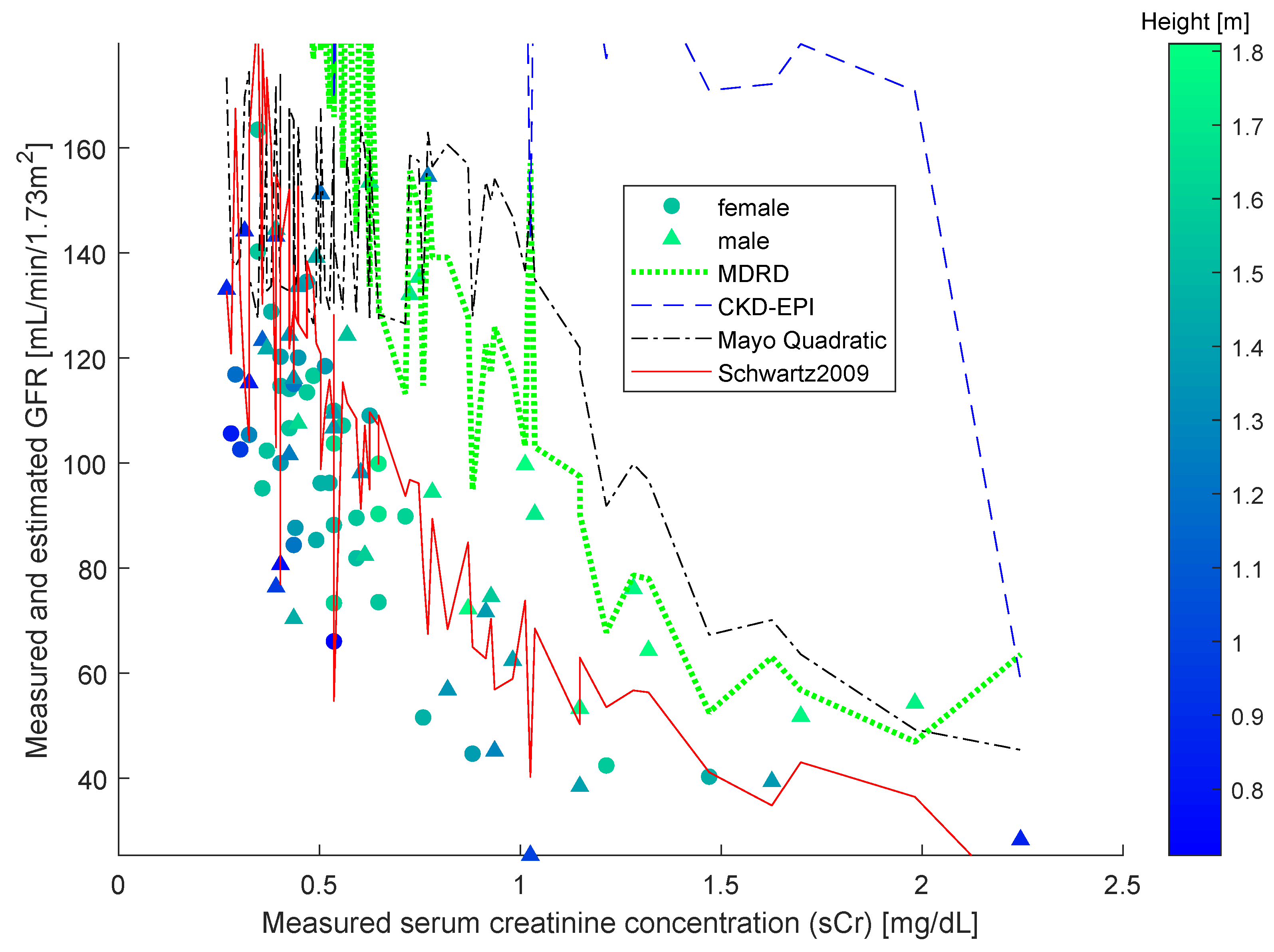
The study [38] compared four different formulas, namely, the original Schwartz formula, the updated Schwartz formula, the Filler formula and the CKiD formula. The study found the most effective estimation formula to be the updated Schwartz one. Over said data, we also computed estimations using the other three widely employed formulas, namely MDRD, CKD-EPI and Mayo Quadratic, and compared them with the results of the updated Schwartz estimation formula. From the Figure 2, it is clearly confirmed that the updated Schwartz formula outperforms all of the other functions.

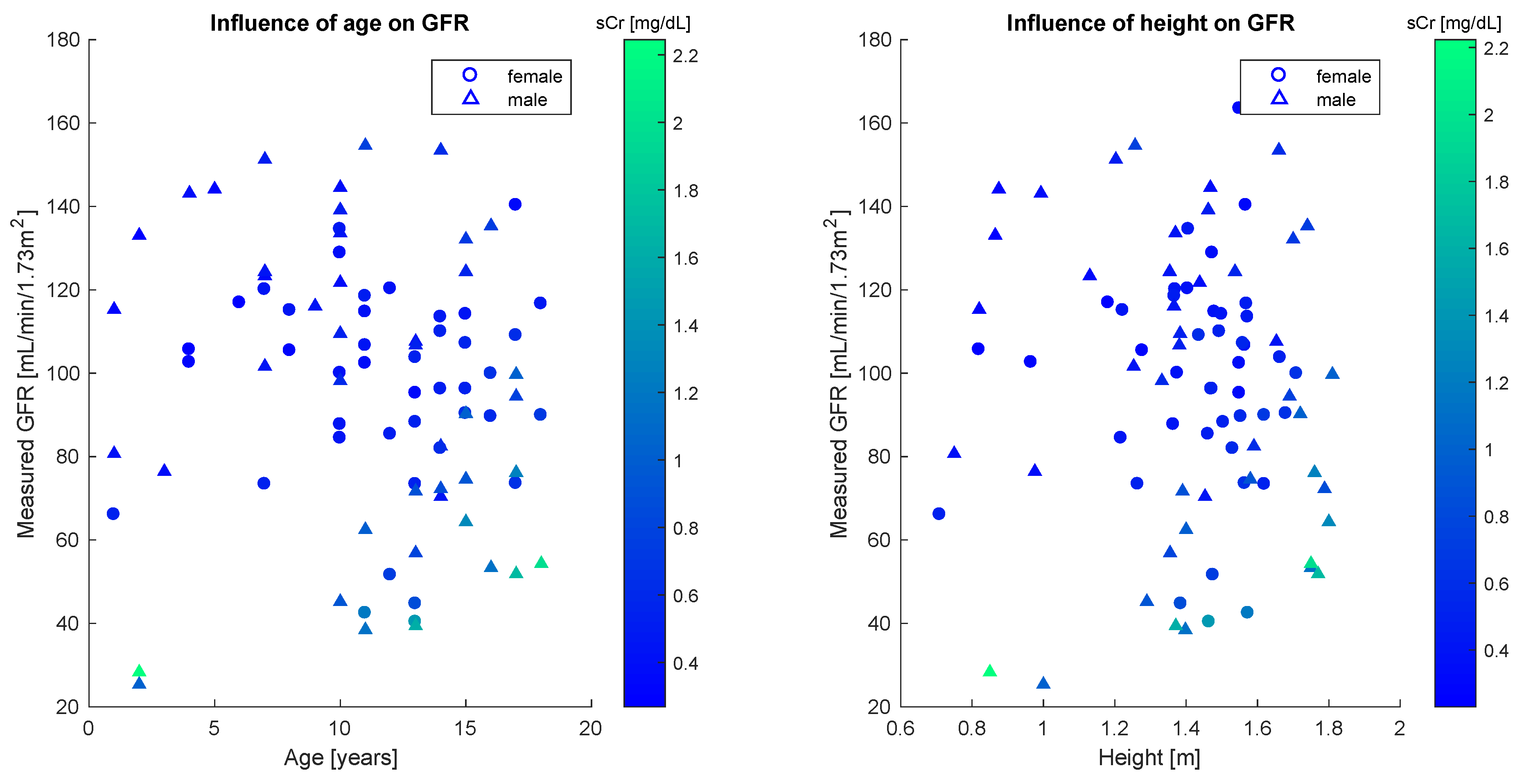
In order to apply the statistical bivariate numerical modeling algorithm developed in the Section 2, we first assessed the existence of a single dominant independent variable. This was clearly found to be the serum creatinine concentration. Other variables used to estimate the glomerular filtration rate are age and height, whose effect however is marginal, as the scatter plots in Figure 3 reveal no strong statistical features.

Quantitatively, this analysis is confirmed by the sample correlation coefficient [40].

Table 2. Sample correlation coefficients between glomerular filtration rate and age, height and creatinine concentration levels from pedriatic patients’ data. Serum creatinine concentration refers to the IMDS-traceable values.

Gender	${\mathit{\rho }}_{\mathit{GFR},\mathit{sCr}}$	${\mathit{\rho }}_{\mathit{GFR},\mathit{age}}$	${\mathit{\rho }}_{\mathit{GFR},\mathit{height}}$
Males	$-0.7051$	$-0.1375$	$-0.0910$
Females	$-0.7249$	$+0.0801$	$+0.0548$
Both	$-0.6744$	$-0.0565$	$-0.0425$

shows correlation coefficients between the GFR and each of age, height and sCr for the whole population and the gender-defined subsets. The results illustrated in the table confirm the weak statistical correlation between glomerular filtration rate and age, as well as between glomerular filtration rate and height, especially for female patients.

From the Figure 2, it is readily appreciated that the sCr–GFR relationship presents a monotonically decreasing trend, which enables us to apply the SBR numerical modeling algorithm presented in the Section 2. According to the observations drawn about the performances of the closed-form models, we did not compare the SBR numerical modeling algorithm with the MDRD, the CKD-EPI and the Mayo Quadratic formulas.

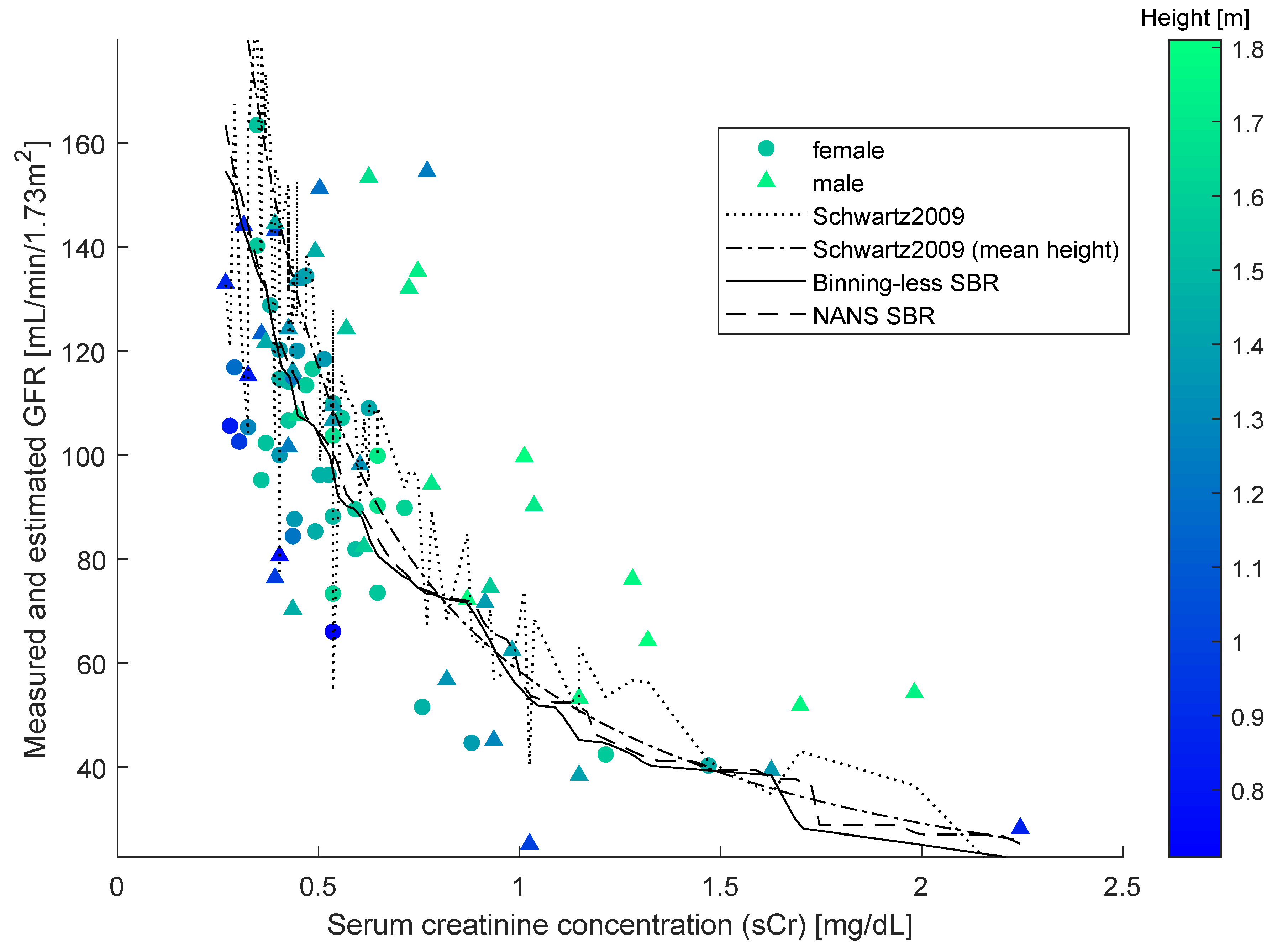
As SBR generates a bivariate numerical model, for the sake of the comparison, a simplified version of the updated Schwartz formula was introduced to be independent of height. This was done by replacing the variable height with a constant equal to the mean height of all individuals in the dataset. This model is illustrated in the Figure 4, along with the datapoints, the numerical model obtained by SBR using the numerical-algebraic neural system NANS method explained in [21], the original updated Schwartz formula and the numerical model obtained using the binning-less method described in Section 2. Notice that the GFR estimations pertaining to the updated Schwartz formula were not calculated as they were provided within the dataset.

The input-output nature of bivariate numerical modeling grants the use of functional notation (i.e., given a value for the independent variable x, the prediction made for the value of the dependent variable y can be expressed as $y=f\left(x\right)$). The notation is commonly used in reference to closed-form models and will be adopted in this paper to also indicate predictions made using the Algorithm 3 and by interpolating the curve obtained using the NANS method.

The two closed-form models and the two numerical modeling algorithms displayed in the Figure 4 were compared on prediction performance using four indexes: mean squared error (MSE), mean absolute error (MAE), variance-accounted-for (VAF) and coefficient of correlation ($\rho$), as defined in the Section 2.2. In the present context, each $x_i$ represents an instance of serum creatinine concentration sCr, each $y_i$ represents an instance of glomerular filtration rate GFR, and $n=87$.

Comparisons were also made to evaluate the generalization ability of the closed-form model (simplified Schwartz) as well as of the considered numerical numerical modeling algorithms (Binning-less SBR and NANS SBR). This was achieved by measuring the “roughness” of the the numerical models [41] through the index G defined by

$$G=\sum _{i=3}^N\frac{{(f_i-2f_{i-1}+f_{i-2})}^2}{N-2},$$

(13)

on the basis of the second-order differences of a sequence $f_i$. By definition, the index $G$ increases with sharp changes in slope. The reference value for a well-performing algorithm is $G\ge 0$ as close as possible to zero. To be useful, the $f_i$ values have to be sorted in some significant manner: in the present context, for each model $f\left(x\right)$ to be evaluated, $f_i$ assumes the predictions at $N=100$ equally spaced, increasing, values of serum creatinine concentration, namely:

$$f_i=f\left(x_{\min }+(i-1)\frac{x_{\max }-x_{\min }}{N-1}\right),\mathrm{for}i=1,\dots ,N,$$

(14)

where $x_{\min }$ and $x_{\max }$ are respectively the smallest and largest measured creatinine concentration levels. The same index cannot be applied to multivariate functions, therefore the updated Schwartz equation was not tested with this criterion. An index similar to $G$ was discussed in [42] to prevent overfitting of a neural-network model. The value of G is expected to be large for irregular curves and indeed it is close to zero for the simplified Schwartz model (independent of height), which is essentially a hyperbola, graph of a smooth function.

The results of comparison are summarized in the

Table 3. Modeling pedriatic patients’ GFR data: Generalization/roughness index ($G$), mean squared error ($\mathit{MSE}$), mean absolute error ($\mathit{MAE}$) and coefficient of correlation ($\rho$) for the four considered estimation models (updated Schwartz formula, simplified Schwartz formula independent of height, numerical-algebraic neural-system based statistical bivariate numerical modeling algorithm, and proposed statistical bivariate numerical modeling algorithm). Highlighted values denote best figures.

Models and Formulas	G	$\mathit{MSE}$	$\mathit{MAE}$	$\mathit{\rho }$	$\mathit{VAF}$ (%)	$\mathit{Runtime}$ (s)
Updated Schwartz formula	—	863.92	22.919	0.69116	23	—
Simplified Schwartz formula	0.0948	1341.80	27.519	0.63981	—	0.00116
NANS SBR model	3.2986	696.62	20.090	0.65575	30	0.00140
Binning-less SBR model	2.5806	674.90	19.952	0.66647	33	0.00085

. Notice that, in this experiment, the number N of model-points exceeds the number n of data-points. Among the four methods considered, the binning-less statistical bivariate numerical modeling algorithm exhibits the lowest $\mathit{MSE}$ and $\mathit{MAE}$ values and highest $\mathit{VAF}$ value, that shows how SBR is very effective at fitting data, as well as the lowest computation time (the $\mathit{VAF}$ value pertaining to the simplified Schwartz formula is negative and hence non-meaningful; the values pertaining to the updated Schwartz formula were provided in the dataset, hence no computation time is available for this method). Taking the G-value of the numerical model provided by the simplified Schwartz formula as a baseline, the binning-less algorithm exhibits a closer value to such baseline than the NANS SBR: this result shows that the novel SBR algorithm returns a smoother numerical model compared to the NANS SBR one.

3.3. Experimental Results on Statistical Numerical Modeling of Adult Patients Data

In this section, we illustrate and discuss experimental results about statistical numerical modeling of sCr–GFR dependency in adult patients data. The accessed data-set is a large database drawn from [43] that contains 10,610 records of mixed children, adolescents an adults. The study summarized in [43] used a dataset of subjects 3 to 90 years old, referred between July 2003 and July 2014 to a single university hospital to undergo GFR measurement for suspected or established renal dysfunction, renal risk, or before kidney donation. The exclusion criteria were being treated with dialysis at the time of the study or taking cimetidine, trimethoprim or intravenous injections of albumin or diuretics before GFR measurement. From this dataset, we excluded all those records corresponding to patients aged 18 and below, so as to isolate 9530 adults. Given the large number of data-pairs available, the numerical models were build on a training set of $90\%$ of the records and tested on a test set made of the $10\%$ remaining records, randomly selected. The number of model-points was again selected to be $N=100$ which, in this case, is far less than the number of available data-points.

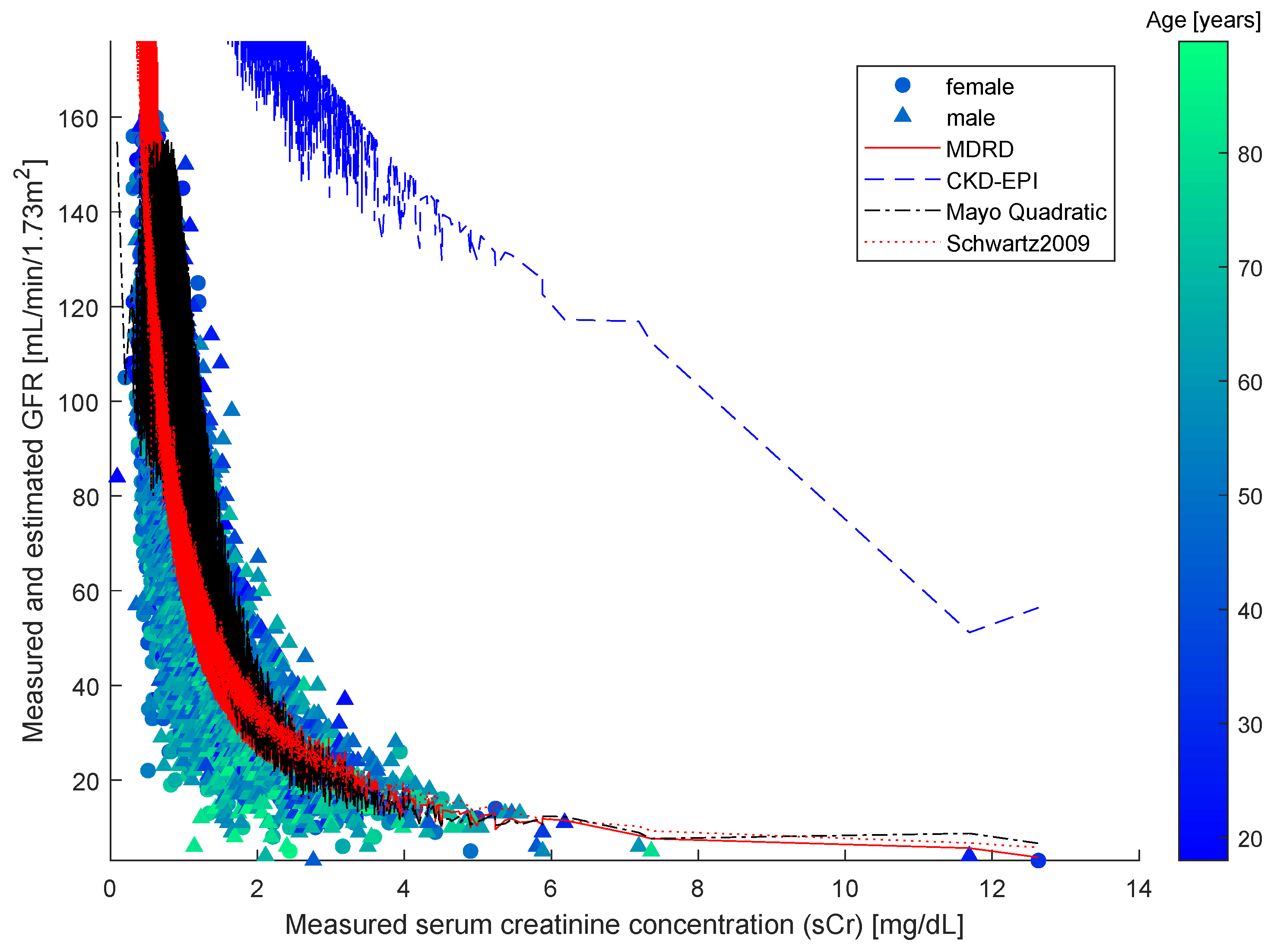
Over said data, we computed estimations using MDRD, CKD-EPI, Mayo Quadratic and updated Schwartz estimation formula. The results shown in the Figure 5 confirm the widely taken assumption that the MDRD outperforms all other models when it comes to process adult patients data.

As SBR generates a bivariate numerical model, for the sake of the comparison, a simplified version of the MDRD formula was introduced to be independent of age and gender. This was done by averaging out the age and the term in the MDRD equation that depends on the gender over the population in the dataset. The resulting models are illustrated in the Figure 6, along with testing-set datapoints.

The closed-form model and the two numerical modeling algorithms displayed in the Figure 6 were compared on prediction performance using again four indexes: mean squared error (MSE), mean absolute error (MAE), variance-accounted-for (VAF), coefficient of correlation ($\rho$) and runtime (seconds). In the present context, each $x_i$ represents an instance of serum creatinine concentration sCr, each $y_i$ represents an instance of glomerular filtration rate GFR, and $n=953$ (that is the size of the testing set).

The results of comparison are summarized in the

Table 4. Modeling adult patients’ GFR data: Generalization/roughness index ($G$), mean squared error ($\mathit{MSE}$), mean absolute error ($\mathit{MAE}$) and coefficient of correlation ($\rho$) for the four considered estimation models (simplified MDRD formula independent of age and gender, numerical-algebraic neural-system based statistical bivariate numerical modeling algorithm, and proposed statistical bivariate numerical modeling algorithm). Highlighted values denote best figures.

Models and Formulas	G	$\mathit{MSE}$	$\mathit{MAE}$	$\mathit{\rho }$	$\mathit{VAF}$ (%)	$\mathit{Runtime}$ (s)
Simplified MDRD	120.38	440.61	14.510	0.8149	52	0.00800
NANS SBR model	2.82	345.14	14.165	0.7884	58	0.06953
Binning-less SBR model	3.17	358.38	14.438	0.7854	57	0.00485

. Among the three methods considered, the statistical bivariate numerical modeling algorithms (NANS SBR and Binning-less SBR) exhibits the lowest $\mathit{MSE}$ and $\mathit{MAE}$ values and the highest $\mathit{VAF}$ values, which shows how SBR methods are effective at fitting data. The extremely large value of the roughness G exhibited by the Simplified MDRD method is due to the fact that, for low values creatinine (say, for $sCr<1$), the model is unreliable, as can be directly seen from the Figure 6. The last column of the Table 4 evidences how the Binning-less SBR algorithm is not only way more efficient than the older version (NANS SBR), but even of the Simplified MDRD formula. Since the performances exhibited by the old version of the modeling algorithm (NANS SBR) and the newest version proposed in this paper (Binning-less SBR) are very close to one another, but the computational complexity of the latter is lesser than the former, we drew the conclusion that the novel, simplified version is preferable to the older.

Example 2.

In order to highlight the practical usage of the developed SBR modeling procedure, we discuss here an example of how a numerical model may be taken advantage of to infer the glomerular filtration rate from a serum creatinine assay. The

Table 5. Portion of a numerical model obtained on the adult patients sCR/GFR dataset. Two rows enclosed in a red box represent two data-pairs used in the interpolation of the reading ${\mathrm{sCR}}^{\star }=2.02$ in the Example 2.

sCr (mg/mL)	GFR (mL/min/1.73 m2)
⋮	⋮
1.2300	53.9677
1.3567	47.5155
1.4833	43.0885
1.6100	38.7733
1.7367	34.5119
1.8633	31.1092
1.9900	28.6909
2.1167	26.2985
2.2433	24.5742
2.3700	22.9250
⋮	⋮

shows a portion of the SBR model inferred on the adult patients dataset. The whole model includes 100 sCR–GFR pairs and the table shows 10 pairs for sCr ranging in $[1.23,2.37]$. As a numerical example, one may assume a reading of ${\mathrm{sCR}}^{\star }=2.02$. The nearest values in the table are sCr $=1.99$ and sCr $=2.11$, to which correspond GFR $=28.6909$ and GFR $=26.2985$, respectively. By a linear interpolation, one gets the linear equation

$$\frac{{\mathrm{GFR}}^{\star }-26.2985}{2.02-2.11}=\frac{28.6909-26.2985}{1.99-2.11},$$

that leads to the estimation ${\mathrm{GFR}}^{\star }=28.0928$. The actual value in the dataset is ${\mathrm{GFR}}^{\star }=29.0000$, hence the prediction by the model is off of about $3\%$. Notice that the newly acquired value of serum creatinine may be merged to the sCr dataset in order to make the CDF estimation—and hence the model predictions—more accurate the next time.

4. Conclusions

The aim of the present paper is to discuss the statistical bivariate numerical modeling method and to provide an improved algorithm which does not rely on binning for the steps that require estimation of the cumulative distribution functions.

The proposed algorithm was compared to the original statistical bivariate numerical modeling algorithm based on numerical-algebraic neural systems in the application to benchmark as well as to real-world datasets. The application that motivated the present research is the estimation of an index of kidney function, the glomerular filtration rate, on the basis of numerical modeling by the creatinine concentration level in blood plasma. The results of comparisons proved an improvement in the new method in terms of computational efficiency.

The algorithm proposed in the present paper will be subjected to future investigations aiming at improving its applicability and in reducing its computational complexity. During the review process, it was suggested that the Algorithm 1 could be asymptotically improved in complexity: The current version of the algorithm performs a binary search (after sorting) by a $O\left(n\right)$ complexity, while binary search by divide & conquer can be performed in $O(logn)$. Moreover, it was suggested that sorting could allegedly be simplified, which would reduce the overall complexity to $O\left(n\right)$ (as in the main text, n denotes the cardinality of a dataset). Moreover, the current version of the numerical modeling algorithm is inherently unable to cope with non-monotonic relationships between data: we are currently working towards an extension of the underlying theory to non-isotonic binning-less statistical numerical modeling.

References

- Gao, D. Texture model regression for effective feature discrimination: Application to seismic facies visualization and interpretation. Geophysics 2004, 69, 958–967. [Google Scholar] [CrossRef]
- Carrara, P.; Altamura, E.; D’Angelo, F.; Mavelli, F.; Stano, P. Measurement and numerical modeling of cell-free protein synthesis: Combinatorial block-variants of the PURE system. Data 2018, 3, 41. [Google Scholar] [CrossRef]
- McArthur, J.M.; Howarth, R.J.; Bailey, T.R. Strontium isotope stratigraphy: LOWESS version 3: Best fit to the marine Sr-isotope curve for 0-509 Ma and accompanying look-up table for deriving numerical age. J. Geol. 2001, 109, 155–170. [Google Scholar] [CrossRef]
- Xu, L.; Li, C.; Xie, X.; Zhang, G. Long-short-term memory network based hybrid model for short-term electrical load forecasting. Information 2018, 9, 165. [Google Scholar] [CrossRef]
- Gill, J.; Malyuk, R.; Djurdjev, O.; Levin, A. Use of GFR equations to adjust drug doses in an elderly multi-ethnic group—A cautionary tale. Nephrol. Dial. Transplant. 2007, 22, 2894–2899. [Google Scholar] [CrossRef] [PubMed]
- Matsushita, K.; van der Velde, M.; Astor, B.C.; Woodward, M.; Levey, A.S.; de Jong, P.E.; Coresh, J.; Gansevoort, R.T. Association of estimated glomerular filtration rate and albuminuria with all-cause and cardiovascular mortality in general population cohorts: A collaborative meta-analysis. Lancet 2010, 375, 2073–2081. [Google Scholar] [PubMed]
- Endre, Z.H.; Pickering, J.W.; Walker, R.J. Clearance and beyond: the complementary roles of GFR measurement and injury biomarkers in acute kidney injury (AKI). Am. J. Physiol. Ren. Physiol. 2011, 301, 697–707. [Google Scholar] [CrossRef] [PubMed]
- Soveri, I.; Berg, U.B.; Björk, J.; Elinder, C.G.; Grubb, A.; Mejare, I.; Sterner, G.; Bäck, S.E. Measuring GFR: A systematic review. Am. J. Kidney Dis. 2014, 64, 411–424. [Google Scholar] [CrossRef] [PubMed]
- Verhees, B.; van Kuijk, K.; Simonse, L. Care model design for e-Health: integration of point-of-care testing at Dutch general practices. Int. J. Environ. Res. Public Health 2018, 15, 4. [Google Scholar] [CrossRef] [PubMed]
- Kopp, R.E.; Orford, R.J. Linear regression applied to system identification for adaptive control systems. Am. Inst. Aeronaut. Astronaut. J. 1963, 1, 2300–2306. [Google Scholar] [CrossRef]
- Masry, E. Multivariate local polynomial regression for time series: uniform strong consistency and rates. J. Time Ser. Anal. 1996, 17, 571–599. [Google Scholar] [CrossRef]
- Harrell, F.E. Regression Modeling Strategies: With Applications to Linear Models, Logistic and Ordinal Regression, and Survival Analysis; Springer Series in Statistics; Springer: New York, NY, USA, 2015. [Google Scholar]
- Shi, L.; Li, Y.; Feng, H. Performance analysis of honeypot with Petri nets. Information 2018, 9, 245. [Google Scholar] [CrossRef]
- Li, G.; Ma, X.; Yang, H. A hybrid model for monthly precipitation time series forecasting based on variational mode decomposition with extreme learning machine. Information 2018, 9, 177. [Google Scholar] [CrossRef]
- Yue, B.; Fu, J.; Liang, J. Residual recurrent neural networks for learning sequential representations. Information 2018, 9, 56. [Google Scholar] [CrossRef]
- Liu, X.; Pei, X.; Li, N.; Zhang, Y.; Zhang, X.; Chen, J.; Lv, L.; Ma, H.; Wu, X.; Zhao, W.; et al. Improved glomerular filtration rate estimation by an artificial neural network. PLoS ONE 2013, 8, e58242. [Google Scholar] [CrossRef] [PubMed]
- Liu, X.; Li, N.S.; Lv, L.S.; Huang, J.H.; Tang, H.; Chen, J.X.; Ma, H.J.; Wu, X.M.; Lou, T.Q. A comparison of the performances of an artificial neural network and a regression model for GFR estimation. Am. J. Kidney Dis. 2013, 62, 1109–1115. [Google Scholar] [CrossRef] [PubMed]
- Janssen, I.; Katzmarzyk, P.T.; Ross, R. Waist circumference and not body mass index explains obesity-related health risk. Am. Soc. Clin. Nutr. 2004, 79, 379–384. [Google Scholar] [CrossRef] [PubMed]
- Best, M.J.; Chakravarti, N. Active set algorithms for isotonic regression; a unifying framework. Math. Program. 1990, 47, 425–439. [Google Scholar] [CrossRef]
- Mair, P.; Hornik, K.; de Leeuw, J. Isotone optimization in R: pool-adjacent-violators algorithm (PAVA) and active set methods. J. Stat. Softw. 2009, 32, 1–24. [Google Scholar]
- Fiori, S. Fast statistical regression in presence of a dominant independent variable. Neural Comput. Appl. 2013, 22, 1367–1378. [Google Scholar] [CrossRef]
- Fiori, S.; Gong, T.; Lee, H.K. Bivariate nonisotonic statistical regression by a lookup table neural system. Cogn. Comput. 2015, 7, 715–730. [Google Scholar] [CrossRef]
- Abiodun, O.I.; Jantan, A.; Omolara, A.E.; Dada, K.V.; Mohamed, N.A.; Arshad, H. State-of-the-art in artificial neural network applications: A survey. Heliyon 2018, 4, e00938. [Google Scholar] [CrossRef] [PubMed]
- Yang, W.; Wang, J.; Wang, R. Research and application of a novel hybrid model based on data selection and artificial intelligence algorithm for short term load forecasting. Entropy 2017, 19, 52. [Google Scholar] [CrossRef]
- Criminisi, A.; Shotton, J. Regression forests. In Decision Forests for Computer Vision and Medical Image Analysis; Advances in Computer Vision and Pattern, Recognition; Criminisi, A., Shotton, J., Eds.; Springer: London, UK, 2013. [Google Scholar] [CrossRef]
- Laskin, B.L.; Nehus, E.; Goebel, J.; Khoury, J.C.; Davies, S.M.; Jodele, S. Cystatin C-estimated glomerular filtration rate in pediatric autologous hematopoietic stem cell transplantation. Biol. Blood Marrow Transplant. 2012, 18, 1745–1752. [Google Scholar] [CrossRef] [PubMed]
- Slot, C. Plasma creatinine determination a new and specific Jaffe reaction method. Scand. J. Clin. Lab. Investig. 1965, 17, 381–387. [Google Scholar] [CrossRef] [PubMed]
- Welch, M.J.; Cohen, A.; Hertz, H.S.; Ng, K.J.; Schaffer, R.; van der Lijn, P.; White, E. Determination of serum creatinine by isotope dilution mass spectrometry as a candidate definitive method. Anal. Chem. 1986, 58, 1681–1685. [Google Scholar] [CrossRef] [PubMed]
- Levey, A.S.; Bosch, J.P.; Lewis, J.B.; Greene, T.; Rogers, N.; Roth, D. A more accurate method to estimate glomerular filtration rate from serum creatinine: A new prediction equation. Modification of Diet in Renal Disease Study Group. Ann. Intern. Med. 1999, 130, 461–470. [Google Scholar] [CrossRef] [PubMed]
- Rule, A.D.; Larson, T.S.; Bergstralh, E.J.; Slezak, J.M.; Jacobsen, S.J.; Cosio, F.G. Using serum creatinine to estimate glomerular filtration rate: accuracy in good health and in chronic kidney disease. Ann. Intern. Med. 2004, 141, 929–937. [Google Scholar] [CrossRef] [PubMed]
- Levey, A.S.; Stevens, L.A.; Schmid, C.H.; Zhang, Y.L.; Castro, A.F.; Feldman, H.I.; Kusek, J.W.; Eggers, P.; van Lente, F.; Greene, T.; et al. A new equation to estimate glomerular filtration rate. Ann. Intern. Med. 2009, 150, 604–612. [Google Scholar] [CrossRef] [PubMed]
- Rigalleau, V.; Lasseur, C.; Raffaitin, C.; Perlemoine, C.; Barthe, N.; Chauveau, P.; Combe, C.; Gin, H. The Mayo clinic quadratic equation improves the prediction of glomerular filtration rate in diabetic subjects. Nephrol. Dial. Transplant. 2007, 22, 813–818. [Google Scholar] [CrossRef] [PubMed]
- Counahan, R.; Chantler, C.; Ghazali, S.; Kirkwood, B.; Rose, F.; Barratt, T.M. Estimation of glomerular filtration rate from plasma creatinine concentration in children. Arch. Dis. Child. 1976, 51, 875–878. [Google Scholar] [CrossRef] [PubMed]
- Grubb, O.S.A.; Thysell, H. The blood serum concentration of cystatin C (gamma-trace) as a measure of the glomerular filtration rate. Scand. J. Clin. Lab. Investig. 1985, 45, 97–101. [Google Scholar]
- Schwartz, G.J.; Mu noz, A.; Schneider, M.F.; Mak, R.H.; Kaskel, F.; Warady, B.A.; Furth, S.L. New equations to estimate GFR in Children with CKD. J. Am. Soc. Nephrol. 2009, 20, 629–637. [Google Scholar] [CrossRef] [PubMed]
- Grubb, A.; Blirup-Jensen, S.; Lindstrom, V.; Schmidt, C.; Althau, H.; Zegers, I. First certified reference material for cystatin C in human serum ERM-DA471/IFCC. Clin. Chem. Lab. Med. 2010, 48, 1619–1621. [Google Scholar] [CrossRef] [PubMed]
- Schwartz, G.J.; Schneider, M.F.; Maier, P.S.; Moxey-Mims, M.; Dharnidharka, V.R.; Warady, B.A.; Furth, S.L.; Muñoz, A. Improved equations estimating GFR in children with chronic kidney disease using an immunonephelometric determination of cystatin C. Kidney Int. 2012, 82, 445–453. [Google Scholar] [CrossRef] [PubMed]
- Zheng, K.; Gong, M.; Qin, Y.; Song, H.; Shi, X.; Wu, Y.; Li, F.; Li, X. Validation of glomerular filtration rate-estimating equations in Chinese children. PLoS ONE 2017, 12, e0180565. [Google Scholar] [CrossRef] [PubMed]
- Serdar, M.A.; Kurt, I.; Ozcelik, F.; Urhan, M.; Ilgan, S.; Yenicesu, M.; Kutluay, T. A practical approach to glomerular filtration rate measurements: Creatinine clearance estimation using cimetidine. Ann. Clin. Lab. Sci. 2001, 31, 265–273. [Google Scholar] [PubMed]
- Mukaka, M.M. A guide to appropriate use of correlation coefficient in medical research. Malawi Med. J. 2012, 24, 69–71. [Google Scholar] [PubMed]
- He, X.; Ng, P.; Portnoy, S. Bivariate quantile smoothing splines. J. R. Stat. Soc. Ser. B Stat. Methodol. 1998, 60, 537–550. [Google Scholar] [CrossRef]
- Bishop, C.M. Training with noise is equivalent to Tikhonov regularization. Neural Comput. 1995, 7, 108–116. [Google Scholar] [CrossRef]
- Da Silva Selistre, L. Replication Data for: Comparison of Schwartz and CDK-EPI Equations for Estimating GFR in Children, Adolescents, and Adults: A Retrospective Cross-Sectional Study, Harvard Dataverse, Version 2; Deposit Date: 15 December 2015; Available online: https://dataverse.harvard.edu/dataset.xhtml?persistentId=doi:10.7910/DVN/SKSPSY (accessed on 6 March 2019).
Figure 1.
Comparison on modeling a polynomial dependency made using numerical-algebraic neural-system based statistical bivariate numerical modeling algorithm (NANS SBR), the proposed binning-less statistical bivariate numerical modeling algorithm, an artificial neural network, a support vector regression algorithm and random-trees algorithm.
Figure 2.
Comparison of predictions made using different equations (MDRD, CKD-EPI, Mayo Quadratic and updated Schwartz) on a pedriatic patients’ dataset. The serum creatinine concentration refers to the IMDS-traceable values.
Figure 3.
Scatter plots of the glomerular filtration rate versus pediatric patients age or height suggest weak correlation. Serum creatinine concentration refers to the IMDS-traceable values.
Figure 4.
Pedriatic patients’ GFR data set with overlaid numerical model and estimation curves. Comparison of the updated Schwartz equation, the simplified Schwartz equation, the Numerical-Algebraic Neural System (NANS) method introduced in [21] and the proposed method. Serum creatinine concentration refers to the IDMS-traceable values.
Figure 5.
Comparison of predictions made using different equations (MDRD, CKD-EPI, Mayo Quadratic and updated Schwartz) on an adults dataset.
Figure 6.
Adults data set with overlaid numerical model and estimation curve. Comparison of the Simplified MDRD, the SBR NANS and the proposed Binning-less SBR (on a testing set only).