Optimal Control of Virus Spread under Different Conditions of Resources Limitations ^†

Abstract

The paper addresses the problem of human virus spread reduction when the resources for the control actions are somehow limited. This kind of problem can be successfully solved in the framework of the optimal control theory, where the best solution, which minimizes a cost function while satisfying input constraints, can be provided. The problem is formulated in this contest for the case of the HIV/AIDS virus, making use of a model that considers two classes of susceptible subjects, the wise people and the people with incautious behaviours, and three classes of infected, the ones still not aware of their status, the pre-AIDS patients and the AIDS ones; the control actions are represented by an information campaign, to reduce the category of subjects with unwise behaviour, a test campaign, to reduce the number of subjects not aware of having the virus, and the medication on patients with a positive diagnosis. The cost function considered aims at reducing patients with positive diagnosis using as less resources as possible. Four different types of resources bounds are considered, divided into two classes: limitations on the instantaneous control and fixed total budgets. The optimal solutions are numerically computed, and the results of simulations performed are illustrated and compared to put in evidence the different behaviours of the control actions.

1. Introduction

In this paper, an optimal control approach to to limit the spread of the Human Immunodeficiency Virus (HIV), and then of the Acquired Immune Deficiency Syndrome (AIDS), is proposed, under the constraints given by resources limitation.

The problem of optimal resources management, especially when they are constrained or limited, is a challenging task in several fields, Refs. [1,2,3,4,5,6,7]. For example, in [1], the limited resources are the data received over a network to be used for system identifications. Also in [2], the problem of resource allocation is referred to constrained communication over networks, and the resources are represented by the channels over which the information are exchanged. A totally different case, with the same problem of optimal resources allocation, is referred in [3]: there, the sectors of material production and human capital are addressed. Natural resources are another large field of applications: in this case, one refers to energetic sources, fuels, especially fossil, or water, as in [4]. Also in medical and healthcare contests, the problem of optimal allocation of the limited resources is crucial for maximising the population wellness [5]. In these cases, the resources can be heterogeneous entities: physical devices and equipments, spaces and locations, such as operating rooms or beds in hospitals, medical and paramedical staff, and so on. In the framework of non linear analysis, in [6] the classical Susceptible Infected Removed (SIR) epidemic model is studied in the complex case of resource limitations, including non linear impulsive function. For the case here addressed, the HIV/AIDS spread, the resources can be intended at a higher level as the money to invest to actuate the controls; but they can also be the units of medicaments or the single blood test kit. In [7] the problem of the HIV transmission is considered along with the tuberculosis diffusion, studying the limitations of the resources and their optimal allocations.

HIV is responsible of the AIDS, that can be reached after 10–15 years from the infection [8,9,10]. The HIV is mainly transmitted through body fluids exchange between individuals; the virus infects cells, weakening them so that the possibility of a generic infection increases. The modalities of its diffusion are well-know; its spread could be limited adopting wise behaviours between the susceptible individuals. A dangerous aspect of this pathology is the delay for the infected subjects to become aware of their status; during this long time interval, they can be highly contagious. No effective vaccine exists up to now, only medication after the positive response to HIV- test. An information campaign could induce people to have cautious behaviours and to periodically test their negativeness to the HIV/AIDS. Moreover, medication is included in the control actions since new drug therapies help the patients in remaining in the HIV situations without reaching the AIDS status. These three levels of intervention are suggested by the World Health Organization (WHO).

Mathematical modelling of the HIV/AIDS diffusion has been faced in [9,10,11,12,13,14,15,16,17], by considering, as in this paper, the dynamics between subjects, thus introducing:

-

the class of susceptible subjects (S) that are the healthy individuals that may contract the virus;

-

the class of the infected individuals (I) not aware of their condition;

-

the class of the pre-AIDS patients (P);

-

the class of the AIDS patients (A).

The importance of prevention has been stated in [12,13], where the attention is devoted to risky subjects, drug users and sex workers, showing with simulation the effects of prevention.

The natural framework to study epidemic problems is the optimal control, aiming at determining the best action with respect to conflicting requirements, such as using as less resources as possible while maximising the effects, that is minimizing the number of infected patients, Refs. [15,17,18,19,20,21].

In this paper, the approach considering the dynamics of the interactions between subjects [8,11,12] is adopted. The susceptible individuals S are divided into two categories, considering people adopting wise behaviours and the ones that do not consider adequately the dangerousness of this disease. Therefore, five categories are present: two classes of healthy subjects and three classes of subjects with HIV/AIDS. It is worth to be noted that only the pre-AIDS subjects and the AIDS patients are actually aware of their status. The external actions introduced are an effective information campaign, a test campaign and the virus therapy. The control laws are computed to minimize a cost index which depends on the state and the controls. Its aim is to reduce the number of infected subjects with positive diagnosis of HIV/AIDS under different constraints on the control action.

In [17], the authors considered one hypothesis on the resources bounds, the classical case of instantaneous limitation on each input, usually used when the control has some upper and/or lower bound.

Here, three other cases are also studied: the case of instantaneous limitation on the sum of the controls, when a common resource, which has to be divided for the different controls, is characterized by bounds, the case of a total budget for each control, to be distributed optimally along the time of the control action, and a final case of a total budget to be distributed among the inputs and modulated over the time actions.

The paper is organized as follows. In Section 2 the mathematical model is shortly recalled and the optimal control problem is formulated for the four cases of constraints investigated. Section 3 is devoted to report and discuss the results of numerical simulations carried on to check the designed controls actions and to compare their behaviour under the different constraints. In Section 4 a conclusive discussion of the results obtained is proposed.

2. The Mathematical Model, the Optimal Control Problem Formulation and Its Solution

In this section, the mathematical model of the HIV/AIDS spread here adopted is recalled and its main characteristics are explained in Section 2.1. Then, the optimal control problem is formulated for four different types of constraints on the controls, i.e., on the resources available, and solved.

2.1. The HIV/AIDS Model

The model of the HIV/AIDS diffusion presented and used in [12,13,17] is here briefly recalled. This disease is particularly dangerous since there is a period, also ten years long, in which its symptoms are not evident and therefore a subject could, unconsciously, infect other people. Nevertheless, it could be transmitted only by specific risky contacts; despite the fact that all the subjects could contract the virus, with wise behaviours the infection could be stopped. These two characteristics have been considered in the WHO suggestions of intervention and have guided the choices of the proposed modelling.

In particular, the healthy people are divided into two categories: the unwary individuals, denoted by $S_1$, and the wise ones that adopt safe behaviours, named $S_2$. The infected subjects may be distinguished into three kinds of patients: the ones that still do not know to be infected, I, those with a positive HIV diagnosis, P, and the ones with AIDS, A. The control actions introduced are the prevention with information campaign inducing subjects to wise behaviours and to improve a test campaign (primary and secondary preventions, respectively); moreover, the medication is applied on the patients with positive HIV/AIDS diagnosis (third action). The costs of primary and secondary preventions represent an immediate economic effort, whereas the effects could be noted only in the future: a schedule of the control action is advisable.

Let $S_1\left(t\right)$, $S_2\left(t\right)$, $I\left(t\right)$, $P\left(t\right)$ and $A\left(t\right)$ denote the number of individuals in each of the previous categories. It is useful to introduce also the quantity $N_c\left(t\right)=S_1\left(t\right)+S_2\left(t\right)+I\left(t\right)$, representing the part of the population for which no diagnosis has been produced; it is the sum of the healthy people and the unaware ones.

In Figure 1, the block diagram representing the interactions described above is depicted.

The control actions introduced are: $u_1\left(t\right)$, corresponding to the effort placed in the information campaign for the $S_1\left(t\right)$ reduction; $u_2\left(t\right)$, that is related to a test campaign to reduce the unaware infected individuals and, consequently, to reduce the interaction responsible of the epidemic spread; $u_3\left(t\right)$, the therapy, which reduces the transition of the known infected individuals $P\left(t\right)$ to the terminal group $A\left(t\right)$.

Therefore, the final model is:

$$\begin{array}{ccc}\hfill {\dot{S}}_1\left(t\right)& =& Z-d{S}_1\left(t\right)-\beta \frac{S_1\left(t\right)I\left(t\right)}{N_c\left(t\right)}+\gamma S_2\left(t\right)-S_1\left(t\right)u_1\left(t\right)\hfill \end{array}$$

(1)

$$\begin{array}{ccc}\hfill {\dot{S}}_2\left(t\right)& =& -\left(\gamma +d\right)S_2\left(t\right)+S_1\left(t\right)u_1\left(t\right)\hfill \end{array}$$

(2)

$$\begin{array}{ccc}\hfill \dot{I}\left(t\right)& =& \beta \frac{S_1\left(t\right)I\left(t\right)}{N_c\left(t\right)}-\left(d+\delta \right)I\left(t\right)-\psi \frac{I\left(t\right)}{N_c\left(t\right)}{u}_2\left(t\right)\hfill \end{array}$$

(3)

$$\begin{array}{ccc}\hfill \dot{P}\left(t\right)& =& \epsilon \delta I\left(t\right)-\left(\alpha +d\right)P\left(t\right)+\varphi \psi \frac{I\left(t\right)}{N_c\left(t\right)}{u}_2\left(t\right)+P\left(t\right)u_3\left(t\right)\hfill \end{array}$$

(4)

$$\begin{array}{ccc}\hfill \dot{A}\left(t\right)& =& (1-\epsilon )\delta I\left(t\right)+\alpha P\left(t\right)-\left(\mu +d\right)A\left(t\right)+(1-\varphi )\psi \frac{I\left(t\right)}{N_c\left(t\right)}{u}_2\left(t\right)-P\left(t\right)u_3\left(t\right)\hfill \end{array}$$

(5)

where Z denotes the rate of increment of the population, assumed as healthy newcomers, nor aware of the disease.

For sake of simplicity, sometimes it can be useful to refer to the dynamics (1)–(5) in a compact form. Defining the state vector

$$x\left(t\right)={\left(\begin{array}{ccccc}{S}_1\left(t\right)& S_2\left(t\right)& I\left(t\right)& P\left(t\right)& A\left(t\right)\end{array}\right)}^T$$

(6)

and the control vector

$$u\left(t\right)={\left(\begin{array}{ccc}{u}_1\left(t\right)& u_2\left(t\right)& u_3\left(t\right)\end{array}\right)}^T$$

(7)

it is possible to write Equations (1)–(5) as

$$\dot{x}\left(t\right)=f\left(x\left(t\right)\right)+\left(\begin{array}{ccc}{g}_1\left(x\left(t\right)\right)& g_2\left(x\left(t\right)\right)& g_3\left(x\left(t\right)\right)\end{array}\right)u\left(t\right)$$

(8)

where

$$f\left(x\left(t\right)\right)=\left(\begin{array}{c}Z-d{S}_1\left(t\right)-\beta \frac{S_1\left(t\right)I\left(t\right)}{N_c\left(t\right)}+\gamma S_2\left(t\right)\\ -\left(\gamma +d\right)S_2\left(t\right)\\ \beta \frac{S_1\left(t\right)I\left(t\right)}{N_c\left(t\right)}-\left(d+\delta \right)I\left(t\right)\\ \epsilon \delta I\left(t\right)-\left(\alpha +d\right)P\left(t\right)\\ (1-\epsilon )\delta I\left(t\right)+\alpha P\left(t\right)-\left(\mu +d\right)A\left(t\right)\end{array}\right)$$

(9)

$$g_1\left(x\left(t\right)\right)=\left(\begin{array}{c}-S_1\left(t\right)\\ S_1\left(t\right)\\ 0\\ 0\\ 0\end{array}\right),g_2\left(x\left(t\right)\right)=\left(\begin{array}{c}0\\ 0\\ -\psi \frac{I\left(t\right)}{N_c\left(t\right)}\\ \varphi \psi \frac{I\left(t\right)}{N_c\left(t\right)}\\ (1-\varphi )\psi \frac{I\left(t\right)}{N_c\left(t\right)}\end{array}\right),g_3\left(x\left(t\right)\right)=\left(\begin{array}{c}0\\ 0\\ 0\\ P\left(t\right)\\ -P\left(t\right)\end{array}\right)$$

(10)

All the parameters appearing in (1)–(5) represent the coefficients which weight each contribution to the correspondent rate of variables change. In particular

-

$\beta$ regulates the interaction responsible of the infectious propagation;

-

$\gamma$ takes into account the fact that a wise individual in $S_2\left(t\right)$ can, accidentally, assume a incautious behaviour as the $S_1\left(t\right)$ persons;

-

$\delta$ weights the natural rate of $I\left(t\right)$ subjects becoming aware of their status;

-

$\alpha$ characterizes the natural rate of transition from $P\left(t\right)$ to $A\left(t\right)$ due to the evolution of the infectious disease;

-

$\psi$ determines the effect of the test campaign on the unaware individuals $I\left(t\right)$;

-

$\varphi$ is the fraction of individuals in $I\left(t\right)$ which become, after test, classified as $P\left(t\right)$ ($\varphi$) or $A\left(t\right)$ ((1 − $\varphi$));

-

$\epsilon$ is the fraction of individuals $I\left(t\right)$ which discover to be in the pre-AIDS condition or in the AIDS one;

-

d is responsible of the natural death rate, assumed the same for all the classes, while $\mu$ is the additional death factor for the individuals $A\left(t\right)$.

2.2. The Optimal Control

In the model (1)–(5), the number of subjects $P\left(t\right)$ with positive diagnosis of HIV and the one $A\left(t\right)$ with AIDS is an information that could be reasonably assumed known, resulting after specific tests. A cost index aiming at the minimization of the number of patients $P\left(t\right)$ and $A\left(t\right)$ is then introduced; this should imply an indirect effect also on the unknown number $I\left(t\right)$ and on the number of $S_1\left(t\right)$ subjects, by introducing effective control actions.

In the definition of the control problem, the time interval $t\in [0,t_f]$ is considered, with $t_f$ fixed; the final state is left free, while the initial state is assumed fixed and known:

$$x_0=x\left(0\right)={\left(\begin{array}{ccccc}{S}_1\left(0\right)& S_2\left(0\right)& I\left(0\right)& P\left(0\right)& A\left(0\right)\end{array}\right)}^T$$

(11)

Realistic considerations suggest the introduction of a limitation on the resources needed. In [17] such a limitation was defined by an instantaneous upper bound for each control; in the present work, different hypotheses on the resources bound are considered, according to instantaneous or global limitations. The following four cases can be considered, where the point $i.$ is the one already used in [17]:

i.

each control $u_i\ge 0$ is bounded, at each time instant, by an upper limit;

ii.

the instantaneous total control effort, given by the sum, at each time instant, of all the controls, is bounded by a total upper limit;

iii.

the total control effort of each input, measured by its integral over all the action time $[0,t_f]$, is equal to a prefixed value;

iv.

the total control effort of all the inputs over the action time interval $[0,t_f]$ is equal to a global value.

A cost index is introduced; the general form here adopted considers the time integral of terms quadratic both with respect to the state x and with respect to the control input u:

$$J\left(x,u\right)=\frac{1}{2}{\int }_0^{t_f}\left(x^{T}Qx+u^{T}Ru\right)dt,$$

(12)

with Q a positive semi-definite matrix and R a positive definite one. The entries of both Q and R are detailed hereinafter according to the designing specifications.

The goal is to determine the control u and the state evolution x that minimize the cost index (12) and satisfy the system (1)–(5) with the initial conditions (11). Four different particular problems are defined, one for each of the hypotheses $i.$–$iv.$. They are developed and solved in the next four subsections.

2.3. Problem Formulation for Case i

In this case the control is subject to the constraints

$$0\le u_i\left(t\right)\le U_i,t\in [0,t_f],U_i\in \Re ,i=1,2,3.$$

(13)

The weight matrix Q is defined as

$$Q=\mathit{diag}\{0,0,0,a_1,a_2\}$$

(14)

meaning that the minimization of the diagnosed infected individuals, the measurable ones among the infected, is the desired goal. With regards to R, a full rank diagonal matrix

$$R=\mathit{diag}\{r_1,r_2,r_3\}$$

(15)

is chosen.

To solve the minimization problem, the Hamiltonian function

$$H=\frac{1}{2}\left(x^{T}Qx+u^{T}Ru\right)+{\lambda }^T\left(f\left(x\right)+\sum _{i=1}^3{g}_i\left(x\right)u_i\right)$$

(16)

is introduced, where

$$\lambda \left(t\right)={\left(\begin{array}{ccccc}{\lambda }_1\left(t\right)& {\lambda }_2\left(t\right)& {\lambda }_3\left(t\right)& {\lambda }_4\left(t\right)& {\lambda }_5\left(t\right)\end{array}\right)}^T\in {\Re }^5$$

(17)

is the costate function. The explicit expression of (16) is

$$\begin{array}{ccc}\hfill H& =& \frac{1}{2}\left(a_1{P}^2\left(t\right)+a_2{A}^2\left(t\right)+r_1{u}_1^2\left(t\right)+r_2{u}_2^2\left(t\right)+r_3{u}_3^2\left(t\right)\right)\hfill \\ & \hfill & +{\lambda }_1\left(t\right)\left(Z-d{S}_1\left(t\right)-\beta \frac{S_1\left(t\right)I\left(t\right)}{N_c\left(t\right)}+\gamma S_2\left(t\right)-S_1\left(t\right)u_1\left(t\right)\right)\hfill \\ & \hfill & +{\lambda }_2\left(t\right)\left(-\left(\gamma +d\right)S_2\left(t\right)+S_1\left(t\right)u_1\left(t\right)\right)\hfill \\ & \hfill & +{\lambda }_3\left(t\right)\left(\beta \frac{S_1\left(t\right)I\left(t\right)}{N_c\left(t\right)}-\left(d+\delta \right)I\left(t\right)-\psi \frac{I\left(t\right)}{N_c\left(t\right)}{u}_2\left(t\right)\right)\hfill \\ & \hfill & +{\lambda }_4\left(t\right)\left(\epsilon \delta I\left(t\right)-\left(\alpha +d\right)P\left(t\right)+\varphi \psi \frac{I\left(t\right)}{N_c\left(t\right)}{u}_2\left(t\right)+P\left(t\right)u_3\left(t\right)\right)\hfill \\ & & +{\lambda }_5\left(t\right)\left(\left(1-\epsilon \right)\delta I\left(t\right)+\alpha P\left(t\right)-\left(\mu +d\right)A\left(t\right)-\left(1-\varphi \right)\psi \frac{I\left(t\right)}{N_c\left(t\right)}{u}_2\left(t\right)-P\left(t\right)u_3\left(t\right)\right).\hfill \end{array}$$

(18)

In the presence of constraints on the control as in (13), the necessary conditions that the solution of the optimal control must satisfy may be derived using the Pontryagin minimum principle [22]; more precisely, the following result holds

Theorem 1.

The above optimal control problem admits the normal solution:

$$u_i\left(t\right)=\left\{\begin{array}{cc}0& {\mathsf{\Omega }}_i\le 0\\ {\mathsf{\Omega }}_i& 0\le {\mathsf{\Omega }}_i\le U_i\\ U_i& {\mathsf{\Omega }}_i\ge U_i\end{array}\right.U_{i}asin\left(13\right),i=1,2,3$$

(19)

with

$$\begin{array}{ccc}\hfill {\mathsf{\Omega }}_1\left(t\right)& =& \frac{\left({\lambda }_1\left(t\right)-{\lambda }_2\left(t\right)\right)S_1\left(t\right)}{r_1}\hfill \end{array}$$

(20)

$$\begin{array}{ccc}\hfill {\mathsf{\Omega }}_2\left(t\right)& =& \frac{\psi \left({\lambda }_3\left(t\right)-\varphi {\lambda }_4\left(t\right)-(1-\varphi ){\lambda }_5\left(t\right)\right)I\left(t\right)}{r_2{N}_c^{*}\left(t\right)}\hfill \end{array}$$

(21)

$$\begin{array}{ccc}\hfill {\mathsf{\Omega }}_3\left(t\right)& =& \frac{\left({\lambda }_5\left(t\right)-{\lambda }_4\left(t\right)\right)P\left(t\right)}{r_3},\hfill \end{array}$$

(22)

where ${\lambda }_i\left(t\right)$, $i=1,\dots ,5$, the adjoint variables, which satisfy the differential equation

$$\dot{\lambda }\left(t\right)=-{\left.\frac{\partial H}{\partial x}\right|}^T=-Qx\left(t\right)-\left({\left.\frac{\partial f}{\partial x}\right|}^T+\sum _{i=1}^3{u}_i\left(t\right){\left.\frac{\partial g_i}{\partial x}\right|}^T\right)\lambda \left(t\right)$$

(23)

whose explicit expression is given by

$$\begin{array}{ccc}\hfill {\dot{\lambda }}_1\left(t\right)& =& -\frac{\partial H}{\partial S_1}=d{\lambda }_1\left(t\right)+\left({\lambda }_1\left(t\right)-{\lambda }_2\left(t\right)\right)u_1+\left({\lambda }_1\left(t\right)-{\lambda }_3\left(t\right)\right)\frac{\beta I\left(t\right)\left(S_2\left(t\right)+I\left(t\right)\right)}{N_c\left(t\right)}\hfill \\ & & +\psi \frac{I\left(t\right)u_2}{N_c\left(t\right)}\left({\lambda }_3\left(t\right)-\varphi {\lambda }_4\left(t\right)-(1-\varphi ){\lambda }_5\left(t\right)\right)\hfill \end{array}$$

(24)

$$\begin{array}{ccc}\hfill {\dot{\lambda }}_2\left(t\right)& =& -\frac{\partial H}{\partial S_2}=\gamma {\lambda }_3\left(t\right)+\gamma \left({\lambda }_1\left(t\right)-{\lambda }_2\left(t\right)\right)+\beta \left({\lambda }_1\left(t\right)-{\lambda }_3\left(t\right)\right)\frac{S_1\left(t\right)I\left(t\right)}{N_c^2\left(t\right)}\hfill \\ & & +\psi \frac{I\left(t\right)u_2}{N_c^2}\left({\lambda }_3\left(t\right)-\varphi {\lambda }_4\left(t\right)-(1-\varphi ){\lambda }_5\left(t\right)\right)\hfill \end{array}$$

(25)

$$\begin{array}{ccc}\hfill {\dot{\lambda }}_3\left(t\right)& =& -\frac{\partial H}{\partial I}=(d+\delta ){\lambda }_3\left(t\right)+\beta \left({\lambda }_1\left(t\right)-{\lambda }_3\left(t\right)\right)\frac{S_1\left(t\right)\left(S_1\left(t\right)+S_2\left(t\right)\right)}{N_c^2\left(t\right)}\hfill \\ & & +\psi \frac{\left(S_1\left(t\right)+S_2\left(t\right)\right)u_2}{N_c^2}\left({\lambda }_3\left(t\right)-\varphi {\lambda }_4\left(t\right)-(1-\varphi ){\lambda }_5\left(t\right)\right)\hfill \end{array}$$

(26)

$$\begin{array}{ccc}\hfill {\dot{\lambda }}_4\left(t\right)& =& -\frac{\partial H}{\partial P}=d{\lambda }_4\left(t\right)+\alpha \left({\lambda }_4\left(t\right)-{\lambda }_5\left(t\right)\right)+a_{1}P\left(t\right)-\left({\lambda }_4\left(t\right)-{\lambda }_5\left(t\right)\right)u_3\hfill \end{array}$$

(27)

$$\begin{array}{ccc}\hfill {\dot{\lambda }}_5\left(t\right)& =& -\frac{\partial H}{\partial A}=(d+\mu ){\lambda }_4\left(t\right)A\left(t\right)-a_{2}A\left(t\right)\hfill \end{array}$$

(28)

with final conditions

$${\lambda }_i\left(t_f\right)=0,i=1,\dots ,5.$$

(29)

Proof. 

The solution comes directly from the application of the minimum Pontryagin principle. Let $x\left(t\right)=\left(\begin{array}{ccccc}{S}_1\left(t\right)& S_2\left(t\right)& I\left(t\right)& P\left(t\right)& A\left(t\right)\end{array}\right)$ satisfy the system (1)–(5) and the initial state conditions (11). The necessary conditions for $x\left(t\right)$ to be a minimum for the cost index (12) are the following: defined H as in (16), there exists a function $\lambda \left(t\right)\in {\Re }^5$, $\lambda \in {\overline{C}}^1\left[0,t_f\right]$ (first derivatives continuous almost everywhere) not simultaneously null, such that (23) holds and

$$\begin{gathered} H\left(S_1\left(t\right),S_2\left(t\right),I\left(t\right),P\left(t\right),A\left(t\right),u_1\left(t\right),u_2\left(t\right),u_3\left(t\right)\right)\le \\ H\left(S_1\left(t\right),S_2\left(t\right),I\left(t\right),P\left(t\right),A\left(t\right),{\omega }_1\left(t\right),{\omega }_2\left(t\right),{\omega }_3\left(t\right)\right) \end{gathered}$$

(30)

for any admissible control functions ${\omega }_i$, $i=1,2,3$.

From (30) the control law (19) is obtained; for its computation the Equations (24)–(28), coming from (23) must be solved; being that when the final state not fixed, one has the boundary condition $\lambda \left(t_f\right)=0$. □

It can be noticed that (30) can be replaced by

$${\left.\frac{\partial H}{\partial u}\right|}^T=0$$

(31)

to be considered along with the saturation bounds (13). In fact, solving (31), the control $u\left(t\right)$ can be obtained

$${\left.\frac{\partial H}{\partial u}\right|}^T=Ru\left(t\right)+G_3^T\left(x\left(t\right)\right)\lambda =0$$

(32)

where, from (8),

$$G_3\left(x\left(t\right)\right)=\left(\begin{array}{ccc}{g}_1\left(x\left(t\right)\right)& g_2\left(x\left(t\right)\right)& g_3\left(x\left(t\right)\right)\end{array}\right).$$

(33)

From (32), the control

$$u\left(t\right)=-R^{-1}{G}_3^T\left(x\left(t\right)\right)\lambda \left(t\right)=\left(\begin{array}{c}{\mathsf{\Omega }}_1\left(t\right)\\ {\mathsf{\Omega }}_2\left(t\right)\\ {\mathsf{\Omega }}_3\left(t\right)\end{array}\right)$$

(34)

can be computed, with the ${\mathsf{\Omega }}_i\left(t\right)$ in (20)–(22), as it is easy to verify. Taking into account the bounds (13) on the control, the solutions (19) are obtained.

The optimal state and costate are then obtained solving (8) ((1)–(5)) and (23) ((24)–(28)) with $u\left(t\right)$ as in (19) and boundary conditions $x\left(0\right)$ as in (11) and $\lambda \left(t_f\right)$ as in (29).

Numerical simulations are carried out and their results are reported in Section 3. It is here anticipated the observation that the effort required from control $u_3$ is very close to zero, meaning that the controls that actually produce effective actions are $u_1$ and $u_2$. This remark is used from here on, for reducing the input size from three to two, ignoring, for sake of simplicity in the notations and in the computations, the third control, without loosing the quality of the results.

2.4. Problem Formulation for Case ii

In this case the constraints on the input values $u_1$ and $u_2$ are

$$\begin{array}{ccc}\hfill u_1\left(t\right)& \ge & 0\hfill \end{array}$$

(35)

$$\begin{array}{ccc}\hfill u_2\left(t\right)& \ge & 0\hfill \end{array}$$

(36)

$$\begin{array}{ccc}\hfill u_1\left(t\right)+u_2\left(t\right)& \le & U\hfill \end{array}$$

(37)

which can be written in the compact form

$$\left(\begin{array}{cc}-1& 0\\ 0& -1\\ 1& 1\end{array}\right)\left(\begin{array}{c}{u}_1\left(t\right)\\ u_2\left(t\right)\end{array}\right)-\left(\begin{array}{c}0\\ 0\\ U\end{array}\right)=\left(\begin{array}{c}{m}_1^T\\ m_2^T\\ m_3^T\end{array}\right)\left(\begin{array}{c}{u}_1\left(t\right)\\ u_2\left(t\right)\end{array}\right)-N=Mu-N=q\left(u\left(t\right)\right)\le 0$$

(38)

and, since only the first two controls are used, the weight matrix R is changed into

$$R=\mathit{diag}\{r_1,r_2\}$$

(39)

Constraints like (37) can be used when the instantaneous total amount of resources, to be distributed among all the controls, is upper bounded.

The introduction of the constraint (38) makes the approach based on the Pontryagin minimum principle less simple than in the previous case. Then, the necessary condition

$$0={\left.\frac{\partial H}{\partial u}\right|}^T+{\left.\frac{\partial q}{\partial u}\right|}^T\eta \left(t\right),$$

(40)

which plays the same role as (31) for the previous case, is introduced, in which the constraint (38) appears along with the vector function

$$\eta \left(t\right)={\left(\begin{array}{ccc}{\eta }_1\left(t\right)& {\eta }_2\left(t\right)& {\eta }_3\left(t\right)\end{array}\right)}^T\in {\Re }^3$$

(41)

to be determined along the problem solution. From (40) one gets

$$Ru\left(t\right)+G^T\left(x\left(t\right)\right)\lambda \left(t\right)+M^T\eta \left(t\right)=0$$

(42)

where the matrix

$$G\left(x\left(t\right)\right)=\left(\begin{array}{cc}{g}_1\left(x\left(t\right)\right)& g_2\left(x\left(t\right)\right)\end{array}\right),$$

(43)

with $g_1$ and $g_2$ in (10), is introduced to keep the notation in a compact form. From (42), the control $u\left(t\right)$ can be obtained as

$$u\left(t\right)=-R^{-1}{G}^T\left(x\left(t\right)\right)\lambda \left(t\right)-R^{-1}{M}^T\eta \left(t\right)$$

(44)

The constraints on the terms ${\eta }_j\left(t\right)$

$${\eta }_j\left(t\right)q_j\left(u\left(t\right)\right)=0,{\eta }_j\ge 0,j=1,\dots ,\beta$$

(45)

with ${\eta }_j\left(t\right)\ne 0$ when the $j-th$ constraint is verified on its boundary, i.e., with the sign equal to holds, give the following possible combination for the structure of the controls:

A

${\eta }_1\ne 0$, ${\eta }_2\ne 0$, ${\eta }_3\ne 0$. In this case no solution is possible, since it requires the fulfilment of all the constraints at the same time, clearly impossible.

B

${\eta }_1\ne 0$, ${\eta }_2\ne 0$, ${\eta }_3=0$. This implies that $u_1=0$ and $u_2=0$, that is, both the controls are not acting.

C

${\eta }_1\ne 0$, ${\eta }_2=0$, ${\eta }_3\ne 0$. Being that the first and the third constraint are satisfied on the boundary, one has $u_1=0$ and $u_2=U$.

D

${\eta }_1=0$, ${\eta }_2\ne 0$, ${\eta }_3\ne 0$. This case is equivalent to C, with the controls exchanged: $u_2=0$ and $u_1=U$.

E

${\eta }_1=0$, ${\eta }_2=0$, ${\eta }_3\ne 0$. In this case the third constraint is verified on its boundary, giving for the solution $u_1+u_2=U$.

F

${\eta }_1=0$, ${\eta }_2\ne 0$, ${\eta }_3=0$. This situation corresponds to $u_2=0$ while $u_1$ can assume any value in $(0,U)$.

G

${\eta }_1\ne 0$, ${\eta }_2=0$, ${\eta }_3=0$. This is the dual case of F, so that one has $u_1=0$ while $u_2$ can assume any value in $(0,U)$.

H

${\eta }_1=0$, ${\eta }_2=0$, ${\eta }_3=0$. These conditions correspond to both $u_1$ and $u_2$ in the interval $(0,U)$.

Particularizing (44) for each of the listed cases, one can get the expression of the control $u\left(t\right)$ and of $\eta \left(t\right)$ as a function of the state $x\left(t\right)$ and the costate $\lambda \left(t\right)$. In fact, writing (44) with the components of both $u\left(t\right)$ and $\eta \left(t\right)$ explicitly put in evidence

$$\left(\begin{array}{c}{u}_1\left(t\right)\\ u_2\left(t\right)\end{array}\right)=-R^{-1}{G}^T\left(x\left(t\right)\right)\lambda \left(t\right)-R^{-1}\left(\begin{array}{ccc}{m}_1& m_2& m_3\end{array}\right)\left(\begin{array}{c}{\eta }_1\left(t\right)\\ {\eta }_2\left(t\right)\\ {\eta }_3\left(t\right)\end{array}\right),$$

(46)

the eight cases A–H correspond to the following solutions for the controls $u_i\left(t\right)$ and the multipliers ${\eta }_j\left(t\right)$:

A

not admissible, so no solutions can be obtained.

B

in this case one has ${\eta }_3\left(t\right)=0$ and

$$u\left(t\right)=\left(\begin{array}{c}{u}_1\left(t\right)\\ u_2\left(t\right)\end{array}\right)=\left(\begin{array}{c}0\\ 0\end{array}\right)$$

(47)

so that (46) becomes

$$\left(\begin{array}{c}0\\ 0\end{array}\right)=-R^{-1}{G}^T\left(x\left(t\right)\right)\lambda \left(t\right)-R^{-1}\left(\begin{array}{ccc}{m}_1& m_2& m_3\end{array}\right)\left(\begin{array}{c}{\eta }_1\left(t\right)\\ {\eta }_2\left(t\right)\\ 0\end{array}\right)$$

(48)

from which the two unknown parameters ${\eta }_1\left(t\right)$ and ${\eta }_2\left(t\right)$ can be obtained

$$\left(\begin{array}{c}{\eta }_1\left(t\right)\\ {\eta }_2\left(t\right)\end{array}\right)=-{\left(\begin{array}{cc}{m}_1& m_2\end{array}\right)}^{-1}{G}^T\left(x\left(t\right)\right)\lambda \left(t\right)$$

(49)

C

this case corresponds to the solutions ${\eta }_2\left(t\right)=0$, with

$$u\left(t\right)=\left(\begin{array}{c}{u}_1\left(t\right)\\ u_2\left(t\right)\end{array}\right)=\left(\begin{array}{c}0\\ U\end{array}\right)$$

(50)

so that, from (46) one can write

$$\left(\begin{array}{c}0\\ U\end{array}\right)=-R^{-1}{G}^T\left(x\left(t\right)\right)\lambda \left(t\right)-R^{-1}\left(\begin{array}{ccc}{m}_1& m_2& m_3\end{array}\right)\left(\begin{array}{c}{\eta }_1\left(t\right)\\ 0\\ {\eta }_3\left(t\right)\end{array}\right)$$

(51)

so obtaining

$$\left(\begin{array}{c}{\eta }_1\left(t\right)\\ {\eta }_3\left(t\right)\end{array}\right)=-{\left(\begin{array}{cc}{m}_1& m_3\end{array}\right)}^{-1}\left(R\left(\begin{array}{c}0\\ U\end{array}\right)+G^T\left(x\left(t\right)\right)\lambda \right)$$

(52)

D

since this case is equivalent to C once ${\eta }_1\left(t\right)$ and ${\eta }_2\left(t\right)$ as well as $u_1\left(t\right)$ and $u_2\left(t\right)$ are exchanged, the controls are defined as

$$u\left(t\right)=\left(\begin{array}{c}{u}_1\left(t\right)\\ u_2\left(t\right)\end{array}\right)=\left(\begin{array}{c}U\\ 0\end{array}\right)$$

(53)

and for the unknown multipliers one has

$$\left(\begin{array}{c}{\eta }_2\left(t\right)\\ {\eta }_3\left(t\right)\end{array}\right)=-{\left(\begin{array}{cc}{m}_2& m_3\end{array}\right)}^{-1}\left(R\left(\begin{array}{c}U\\ 0\end{array}\right)+G^T\left(x\left(t\right)\right)\lambda \left(t\right)\right)$$

(54)

E

In this case the known functions are ${\eta }_1\left(t\right)=0$, ${\eta }_2\left(t\right)=0$ and $u_1\left(t\right)+u_2\left(t\right)=U$ or, equivalently, $u_2\left(t\right)=U-u_1\left(t\right)$. Equation (46) becomes

$$\left(\begin{array}{c}{u}_1\left(t\right)\\ U-u_1\left(t\right)\end{array}\right)=\left(\begin{array}{c}1\\ -1\end{array}\right)u_1\left(t\right)+\left(\begin{array}{c}0\\ U\end{array}\right)=-R^{-1}{G}^T\left(x\left(t\right)\right)\lambda \left(t\right)-R^{-1}{m}_3{\eta }_3\left(t\right)$$

(55)

and, after some easy manipulations, one can get

$$\left(\begin{array}{c}{u}_1\left(t\right)\\ {\eta }_3\left(t\right)\end{array}\right)=-{\left(\begin{array}{cc}R\left(\begin{array}{c}1\\ -1\end{array}\right)& m_3\end{array}\right)}^{-1}\left(R\left(\begin{array}{c}0\\ U\end{array}\right)+G^T\left(x\left(t\right)\right)\lambda \left(t\right)\right)$$

(56)

from which the control $u_1\left(t\right)$ can be computed. In fact,

$$\begin{array}{ccc}\hfill u_1\left(t\right)& =& -\left(\begin{array}{cc}1& 0\end{array}\right){\left(\begin{array}{cc}R\left(\begin{array}{c}1\\ -1\end{array}\right)& m_3\end{array}\right)}^{-1}\left(R\left(\begin{array}{c}0\\ U\end{array}\right)+G^T\left(x\left(t\right)\right)\lambda \left(t\right)\right)\hfill \\ & =& \frac{r_2}{r_1+r_2}U+\frac{1}{r_1+r_2}\left(g_2^T\left(x\left(t\right)\right)-g_1^T\left(x\left(t\right)\right)\right)\lambda \hfill \end{array}$$

(57)

and, consequently,

$$\begin{array}{ccc}\hfill u_2\left(t\right)& =& U-u_1\left(t\right)=\frac{r_1}{r_1+r_2}U+\frac{1}{r_1+r_2}\left(g_1^T\left(x\left(t\right)\right)-g_2^T\left(x\left(t\right)\right)\right)\lambda \hfill \end{array}$$

(58)

F

making use of the values ${\eta }_1\left(t\right)=0$, ${\eta }_3\left(t\right)=0$ and

$$u_2\left(t\right)=0$$

(59)

expression (46) becomes

$$\left(\begin{array}{c}{u}_1\left(t\right)\\ 0\end{array}\right)=\left(\begin{array}{c}1\\ 0\end{array}\right)u_1\left(t\right)=-R^{-1}{G}^T\left(x\left(t\right)\right)\lambda \left(t\right)-R^{-1}{m}_2{\eta }_2\left(t\right)$$

(60)

which yields to

$$\left(\begin{array}{c}{u}_1\left(t\right)\\ {\eta }_2\left(t\right)\end{array}\right)=-{\left(\begin{array}{cc}R\left(\begin{array}{c}1\\ 0\end{array}\right)& m_2\end{array}\right)}^{-1}{G}^T\left(x\left(t\right)\right)\lambda \left(t\right)$$

(61)

from which

$$\begin{array}{ccc}\hfill u_1\left(t\right)& =& -\left(\begin{array}{cc}1& 0\end{array}\right){\left(\begin{array}{cc}R\left(\begin{array}{c}1\\ 0\end{array}\right)& m_2\end{array}\right)}^{-1}{G}^T\left(x\left(t\right)\right)\lambda \left(t\right)=\hfill \\ & =& -\frac{1}{r_1}{g}_1^T\left(x\left(t\right)\right)\lambda \hfill \end{array}$$

(62)

is explicitly obtained.

G

since ${\eta }_2\left(t\right)=0$, ${\eta }_3\left(t\right)=0$ and

$$u_1\left(t\right)=0$$

(63)

from (46) one has

$$\left(\begin{array}{c}0\\ u_2\left(t\right)\end{array}\right)=\left(\begin{array}{c}0\\ 1\end{array}\right)u_2\left(t\right)=-R^{-1}{G}^T\left(x\left(t\right)\right)\lambda \left(t\right)-R^{-1}{m}_1{\eta }_1\left(t\right)$$

(64)

which can be rearranged to give

$$\left(\begin{array}{c}{u}_2\left(t\right)\\ {\eta }_1\left(t\right)\end{array}\right)=-{\left(\begin{array}{cc}R\left(\begin{array}{c}0\\ 1\end{array}\right)& m_1\end{array}\right)}^{-1}{G}^T\left(x\left(t\right)\right)\lambda \left(t\right)$$

(65)

From this expression it is possible to compute

$$\begin{array}{ccc}\hfill u_2\left(t\right)& =& -\left(\begin{array}{cc}1& 0\end{array}\right){\left(\begin{array}{cc}R\left(\begin{array}{c}0\\ 1\end{array}\right)& m_1\end{array}\right)}^{-1}{G}^T\left(x\left(t\right)\right)\lambda \left(t\right)=\hfill \\ & =& -\frac{1}{r_2}{g}_2^T\left(x\left(t\right)\right)\lambda \hfill \end{array}$$

(66)

H

since ${\eta }_1\left(t\right)=0$, ${\eta }_2\left(t\right)=0$ and ${\eta }_3\left(t\right)=0$, (46) directly gives the solution

$$\left(\begin{array}{c}{u}_1\left(t\right)\\ u_2\left(t\right)\end{array}\right)=-R^{-1}{G}^T\left(x\left(t\right)\right)\lambda \left(t\right)=\left(\begin{array}{c}-\frac{1}{r_1}{g}_1^T\left(x\left(t\right)\right)\lambda \\ -\frac{1}{r_2}{g}_2^T\left(x\left(t\right)\right)\lambda \end{array}\right),$$

(67)

for the control. It is interesting to note the correspondence of such an expression with (34), both referred to the control when the bounds are not active.

The complete optimal solution is then obtained, as for the previous case, solving (8) ((1)–(5)) and (23) ((24)–(28)) with $u\left(t\right)$ depending on the conditions A–H discussed, and with boundary conditions $x\left(0\right)$ as in (11) and $\lambda \left(t_f\right)$ as in (29). Also in this case numerical simulations have been performed and their results, along with their discussion, are reported in Section 3.2.

2.5. Problem Formulation for Case iii

In this case it is assumed that for each control a total amount of resources is available; they can be used without any instantaneous limitation, but taking into account that the more they are used in a time interval, the less they remain for all the other action time $[0,t_f]$. For example, it may correspond to a given budget to be spent in a time interval, no matter the instantaneous distribution; or, like in the present case and referring to $u_2\left(t\right)$, it may represent a total quantity of test kits available over the control time interval.

These kinds of constraints can be expressed as a fixed value of the integral of each input over the control time interval. That is

$${\int }_0^{t_f}{h}_i\left(u\left(t\right)\right)dt={\int }_0^{t_f}{u}_i\left(t\right)dt=U_i,i=1,2.$$

(68)

Based on this formulation, it is then defined the two dimensional function

$$h\left(u\left(t\right)\right)=\left(\begin{array}{c}{h}_1\left(u\left(t\right)\right)\\ h_2\left(u\left(t\right)\right)\end{array}\right)=\left(\begin{array}{c}{u}_1\left(t\right)\\ u_2\left(t\right)\end{array}\right)$$

(69)

along with the constraint

$${\int }_0^{t_f}h\left(u\left(t\right)\right)dt={\int }_0^{t_f}u\left(t\right)dt=U$$

(70)

where $U={\left(\begin{array}{cc}{U}_1& U_2\end{array}\right)}^T$.

In addition, the non negativeness of the controls must be considered, as in the previous cases, so having also

$$u_i\left(t\right)\ge 0,i=1,2.$$

(71)

While constraints (71) produce a saturated behaviour like the one in (19) for the lower bounds, when limitations as (70) are present in an optimal control problem formulation, the solution must satisfy the classical set of necessary conditions derived by the Hamiltonian and used for the previous two cases $i.$ and $ii.$, with the difference that this function is slightly modified, adding a term depending on the specific constraint. Explicitly, the Hamiltonian assumes the expression

$$H=L(x\left(t\right),u\left(t\right))+{\lambda }^T\left(f(x\left(t\right)+g_1\left(x\left(t\right)\right)u_1\left(t\right)+g_2\left(x\left(t\right)\right)u_2\left(t\right)\right)+{\rho }^{T}h\left(u\left(t\right)\right),$$

(72)

and the necessary conditions that the state, the costate and the controls must satisfy are

$$\begin{array}{ccc}\hfill \dot{\lambda }& =& -{\left.\frac{\partial H}{\partial x}\right|}^T\hfill \end{array}$$

(73)

$$\begin{array}{ccc}\hfill 0& =& {\left.\frac{\partial H}{\partial u}\right|}^T\hfill \end{array}$$

(74)

$$\begin{array}{ccc}\hfill \lambda \left(t_f\right)& =& 0\hfill \end{array}$$

(75)

$$\begin{array}{ccc}\hfill {\left.H\right|}_{t_f}& =& 0\hfill \end{array}$$

(76)

Condition (74) yields

$${\left.\frac{\partial L}{\partial u}\right|}^T+G^T\left(x\left(t\right)\right)\lambda \left(t\right)+{\left.\frac{\partial h}{\partial u}\right|}^T\rho =Ru\left(t\right)+G^T\left(x\left(t\right)\right)\lambda \left(t\right)+\rho$$

(77)

from which

$$u\left(t\right)=-R^{-1}{G}^T\left(x\left(t\right)\right)\lambda \left(t\right)-R^{-1}\rho$$

(78)

The solution (78) must satisfy the constraint (70), so that

$${\int }_0^{t_f}-\left(R^{-1}{G}^T\left(x\left(t\right)\right)\lambda \left(t\right)+R^{-1}\rho \right)dt=U$$

(79)

Easy computations give

$${\int }_0^{t_f}-R^{-1}{G}^T\left(x\left(t\right)\right)\lambda \left(t\right)dt=U+R^{-1}\rho t_f$$

(80)

from which the parameters $\rho$ can be obtained

$$\rho =-\frac{1}{t_f}{\int }_0^{t_f}{G}^T\left(x\left(t\right)\right)\lambda \left(t\right)dt-\frac{1}{t_f}RU$$

(81)

so that the expression for the control, as a function of the state and the costate, is

$$u=-R^{-1}{G}^T\left(x\right)\lambda +\frac{1}{t_f}{\int }_0^{t_f}{R}^{-1}{G}^T\left(x\left(t\right)\right)\lambda \left(t\right)dt+\frac{1}{t_f}U$$

(82)

or, in a scalar form,

$$\left(\begin{array}{c}{u}_1\left(t\right)\\ u_2\left(t\right)\end{array}\right)=\left(\begin{array}{c}-\frac{1}{r_1}{g}_1^T\left(x\left(t\right)\right)\lambda \left(t\right)+\frac{1}{t_f}{\int }_0^{t_f}\frac{1}{r_1}{g}_1^T\left(x\left(t\right)\right)\lambda \left(t\right)dt+\frac{1}{t_f}{U}_1\\ -\frac{1}{r_2}{g}_2^T\left(x\left(t\right)\right)\lambda \left(t\right)+\frac{1}{t_f}{\int }_0^{t_f}\frac{1}{r_2}{g}_2^T\left(x\left(t\right)\right)\lambda \left(t\right)dt+\frac{1}{t_f}{U}_2\end{array}\right)=\left(\begin{array}{c}{\mathsf{\Gamma }}_1\left(t\right)\\ {\mathsf{\Gamma }}_2\left(t\right)\end{array}\right)$$

(83)

Due to the presence of the input constraints (71), the final optimal solutions can be written as

$$u_i\left(t\right)=\left\{\begin{array}{cc}0\hfill & \mathrm{if}{\mathsf{\Gamma }}_i\left(t\right)\le 0\hfill \\ {\mathsf{\Gamma }}_i\left(t\right)\hfill & \mathrm{if}{\mathsf{\Gamma }}_i\left(t\right)\ge 0\hfill \end{array}\right.i=1,2.$$

(84)

The optimal control problem is then solved once $x\left(t\right)$ and $\lambda \left(t\right)$ are computed integrating (1)–(5) and (24)–(28) with $u\left(t\right)$ as in (82), and with boundary conditions $x\left(0\right)$ as in (11) and $\lambda \left(t_f\right)$ as in (29).

2.6. Problem Formulation for Case iv

In this case the same limitation on the total amount of resources as in the previous case $iii.$ is considered, but defined over all the controls. More precisely, it is supposed that the total limited resources must be divided among all the controls. This may be the case in which for solving the problem a total budget is defined without indicating, a priori, the amount for each control action: how to distribute in an optimal way the resources over the time and among the controls is the goal of the control problem.

The constraint on the control can be formalized as the combined occurrence of case $ii.$ and case $iii.$: the sum of the integrals of each input over the time control must be equal to a maximum value. Then,

$${\int }_0^{t_f}{u}_1\left(t\right)dt+{\int }_0^{t_f}{u}_2\left(t\right)dt={\int }_0^{t_f}\left(u_1\left(t\right)+u_2\left(t\right)\right)dt={\int }_0^{t_f}h\left(u\left(t\right)\right)dt=U,$$

(85)

with $h\left(u\left(t\right)\right)=u_1\left(t\right)+u_2\left(t\right)$. Clearly, the constraints (71) must be considered as well.

Also for this case the solution must satisfy necessary conditions that can be represented, as in the previous case, by expressions like (73)–(75), once the Hamiltonian in the form (72) is introduced. In this case, $\rho \in R$.

From condition (74) one has

$${\left.\frac{\partial L}{\partial u}\right|}^T+G^T\left(x\left(t\right)\right)\lambda \left(t\right)+{\left.\frac{\partial h}{\partial u}\right|}^T\rho =Ru\left(t\right)+G^T\left(x\left(t\right)\right)\lambda \left(t\right)+\left(\begin{array}{c}1\\ 1\end{array}\right)\rho$$

(86)

from which

$$u\left(t\right)=-R^{-1}{G}^T\left(x\left(t\right)\right)\lambda \left(t\right)-R^{-1}\left(\begin{array}{c}1\\ 1\end{array}\right)\rho .$$

(87)

The solution (78) must satisfy the constraint (85), so that

$${\int }_0^{t_f}\left(u_1\left(t\right)+u_2\left(t\right)\right)dt={\int }_0^{t_f}-\left(\begin{array}{cc}1& 1\end{array}\right)\left(R^{-1}{G}^T\left(x\left(t\right)\right)\lambda \left(t\right)+R^{-1}\left(\begin{array}{c}1\\ 1\end{array}\right)\rho \right)dt=U.$$

(88)

From (88) one can get

$$-{\int }_0^{t_f}\left(\begin{array}{cc}1& 1\end{array}\right)R^{-1}{G}^T\left(x\left(t\right)\right)\lambda \left(t\right)dt=U+\left(\begin{array}{cc}1& 1\end{array}\right)R^{-1}\left(\begin{array}{c}1\\ 1\end{array}\right)\rho t_f,$$

(89)

from which the parameter $\rho$ can be obtained as

$$\rho =-\frac{1}{t_f}{\left(\left(\begin{array}{cc}1& 1\end{array}\right)R^{-1}\left(\begin{array}{c}1\\ 1\end{array}\right)\right)}^{-1}{\int }_0^{t_f}\left(\begin{array}{cc}1& 1\end{array}\right)R^{-1}{G}^T\left(x\left(t\right)\right)\lambda \left(t\right)dt-\frac{1}{t_f}{\left(\left(\begin{array}{cc}1& 1\end{array}\right)R^{-1}\left(\begin{array}{c}1\\ 1\end{array}\right)\right)}^{-1}U.$$

(90)

Since

$${\left(\left(\begin{array}{cc}1& 1\end{array}\right)R^{-1}\left(\begin{array}{c}1\\ 1\end{array}\right)\right)}^{-1}=\frac{r_1{r}_2}{r_1+r_2},$$

(91)

and

$$\left(\begin{array}{cc}1& 1\end{array}\right)R^{-1}{G}^T\left(x\left(t\right)\right)=\frac{1}{r_1}{g}_1^T\left(x\left(t\right)\right)+\frac{1}{r_2}{g}_2^T\left(x\left(t\right)\right)$$

(92)

the expression of $\rho$ can be simplified as

$$\rho =-\frac{1}{t_f}{\int }_0^{t_f}\left(\frac{r_2}{r_1+r_2}{g}_1^T\left(x\left(t\right)\right)+\frac{r_1}{r_1+r_2}{g}_2^T\left(x\left(t\right)\right)\right)\lambda \left(t\right)dt-\frac{1}{t_f}\frac{r_1{r}_2}{r_1+r_2}U.$$

(93)

By substituting of (93) into (87), the expression obtained for the control is

$$\begin{array}{ccc}\hfill u\left(t\right)& =& \left(\begin{array}{c}-\frac{1}{r_1}{g}_1^T\left(x\left(t\right)\right)\lambda \left(t\right)\\ -\frac{1}{r_2}{g}_2^T\left(x\left(t\right)\right)\lambda \left(t\right)\end{array}\right)+\frac{U}{t_f}\left(\begin{array}{c}\frac{r_2}{r_1+r_2}\\ \frac{r_1}{r_1+r_2}\end{array}\right)+\hfill \\ & & \left(\begin{array}{c}\frac{1}{t_f{r}_1}{\int }_0^{t_f}\left(\frac{r_2}{r_1+r_2}{g}_1^T\left(x\left(t\right)\right)+\frac{r_1}{r_1+r_2}{g}_2^T\left(x\left(t\right)\right)\right)\lambda \left(t\right)dt\\ \frac{1}{t_f{r}_2}{\int }_0^{t_f}\left(\frac{r_2}{r_1+r_2}{g}_1^T\left(x\left(t\right)\right)+\frac{r_1}{r_1+r_2}{g}_2^T\left(x\left(t\right)\right)\right)\lambda \left(t\right)dt\end{array}\right)=\left(\begin{array}{c}{\mathsf{\Pi }}_1\left(t\right)\\ {\mathsf{\Pi }}_2\left(t\right)\end{array}\right).\hfill \end{array}$$

(94)

Once the constraints (71) are considered, the optimal solutions assume the expression

$$u_i\left(t\right)=\left\{\begin{array}{cc}0\hfill & \mathrm{if}{\mathsf{\Gamma }}_i\left(t\right)\le 0\hfill \\ {\mathsf{\Pi }}_i\left(t\right)\hfill & \mathrm{if}{\mathsf{\Gamma }}_i\left(t\right)\ge 0\hfill \end{array}\right.i=1,2.$$

(95)

Last step is, once again, the solution of the system of differential Equations (1)–(5) and (24)–(28) with $u\left(t\right)$ as in (94), and with boundary conditions $x\left(0\right)$ as in (11) and $\lambda \left(t_f\right)$ as in (29).

3. Numerical Results

As noted, in real situations the unique available data are the ones related with the number of subjects with positive HIV diagnosis, $P\left(t\right)$, and the number of subjects with an AIDS diagnosis, $A\left(t\right)$. This consideration determined the choice of the cost index (12); aiming at reducing the number of $P\left(t\right)$ and $A\left(t\right)$ subjects should involve all the control actions, but in different ways. The first control (the information campaign) should reduce the new infections, and therefore reduce the total number of infected $I\left(t\right)+P\left(t\right)+A\left(t\right)$. The second control (the test campaign) should reduce the number of unaware infected subjects $I\left(t\right)$, thus increasing the number of aware infected patients $P\left(t\right)+A\left(t\right)$. Finally, the medication should aim at reducing the number of subjects with an AIDS diagnosis, thus avoiding, as much as possible, the transition of subjects from the condition of pre-AIDS status to the AIDS one. As it can be noted, these actions appear to be in some way competitive and in contradiction one to each other in the short period. Therefore, the choice of the weights in the cost index could enhance one strategy versus the others. As far as the model parameters are concerned, the following values were assumed, according to the literature, Ref. [8]:

$$Z=10000;d=0.02;Z={10}^4;\beta =1.5;\gamma =0.2;\psi ={10}^5;$$

$$\delta =0.4;\varphi =0.95;\epsilon =0.6;\alpha =0.5;\mu =1.$$

Moreover, the initial conditions $\left(S_1\left(0\right),S_2\left(0\right),I\left(0\right),P\left(0\right),A\left(0\right)\right)=\left({10}^5,{10}^4,5·{10}^3,0,0\right)$ were chosen.

The four cases of the control constraints discussed in the previous Section 2 are addressed and the results of numerical simulations for each case is reported. The numerical evaluation of the optimal control and the dynamics simulations have been performed with Matlab, using a fixed time step $T_c=0.2$ for the integrations. A sequential quadratic programming (SQP) method [23] has been used for computing the optimal control. In a SQP, a quadratic programming subproblem [24] was solved at each iteration in which a positive definite quasi-Newton approximation of the Hessian of the Lagrangian function is updated using the Broyden–Fletcher–Goldfarb–Shanno (BFGS) method [25].

The numerical weights (14) and (15) used for the cost function (12) were chosen assuming the same weights $a_1=a_2={10}^{-5}$ for both patients $P\left(t\right)$ and $A\left(t\right)$, and weighting more the first control action than the other two: $r_1=1$, $r_2=r_3={10}^{-2}$. This choice reflected the consideration that an effective informative campaign is more difficult to be adopted with respect to mere blood analysis or medical therapy. The final time $t_f=40$ was chosen to put in evidence long term behaviours.

3.1. Case i

This case corresponds to the introduction of the classical control bounds as in (13) here recalled

$$0\le u_i\left(t\right)\le U_i,U_i\in R,i=1,2,3.$$

(96)

Here $U_1=U_2=U_3=1$ were chosen.

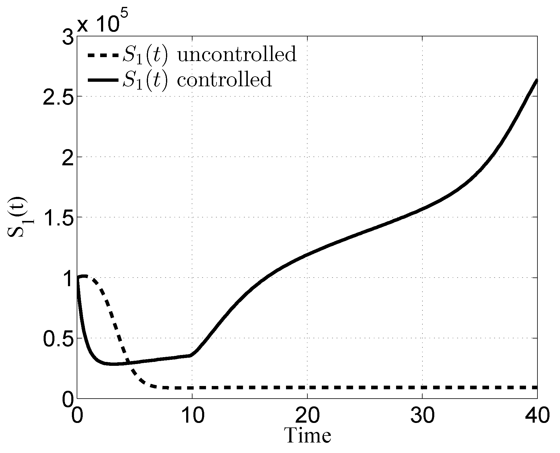
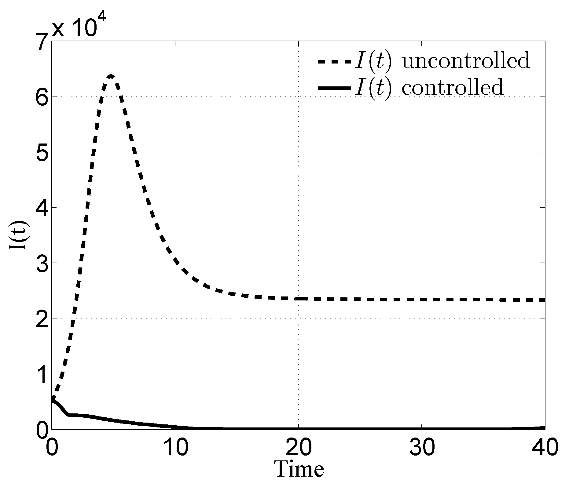
In Figure 2, Figure 3, Figure 4, Figure 5 and Figure 6 the controlled state variables are shown along with the free evolutions for comparative purpose. It could be appreciated that the number of susceptible subjects increases, Figure 2 and Figure 3, thanks to the optimal combination of the control effort $u_1$ and $u_2$ that concur in avoiding incautious behaviours of susceptible subjects and having a fast diagnosis, thus again avoiding dangerous contacts. The control $u_2$ concurred in decreasing the number of infected subjects $I\left(t\right)$, Figure 4, since it was devoted to help the subjects to discover, as soon as possible, the illness and if they belong to the $P\left(t\right)$ or $A\left(t\right)$ patients.

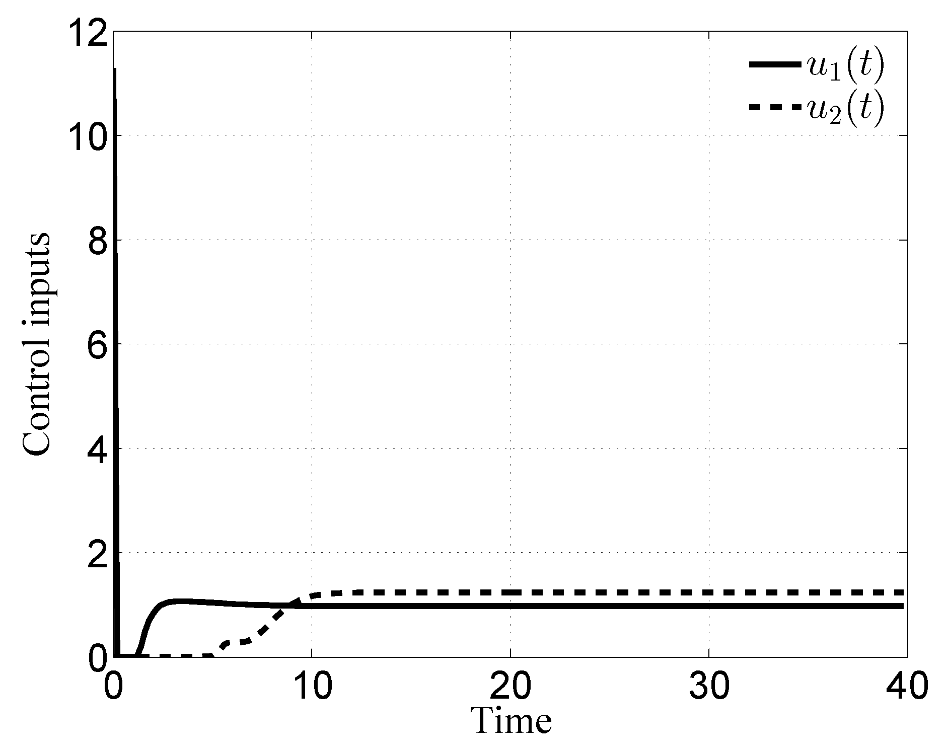
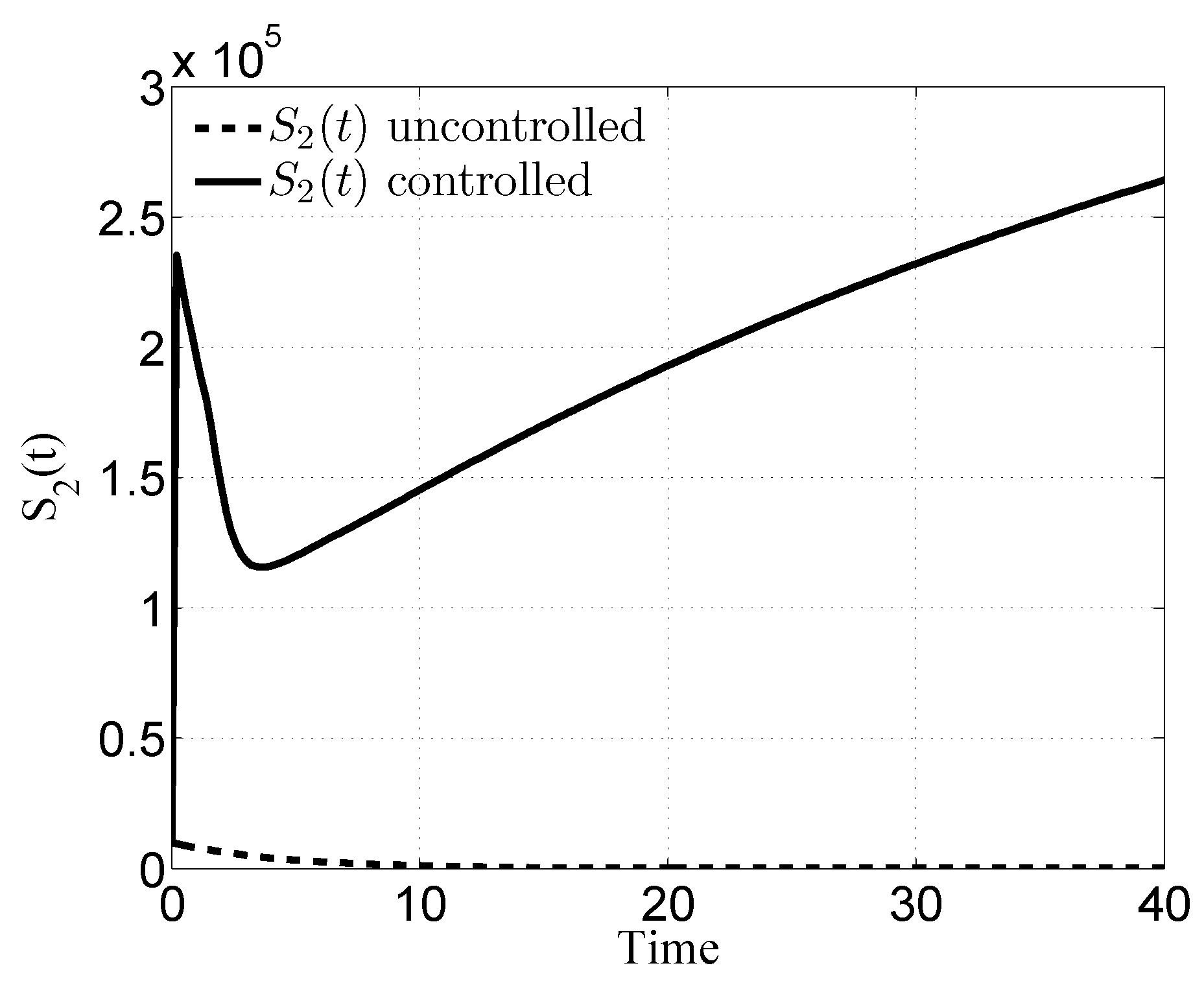
The number of subjects in the pre-AIDS condition $P\left(t\right)$ at the beginning increases (but less than in the case of absence of control) and then it significantly decreases almost to zero, Figure 5. The same happened for $A\left(t\right)$: while in the non-controlled condition it goes to a value of more than 20,000 subjects, with a controlled situation it shows a maximum valued reduced of about one order of magnitude and then definitely decreases to almost zero, Figure 6. It was interesting to note that these results did not require the third control action, as can be observed in Figure 7; it confirms the importance of the optimal combination of the prevention actions $u_1\left(t\right)$ and $u_2\left(t\right)$. In the case considered, the medication seemed not useful to the total reduction of the (weighted) sum of both $P\left(t\right)$ and $A\left(t\right)$. This was actually true for the cynical reason that there is a higher mortality in $A\left(t\right)$ than in $P\left(t\right)$ and then any action which keeps subjects in $P\left(t\right)$ is in contrast with the minimization requirements. This latter consideration suggested to neglect the third control in the other cases considered below, so simplifying notations and expressions without lost of effectiveness.

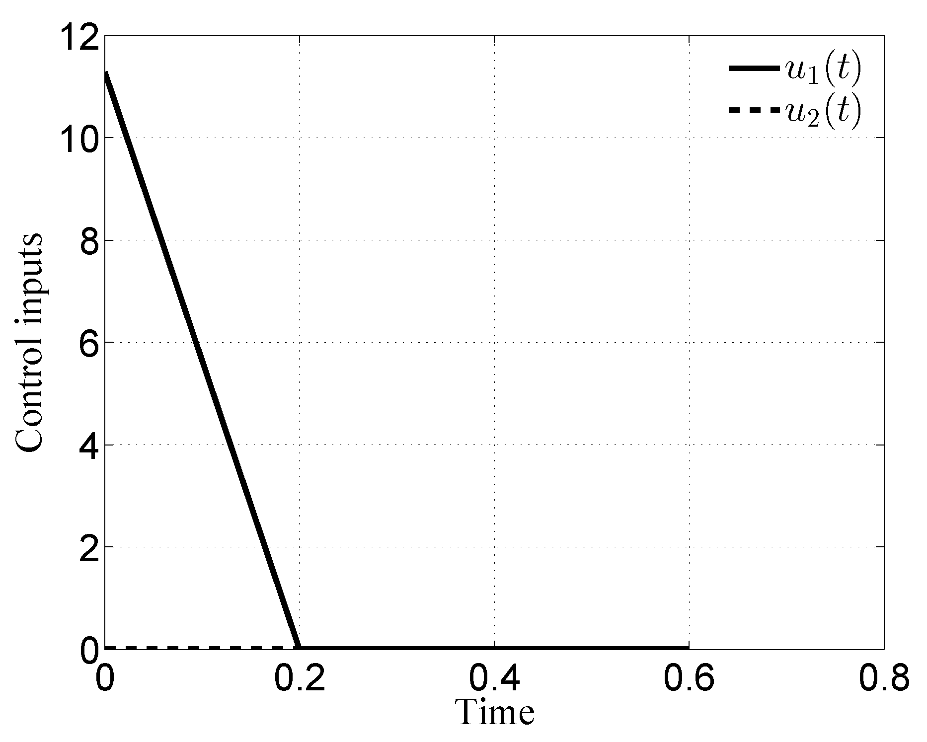
It is interesting to observe from Figure 7 that this kind of control limitation brings to a greater importance of the informative campaign, the first control $u_1\left(t\right)$, at the beginning of the intervention, while the test campaign, the second control $u_2\left(t\right)$, becomes more effective in the second part of time action. The fact that their sum appears in the cost index justifies this sort of switching between each other, solution that avoid the more expensive case of contemporary, and then summed, actions.

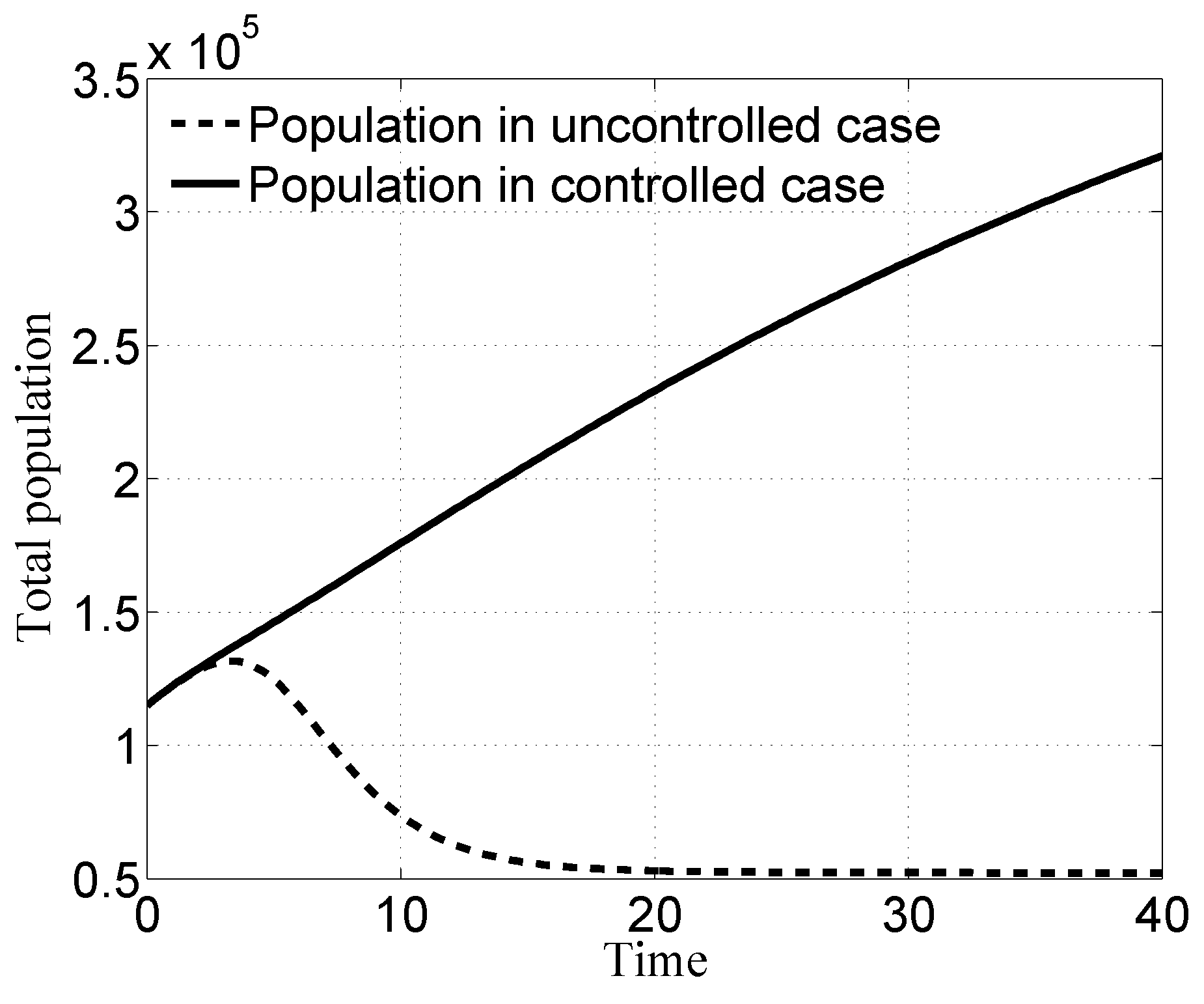
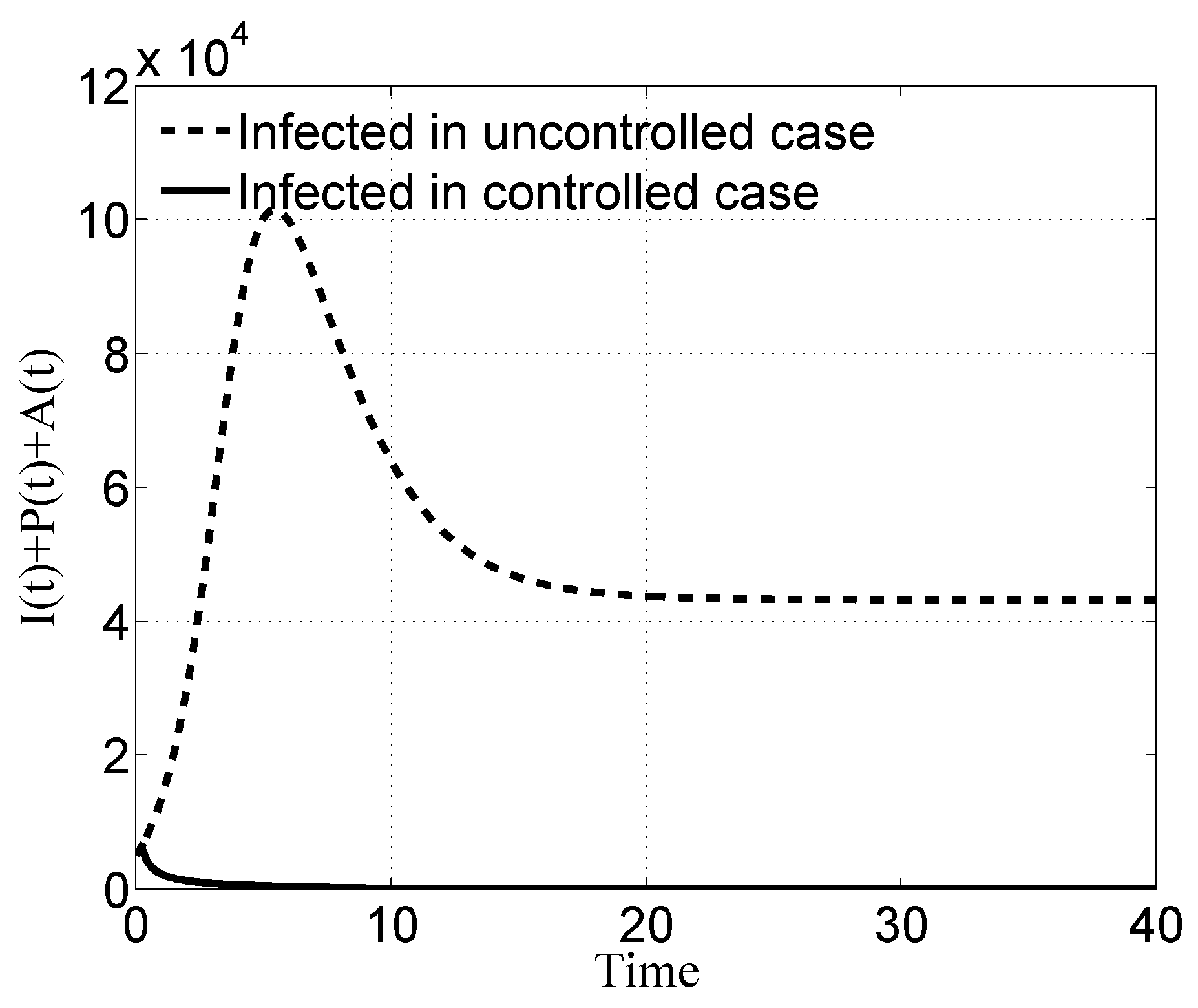
The overall effectiveness of the optimal control action is well evidenced from Figure 8, where the total number of infected people I, P and A are depicted comparing the controlled and the uncontrolled cases, showing a sensible reduction of the infection spread; the effectiveness of the control action results more evident once Figure 8 is related with the time history of the total population in Figure 9, where the controlled case shows a population growth with respect to a quite low state steady endemic case.

3.2. Case ii

In this case the instantaneous constraint on the control actions were formulated so that the limitation involves the sum of the controls. As previously motivated, from here on the third control $u_3\left(t\right)$, the therapy for the P subjects was considered no more. The constraints (38),

$$\begin{array}{ccc}\hfill u_1\left(t\right)& \ge & 0\hfill \\ \hfill u_2\left(t\right)& \ge & 0\hfill \\ \hfill u_1\left(t\right)+u_2\left(t\right)& \le & U\hfill \end{array}$$

were used. Since for the case $i.$ an upper bound equal to one has been assumed for each control, in this case the choice $U=U_1+U_2=2$ is performed to test how the optimal solution divides the maximum action between the two controls to compare the results with the previous case in which the division was performed a priori.

The results were almost similar to the ones of the previous case for what concerns the state evolution. The number of susceptible subjects, the not infected ones, increased, Figure 10 and Figure 11, while, at the same time, the unaware infected subjects $I\left(t\right)$, as well as the diagnosed ones $P\left(t\right)$ and $A\left(t\right)$ decreased; their transient evolution is reported in Figure 12. Differences can be best appreciated in the time evolution of the uninfected people, comparing Figure 2 with Figure 10 and Figure 3 with Figure 11, observing that their number increases. The reason for such a difference can be found in the controls actions, Figure 13. The division of the time interval between the two controls shows almost the same structure as in Figure 7; the difference is in the fact that each control, when mostly active, used all or almost all the available resources while the other control is zero or quite low. In particular, the importance of an initial action of the informative campaign was evidenced once again, while the tests become more important in the second part of the intervention. So, the same switching–like behaviour of the previous case is present also here.

Also in this case, the overall effectiveness of the optimal control action is well evidenced from Figure 14, where the total number of infected people I, P and A is depicted along with the corresponding uncontrolled evolution, and from Figure 15, where the time history of the total population is reported. The shapes are very similar to the case $i.$.

3.3. Case iii

The constraints on the resources considered in this Case are formulated as a total budget for each control, leaving to the optimal solution the best choice for the distribution of this amount of resources along the time. The control constraints are the ones in (68)

$${\int }_0^{t_f}{u}_i\left(t\right)dt=U_i,i=1,2$$

(97)

along with (71)

$$u_i\left(t\right)\ge 0,i=1,2$$

(98)

The control $u_3\left(t\right)$ is neglected once again. The numerical choice for $U_i$ is here performed letting each control use a total amount of resources equivalent to the maximum value they were able to use in the previous cases, computed as the upper bounds of case $i.$ times the time interval of control action, yielding to $U_1=U_2=40$.

To illustrate the differences between this case and the previous ones it may be useful to start analysing the control actions reported in Figure 16 and divided into Figure 17, for the very first time interval, and Figure 18, for the remaining part, in order to put better in evidence the impulsive–like behaviour of the first control $u_1\left(t\right)$ clearly visible in Figure 17. This result was perfectly in line with what observed in Case $i.$ and Case $ii.$ about the importance, in the initial time instants, of the control $u_1\left(t\right)$: the higher is the maximum value allowed, the higher the amplitude it reached, compatibly with all the other constraints.

After this characteristic behaviour in the initial time, a constant action of both the control, Figure 18, with $u_2\left(t\right)$ a little bit higher than $u_1\left(t\right)$, also due to the fact that the first control has already used some of the resources at $t=0$, so having a lowed amount with respect to the second control.

The effects of the strong initial action of the first control can be observed in Figure 19 and Figure 20, where a faster change of the time evolutions of $S_1\left(t\right)$ (Figure 19) and $S_2\left(t\right)$ (Figure 20) in the first quarter of the time interval are visible, being these two state variables the ones more directly affected by the first control.

The effects of the long high action of the second control are more visible in the Figure 21, where the transients of the evolutions of the infected individuals $I\left(t\right)$, $P\left(t\right)$ and $A\left(t\right)$ are reported: shorter transients as well as lower values of infected people in the first transients, in the peak values and in the steady state behaviours are evident.

The same positive effects can be found in Figure 22, the time history of the total infected individuals, and in Figure 23, the time history of the total population.

3.4. Case iv

In this last case, a constraint like the one adopted in the previous case $iii.$ is considered but with the difference that the total budget available is common for both the controls. This means that the optimal control was formulated so that the optimal solution had to distribute the resources between the controls and over the time action. The expressions are the ones in (85) and (71),

$${\int }_0^{t_f}\left(u_1\left(t\right)+u_2\left(t\right)\right)dt=U$$

(99)

$$u_i\left(t\right)\ge 0,i=1,2.$$

(100)

The maximum budget U is numerically assumed equal to the sum of the budgets assigned to each of the controls in the previous case, so that $U=80$.

This case can be compared with the previous one. Starting again from the control actions reported in Figure 24 and, more usefully, in Figure 25, with the very first time interval, and Figure 26, with the remaining part, it can be noticed that the structure is almost the same as Case $iii.$ The differences can be motivated on the basis of the results discussed for the cases $i.$ and $ii.$ The impulsive-like behaviour of $u_1\left(t\right)$ was confirmed, but since the resources must be shared over the time, differently from the previous case the greater importance of $u_2\left(t\right)$ after the initial action of $u_1\left(t\right)$ brings to the fact that after the initial impulse, the first control is almost no more requested to act, with values around 0.1 starting from about $t=1$, while the action of $u_2\left(t\right)$ increases and then it uses about the same resources used in the previous case by the sum of the two controls. Once again, the importance of the first control in the initial time as well as the higher relevance of the second control during the longer part of the final time action are confirmed.

The effects on the state behaviour were a confirmed fast change of $S_1\left(t\right)$ (Figure 27) and $S_2\left(t\right)$ (Figure 28) in the first part of the time interval, due to the initial high peak of $u_1\left(t\right)$ which mainly affects these two state variables, as long as a stronger effect of $u_2\left(t\right)$ on the infected individuals I, P and A, Figure 29 for the transient part of the evolution, which is evidenced by a faster decrement of their quantities and by lower steady state values.

Once again, the overall positive effects can be found in Figure 30, the time history of the total infected individuals, and in Figure 31, the time history of the total population.

4. Discussion

The problem of an effective resources allocation is common in a large variety of applications. Four cases have been here addressed combining instantaneous bounds on the control and total amount of resources over the total time control with the separation of the constraints on each control and the common constraint on all the controls together.

The particular results for the model considered show that there is a difference in the effectiveness of each control over different time interval, being more important one control, $u_1\left(t\right)$, in the initial time interval, becoming more important the other one, $u_2\left(t\right)$, in the second part of the control action. Moreover, the intensity of the actions, depending on the structure of the bounds, results higher in the most effective instants when the allocation between the two controls is left to the optimal solution, as in the Case $iv.$ with respect to Case $iii.$ or Case $ii.$ with respect to Case $i.$

This result can be generalized in the sense that the solution of one optimal control problem can allocate the resources, among the controls and over the time action, in a better way than it could be possible assuming a priori choices.

References

- Guo, J.; Mu, B.; Wang, L.Y.; Yin, G.; Xu, L. Decision-Based System Identification and Adaptive Resource Allocation. IEEE Trans. Autom. Control 2017, 62, 2166–2179. [Google Scholar] [CrossRef]
- Li, J.; Han, Y. Optimal Resource Allocation for Packet Delay Minimization in Multi-Layer UAV Networks. IEEE Commun. Lett. 2017, 21, 580–583. [Google Scholar] [CrossRef]
- Xianglan, W.; Jun, Z. Optimal allocation of resources in the material production sector and human capital sector. In Proceedings of the 2011 IEEE 2nd International Conference on Computing, Control and Industrial Engineering, Wuhan, China, 20–21 August 2011. [Google Scholar]
- Winz, I.; Brierley, G.; Trowsdale, S. The Use of System Dynamics Simulation in Water Resources Management. Water Resour. Manag. 2009, 23, 1301–1323. [Google Scholar] [CrossRef]
- Viswanadham, N.; Balaji, K. Resource allocation for healthcare organizations. In Proceedings of the 2011 IEEE International Conference on Automation Science and Engineering, Trieste, Italy, 24–27 August 2011. [Google Scholar]
- He, Z.L.; Li, J.; Nie, L.; Zhao, Z. Nonlinear state-dependent feedback control strategy in the SIR epidemic model with resource limitation. Adv. Differ. Equ. 2017, 209, 1–18. [Google Scholar] [CrossRef]
- Denysiuk, R.; Torres, C.S.D. Multiobjective optimization to a TB-HIV/AIDS coinfection optimal control problem. Comput. Appl. Math. 2018, 37, 2112–2128. [Google Scholar] [CrossRef]
- Nareshn, R.; Tripathi, A.; Sharma, D. Modeling and analysis of the spread of AIDS epidemic with immigration of HIV infectives. Math. Comput. Modell. 2009, 48, 800–892. [Google Scholar]
- Wodarz, D.; Nowak, M. Specific therapy regimes could lead to long-term immunological control of HIV. Proc. Natl. Acad. Sci. USA 1999, 96, 14464–14469. [Google Scholar] [CrossRef] [PubMed] [Green Version]
- Chang, H.; Astolfi, A. Control of HIV infection dynamics. IEEE Control Syst. 2008, 28, 28–39. [Google Scholar]
- Pinto, C.; Rocha, D. A new mathematical model for co-infection of malaria and HIV. In Proceedings of the 4th IEEE International Conference on Nonlinear Science and Complexity, Budapest, Hungary, 6–11 August 2012. [Google Scholar]
- Di Giamberardino, P.; Compagnucci, L.; Giorgi, C.D.; Iacoviello, D. A new model of the HIV/AIDS infection diffusion and analysis of the intervention effects. In Proceedings of the 25th Mediterranean Conference on Control and Automation, Valletta, Malta, 3–6 July 2017. [Google Scholar]
- Di Giamberardino, P.; Compagnucci, L.; Giorgi, C.D.; Iacoviello, D. Modeling the effects of prevention and early diagnosis on HIV/AIDS infection diffusion. IEEE Trans. Syst. Man Cybern. Syst. 2017, 99, 1–12. [Google Scholar] [CrossRef]
- Di Giamberardino, P.; Iacoviello, D. An Optimal Control Problem Formulation for a State Dependent Resource Allocation Strategy. In Proceedings of the International Conference on Informatics in Control, Automation and Robotics, Madrid, Spain, 26–28 July 2017. [Google Scholar]
- Di Giamberardino, P.; Iacoviello, D. Optimal Control of SIR Epidemic Model with State Dependent Switching Cost Index. Biomed. Signal Process. Control 2017, 31, 377–380. [Google Scholar] [CrossRef]
- Rutherford, A.R.; Ramadanovic, B.; Michelow, W.; Marshall, B.D.L.; Small, W.; Deering, K.; Vasarhelyi, K. Control of an HIV epidemic among injection drug users: simulations modeling on complex networks. In Proceedings of the 2016 Winter Simulations Conference, Washington, DC, USA, 11–14 December 2016. [Google Scholar]
- Di Giamberardino, P.; Iacoviello, D. Optimal Control to reduce the HIV/AIDS spread. In Proceedings of the 22nd International Conference on System Theory, Control and Computing (ICSTCC), Sinaia, Romania, 10–12 October 2018. [Google Scholar]
- Bakare, E.A.; Nwagwo, A.; Danso-Addo, E. Optimal control analyis of an SIR epidemic model with constant recruitment. Int. J. Appl. Math. Res. 2014, 3, 273–285. [Google Scholar] [CrossRef]
- Lin, F.; Muthuraman, K.; Lawley, M. Optimal control theory approach to non-pharmaceutical interventions. Int. J. Appl. Math. Res. 2010, 10, 1–13. [Google Scholar] [CrossRef] [PubMed]
- Iacoviello, D.; Stasio, N. Optimal control for SIRC epidemic outbreak. Comput. Methods Programs Biomed. 2013, 110, 333–342. [Google Scholar] [CrossRef] [PubMed]
- Owuor, O.N.; Johannes, M.; Kibet, M.S. Optimal vaccination strategies in an SIR epidemic model with time scales. Appl. Math. 2013, 4, 37454. [Google Scholar] [CrossRef]
- Anderson, B.D.O.; Moore, J.B. Optimal Control—Linear Quadratic Methods; Prcntice-Hall: Englewood Cliffs, NJ, USA, 1989. [Google Scholar]
- Fletcher, R. Practical Methods of Optimization; Wiley: New York, NY, USA, 1987. [Google Scholar]
- Gill, P.; Murray, W.; Wright, M.H. Practical Optimization; Academic Press: London, UK, 1981. [Google Scholar]
- Battiti, R. First and second order methods for learning: between steepest descent and Newton’s method. Neural Comput. 1992, 4, 141–166. [Google Scholar] [CrossRef]
Figure 1.
Block diagram of the considered model.
Figure 2.
Case i: time evolution of the subjects with and without optimal control actions.
Figure 3.
Figure 4.
Case i [17]: time evolution of the subjects with and without optimal control actions.
Figure 5.
Figure 6.
Figure 7.
Case i [17]: optimal controls.
Figure 8.
Case i [17]: time evolution of the total number of infected, with and without the control actions.
Figure 9.
Case i [17]: time evolution of all the population, with and without the control actions.
Figure 10.
Case ii: time evolution of the subjects with and without optimal control actions.
Figure 11.
Figure 12.
Case ii: time evolution of the transient for infected , and subjects under optimal control actions.
Figure 13.
Case ii: optimal controls.
Figure 14.
Case ii: time evolution of the total number of infected, with and without the control actions.
Figure 15.
Case ii: time evolution of all the population, with and without the control actions.
Figure 16.
Case iii: optimal controls.
Figure 17.
Case iii: optimal controls in the very first time of intervention .
Figure 18.
Case iii: optimal controls after the the very first time of intervention .
Figure 19.
Case iii: time evolution of the subjects with and without optimal control actions.
Figure 20.
Figure 21.
Case iii: time evolution of the transient for infected , and subjects under optimal control actions.
Figure 22.
Case iii: time evolution of the total number of infected, with and without the control actions.
Figure 23.
Case iii: time evolution of all the population, with and without the control actions.
Figure 24.
Case iv: optimal controls.
Figure 25.
Case iv: optimal controls in the very first time of intervention .
Figure 26.
Case iv: optimal controls after the the very first time of intervention .
Figure 27.
Case iv: time evolution of the subjects with and without optimal control actions.
Figure 28.
Figure 29.
Case iv: time evolution of the transient for infected , and subjects under optimal control actions.
Figure 30.
Case iv: time evolution of the total number of infected, with and without the control actions.
Figure 31.
Case iv: time evolution of all the population, with and without the control actions.
© 2019 by the authors. Licensee MDPI, Basel, Switzerland. This article is an open access article distributed under the terms and conditions of the Creative Commons Attribution (CC BY) license (http://creativecommons.org/licenses/by/4.0/).
Share and Cite
MDPI and ACS Style
Di Giamberardino, P.; Iacoviello, D. Optimal Control of Virus Spread under Different Conditions of Resources Limitations. Information 2019, 10, 214. https://doi.org/10.3390/info10060214
AMA Style
Di Giamberardino P, Iacoviello D. Optimal Control of Virus Spread under Different Conditions of Resources Limitations. Information. 2019; 10(6):214. https://doi.org/10.3390/info10060214
Chicago/Turabian StyleDi Giamberardino, Paolo, and Daniela Iacoviello. 2019. "Optimal Control of Virus Spread under Different Conditions of Resources Limitations" Information 10, no. 6: 214. https://doi.org/10.3390/info10060214
Note that from the first issue of 2016, this journal uses article numbers instead of page numbers. See further details here.