
Ship Classification Based on Improved Convolutional Neural Network Architecture for Intelligent Transport Systems


School of Information Engineering, Wuhan University of Technology, Wuhan 430081, China
*
Author to whom correspondence should be addressed.
Information 2021, 12(8), 302; https://doi.org/10.3390/info12080302
Submission received: 3 July 2021
/
Revised: 18 July 2021
/
Accepted: 27 July 2021
/
Published: 28 July 2021
(This article belongs to the Special Issue New Trends and Challenges in Intelligent Transportation Systems Optimisation, Modeling and Security)
Abstract
:In recent years, deep learning has been used in various applications including the classification of ship targets in inland waterways for enhancing intelligent transport systems. Various researchers introduced different classification algorithms, but they still face the problems of low accuracy and misclassification of other target objects. Hence, there is still a need to do more research on solving the above problems to prevent collisions in inland waterways. In this paper, we introduce a new convolutional neural network classification algorithm capable of classifying five classes of ships, including cargo, military, carrier, cruise and tanker ships, in inland waterways. The game of deep learning ship dataset, which is a public dataset originating from Kaggle, has been used for all experiments. Initially, the five pretrained models (which are AlexNet, VGG, Inception V3 ResNet and GoogleNet) were used on the dataset in order to select the best model based on its performance. Resnet-152 achieved the best model with an accuracy of 90.56%, and AlexNet achieved a lower accuracy of 63.42%. Furthermore, Resnet-152 was improved by adding a classification block which contained two fully connected layers, followed by ReLu for learning new characteristics of our training dataset and a dropout layer to resolve the problem of a diminishing gradient. For generalization, our proposed method was also tested on the MARVEL dataset, which consists of more than 10,000 images and 26 categories of ships. Furthermore, the proposed algorithm was compared with existing algorithms and obtained high performance compared with the others, with an accuracy of 95.8%, precision of 95.83%, recall of 95.80%, specificity of 95.07% and F1 score of 95.81%.
1. Introduction
The purpose of ship classification is to identify various types of ships as accurately as possible, which is of great significance for monitoring the rights and interests of maritime traffic and improving coastal defense early warnings. With the improvement of all kinds of imaging technology, the ship classification method of imaging technology has become the mainstream method of ship target classification and recognition. From the data, the ship image can be roughly divided into the radar image, satellite remote-sensing image, infrared image and visible light image. The most widely used radar imaging technology is synthetic aperture radar (SAR). The advantages of SAR imaging are a wide monitoring range, short observation period and all-weather monitoring. On the other hand, the price of using radar is being vulnerable to other electromagnetic interference. Moreover, the captured ship targets only account for a few parts of the whole image. The classification method for radar images is only suitable for larger targets. The classification effect for a boat with a long distance is better than that for optical remote-sensing satellite imaging, which is easily affected by changes in ocean weather and light, making it hard to do real-time monitoring for a long time. Infrared imaging can provide rich target information and target backgrounds obtained at night or in the case of insufficient light, and it has a strong anti-jamming ability. However, infrared imaging is affected by the weather, temperature and other factors. On the sea surface, the influence of waves, clouds and other interference will greatly affect the accuracy of the image. Thus, infrared imaging cannot provide rich color information if the image quality is low. The visible light image contains gray information for multiple bands, and the image quality improves steadily, which makes the target features easier to be found and extracted. For the problem of ship classification, the actual system can get a variety of images. This can be solved using fusion methods that can produce high-resolution multispectral images from a high-resolution panchromatic image and low-resolution multispectral images [1,2].
Several traditional algorithms were suggested by Rainey et al. [3] for extraction and identification of the ship image. These include LBP, hog and sift and also classifiers such as the nearest neighbor algorithm and SVM. Arguedas [4] used LBP features to remove texture features from ship images to classify ships. Parameswarans et al. [5] used the bag of words model in classifying texts and used the bag of words model in ship classification. A two-stage ship recognition technique based on structural features was proposed. The method can effectively distinguish ships and cargo ships according to the ship image. Leclerc et al. [6] proposed a commercial ship classification algorithm based on structural feature analysis which can distinguish the features of density estimation, the position of the ship’s integral principal axis and the proportion of integral quantity of the left, middle and right parts. Through a synchronous experiment in the East China Sea experimental area, it was proven that the average classification accuracy of COSMO-SkyMed image quotient method was 89.94%. Liang Jinxiong et al. [7] suggested the use of a BP neural network to classify six infrared images. After pre-processing the images, the Hu invariant moment, edge image and perimeter area ratio were selected, and the accuracy of the four-layer BP neural network was about 84%. The traditional ship image classification method is based on the expert system, which can recognize the ship according to the ship type and lacks good generalization performance. Therefore, ship classification accuracy needs to be enhanced. With the rapid development of edge metering and word learning, convolutional neural networks have become a research hotspot in the field of image classification. Rainey et al. [8] created and acquired a convolutional neural network to recognize ships from satellite images and achieved good results. Liu et al. [9] proposed an improved residual network to detect and classify remote-sensing ship images which is prone to overfitting due to a small dataset. Khellal et al. [10] proposed using an extreme learning network to recognize a ship’s infrared image. This method is suitable for infrared recognition systems. After using extreme learning features, it also needs to use extreme learning machines based on integration for classification. Therefore, this method proposes a CNN model with multi-resolution input. The performance of the proposed method was evaluated with TerraSAR-X images which were composed of five maritime categories. The classification effect was different, but how the change in the image resolution affected the internal activation of the CNN was still unclear from the test. Chen Xingwei [11] proposed a method for extracting multiple ship classification features such as the contrast, entropy, energy and inverse moment features to obtain a feature vector set and taking the feature vector set as the input of the deep learning algorithm to create a ship classifier model. The classification accuracy of the self-built dataset was more than 90%. H. Zhu et al. [12] proposed an all new classification architecture for SAR images of ships via deep learning. The classification architecture attained an accuracy of 99.24%. Liu et al. [13] proposed the latest target classification algorithm, improved Inception V3 and center loss convention neural network (IICL-CNN), established on a well-established network to improve the accuracy of ambiguous targets. It performed best with ambiguous ship targets compared with the original Inception V3 model. Pedroche et al. [14] proposed a data preparation process for real-world kinetic data management and the detection of fishing vessels. These features are intended for modeling ship behavior, but since they do not include context-related information, the classification can be applied in other scenarios. Li et al. [15] indicated ship classification methods for the practical testing of satellite images and specified the respective techniques and statistics for the extraction of features. Qiu et al. [16] proposed a dual double seaport classification system based on multilayer complex facility fusion. It obtained high accuracy, but it had the drawbacks of other features not being extracted and being time-consuming.
Until recently, more researchers have still been researching how to obtain a good classification algorithm. All the existing studies have achieved good classification results, but it is important to perform more research on comparison analysis of classification algorithms using convolutional neural networks in a visible light image dataset and selecting which one is suitable while also introducing a new classification algorithm which can improve the accuracy of predicting ships in inland waterways so as to avoid collisions which are likely to occur. To solve the above limitation, the following contributions have been made for the proposed classification system. First, a new convolutional neural network architecture has been employed which consists of two fully connected layers followed by ReLu and drop out to improve the accuracy of ship classification systems. Secondly, to ensure the generalization of the network, the improved CNN has been tested on the MARVEL dataset, which consists of more than 10,000 images and 26 categories of ships. Finally, a comparison has been performed between the proposed ship classification systems and other existing classification algorithms.
2. Materials and Methods
2.1. Convolutional Neural Network Structure
A CNN has three notable features, namely weight sharing, a local connection and subsampling in time and space. Unlike a simple BP neural network that uses all fully connected layers, a CNN includes many different types, such as convolutional layers, pooling layers and fully connected layers. These layers are used to better extract target features while reducing the model parameters. At the same time, the advantage is that a CNN does not require artificial design features, which is also the reason why it is widely studied. In this section, a variety of classic CNN models are used to classify the ships dataset.
2.2. Classic CNN Model
In order to determine the overall structure and complexity of the feature extraction network in the ship target detection algorithm, in this section, we selected AlexNet, VGG-16, Inception V3, ResNet-18, ResNet-34, ResNet-50, ResNet-101,ResNet-152 and GoogleNet from the common convolutional neural networks [17], and various experimental comparisons have been performed to obtain the best classification algorithm.
- (a)
- AlexNet
AlexNet was researched and designed by AI godfather Hinton and his student Alex Krizhevsky, and it won the championship in the ILSVRC-2012 image classification competition. The task index was 10 percentage points higher than the second place winner. It contains 5 convolutional layers, two fully connected layers and softmax as the last layer, which helps with prediction. AlexNet’s new ideas include abandoning sigmoid and tanh and adopting the ReLU activation function to make the network converge faster. ReLU is already the activation function used by most networks today. The local response normalization layer (local response normalization (LRN)) prevents overfitting and enhances the generalization ability of the network, but later researchers rarely used it. AlexNet was also one of the first networks to adopt GPU acceleration, which promoted the development of deep networks.
- (b)
- VGG-16
The VGG-16 network has the basic structure of downsampling with the largest pooling layer after multiple convolutional layers with a convolution kernel size of 3 × 3. VGG-16 is one of the widely used levels in VGGNet’s multi-level network. After going through multiple structures composed of a convolutional layer and pooling layer, the VGG-16 network uses all the output of the last pooling layer as the input of the fully connected layer in the network and passes through three consecutive fully connected layers to give the confidence of each category. Since VGG-16 has three fully connected layers containing a large number of parameters, the model will take up more memory and consume more computing resources.
- (c)
- ResNet-152
Before the residual network (ResNet) came out, it was difficult for researchers to solve the problem that increasing the depth of the neural network would lead to gradient dispersion, gradient explosion and network degradation, so it was impossible to build a deeper network. However, in theory, because a CNN extracts features from a low-level to high-level process, more layers, to a certain extent, means that features containing more information can be extracted, which has a direct benefit for the overall performance. Gradient dispersion and explosion can be significantly improved through standard parameter initialization and proper regularization. He Kaiming and others believe that network degradation is due to the fact that the optimal depth of the network may only be the first segment of the present, and the parameters of the last segment make it difficult to learn the identity transformation. In order to learn the identity transformation more easily, the identity mapping [18] was introduced, the structure of which is shown in Figure 1.
In the residual structure shown in Figure 1, if the input is x, the weight layer is a 3 × 3 convolutional layer and the mapping learned through multiple multilayer networks containing parameters in the structure is f(x), then the output of the residual structure is f(x) + x. In the network, assuming that the mth through Mth layers are composed of such multiple continuous residual structures, the forward propagation process of this part of the network is shown in Equation (1):
where is the output of these continuous residual structures, is the input of the first layer, is the parameter of the ith layer from the mth layer to the Mth layer and is the input of the ith layer.
When performing backpropagation, according to the chain rule, the calculation process of the gradient of the first layer in the network is shown in Equation (2):
It can be found from Equation (2) that the gradient of the first layer contained a partial derivative term directly derived from the error of the layer. Even if the gradient of the latter layer was extremely small, the gradient would not disappear in this layer.
- (d)
- InceptionV3
Google’s Inception series models from V1 to V3 start from the width of the model instead of the depth. It is believed that the size of the convolution kernel required for objects of different sizes is also different, so the parallel convolution kernel is adopted. At the same time, the Inception network also performs well in terms of model size and computational efficiency. For example, when using two 3 × 3 convolution kernels instead of a 5 × 5 convolution kernel, the expression ability is not weakened while reducing the number of parameters.
- (e)
- GoogleNet
GoogleNet is a 22-layer deep convolutional neural network that is a variant of the Inception network, a deep convolutional neural network developed by researchers at Google. It was introduced to provide more efficiency in classification and detection. It is currently being used in classification techniques.
3. Classification Dataset and Hyperparameter Setting
3.1. Dataset Description
The dataset used in this experiment is public game of deep learning ship dataset which can be found on Kaggle [19]. The dataset consisted of five categories of ships: cargo, military, cruise, carrier and tanker ships, better distinguishing the classification capabilities of different neural networks for inland ships and thus reflecting the impact of inland rivers when different classification networks were adjusted as the backbone network. The images of the ships were taken from different directions, in different weather conditions, at different shooting distances and angles and from different international and offshore harbors. The dataset consists of 8932 images, and there exist both RGB images and grayscale images with different image pixel sizes. In this dataset, the number of samples of all types is more than 800, which can meet the needs of model training and testing. The dataset was divided at a ratio of 70:30, with 70% for training and 30% for testing. Figure 2 below shows sample images existing in the dataset.
3.2. Evaluation Indicators
Evaluation indicators are indicators which are used to measure the network performance of the model. In this chapter, for evaluation of the classification algorithm, we used these indicators: accuracy, precision, recall and specificity. Accuracy measured how accurate the model was, while precision measured how accurately the ships were classified and recall measured how well the negative samples were detected. Specificity measured how different classes of ships were classified. The F1 score was the addition of precision and recall. There mathematical formulations are given in the equations below:
where in Equations (3)–(5), represents the true positive number of accurately classified ships, represents false positives (meaning incorrectly classified ships), means false negative (i.e., incorrect or misclassified ships), represents true negative and represents false positive. The sum of the samples for and is all the samples predicted to be positive, and the sum total of and is all samples labeled positive.
3.3. Experiment Set-up and Process
- (a)
- Image pre-processing
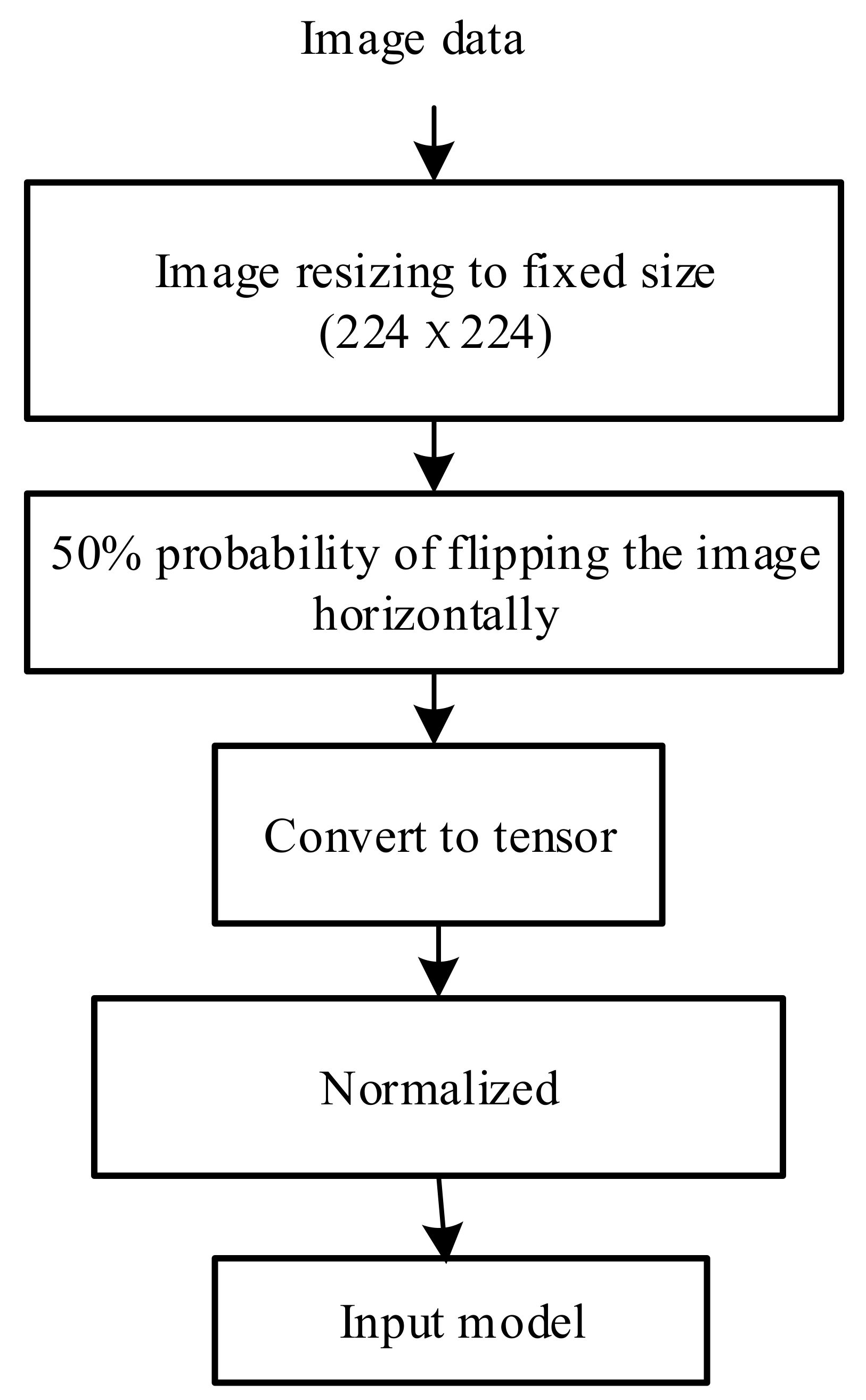
When training deep convolutional neural networks, proper pre-processing of the images can effectively speed up the convergence speed during training. The pre-processing methods used in this chapter are shown in Figure 3.
The normalization formula is shown in Equation (7), where the image channel is represented by , the mean is represented by and the standard deviation is represented by :
- (b)
- Parameter initialization
To speed up the training process, the network in this experiment was initialized with the parameters of the ImageNet pretraining network. Because ImageNet and our dataset had different categories, the last layer of the network needed to be adjusted. The pretraining weights of this layer could not be used. The Kaiming Norm [20] method was used to initialize this layer.
This initialization method initialized the parameters of the convolutional layer with a random value of a normal distribution with a mean value of 0 and a standard deviation of σ. The value of the standard deviation σ is shown in Equation (8):
In the formula, the number of input layer features is represented by .
- (c)
- Hyperparameter settings
The hyperparameter settings of each network in the experiment are shown in Table 1.
During the experiment, the training set’s accuracy was recorded for every epoch, and the test set’s accuracy was recorded when training was over. The entire experiment was run in Google Colab. Initially, the present pretrained AlexNet [21], VGG [22], Inception-V3 [23], ResNet [24] and GoogleNet [25] were adjusted to the game of deep learning ship dataset for ultimate network performance in the suggested real-time ship application. With regard to various models’ performance, the best-performing model was chosen to improve the network classification accuracy. The models were adjusted according to the classes found in the public dataset. These network models were trained in the PyTorch framework, and the momentum and learning rate were optimized using Adam. The cross-entropy loss function was employed for collecting loss in the entire process, and after each epoch, validation was performed to evaluate learning during network training. As can be seen in Figure 4, the accuracy performance of ResNet-152 was higher compared with AlexNet, VGG, Inception V3 and GoogleNet. The accuracy of ResNet was 90.56%, while the model which acquired low accuracy was AlexNet, which differed by 27.14%. GoogleNet obtained an accuracy of 81.23%, higher than that of VGG and AlexNet. However, the VGG model also acquired 79.28% accuracy, much higher than the AlexNet model. Furthermore, Inception V3 obtained 86.45% accuracy. Through the experiment, it is believed that improving the ResNet model will lead to higher accuracy, and the model can be used for classification.
4. Proposed Method
In order to solve the problems described above for the accuracy of the classification system, we proposed a new classification model. First, based on the pretrained models (AlexNet, VGG, Inception V3, ResNet and GoogleNet), as described above in Section 2.2, the models were fine-tuned with the public dataset we used. Based on their performance, the best model was selected in order to further adjust the performance for high accuracy in classifying ships in inland river waterways. After selecting the best model, the model was adjusted, and classification was conducted based on the modification of the network. The overall process is shown in Figure 5 below.
4.1. Network Adjustment
The architecture of ResNet 152 had 152 layers of depth. This was accomplished with the replacement of a three-layer bottleneck block for every two layers of ResNet [21]. The network input layer took an RGB color image of 224 × 224 pixels. Figure 5 shows that the provided method’s structure included 64 convolution kernels, 7 × 7, with a first layer step of 2 and a max-pool layer of 3 × 3 × 2.
For the first convention layer, stride 2 was employed. In addition, in the preceding layers (i.e., from layer 2 to layer 5), three-layer bottleneck blocks were used. Convolution block 2 consisted of 128 filters, block 3 had 256 filters, block 4 had 1024 filters and block 5 had 2048 filters. The next layer was the average pooling. The last fully connected layer of transfer learning was removed from the network because it was trained for 1000 categories, and we only had 5 categories in our dataset. An additional classification block was used which contained a fully connected (FC) layer with 1024 neurons. This layer was followed by average pooling and a ReLu layer for learning new characteristics of our training dataset. Next, we introduced a dropout layer on the bottom of the network to resolve the problem of a diminishing gradient. A new fully connected layer for five types of classification of ships was added on the basis of the classification block, where every previous layer connected the five output classes by using the softmax function. The learning rates of these new layers were modified so they could learn well the features of our training dataset. With a batch size of 32 and the number of epochs set to 20, training took 8 h.
4.2. Experiment Results and Analysis
The proposed ResNet structure, as mentioned in the previous section, aimed at improving the performance of the network. An additional classification block was used which contained a fully connected (FC) layer with 1024 neurons. This layer was followed by average pooling and a ReLu layer for learning the new characteristics of our training dataset. For enhancing the stability of the network and discovering the best feature extraction vector of the fully connected layers, ResNet with 152 layers was examined using a public ship dataset with several permutations of the vectors of fully linked layers in the proposed classifying block.
Nevertheless, in order to perform transfer learning, the features extracted from previous layers were used to propose the classifying block, gaining the optimum weight and distortion from the input dataset. For training and validation of the proposed classifying algorithm, the same learning and momentum parameters were used. The proposed network of two fully linked (connected layers), higher functional vectors had much greater precision compared with other fully connected layers with lower functional vectors, as can be seen in Table 2. Below the classifying block was the first layer, which was fully related to 2048 features. At the same time, the highly functional, fully connected layers were introduced to the classifying network block. The following phase was evaluation of our network in different depth layers. The accuracy of each layer is shown in Table 3 to verify the network’s performance.
Table 3 shows how the network depth affected the performance of the public ship dataset in terms of accuracy. The performance of the ResNet model was demonstrated to be boosted by increasing the network depth. As a result, ResNet 152 achieved greater accuracy in the overall dataset classes compared with ResNet with fewer depth layers (i.e., Resnet 18, 34, 50 and 101).
The ResNet 152 precise performance matrices are shown in Table 4. It was observed that the classification system failed to fully recognize the cargo and tanker ships, with accuracy percentages of 93.00 and 91.00, respectively, while the carrier, cruise and military classes were accurately classified. The overall accuracy of the classification system was 95.8%. This shows how accurate the proposed classifying system was. In terms of precision, the military, carrier and cruise ships were more than 98% correctly classified, and the lowest precision was obtained by the cargo and tanker classes at 90.29% and 92.86%, respectively. In addition, in terms of specificity, the overall performance obtained was 95.07, which shows that the overall performance of the proposed classification system was good.
4.3. Analysis of Proposed Classification System with the MARVEL Dataset
To ensure the generalization capability of our proposed network, analysis was also conducted on a different public dataset (i.e., the MARVEL data set), where the ships were divided into 26 categories, covering common ship categories which could better distinguish the classification capabilities of different neural networks for inland ships, thus reflecting the impact of inland rivers when different classification networks were adjusted as the backbone network. Five categories (cargo, military, cruise, carrier and tanker) were selected. We randomly selected 140 images in each category to be used as test images for our proposed classification system. The network was not retrained, and only the test images were used for testing the performance of our system. Table 5 shows the classification accuracy of the dataset. It can be observed that even though a different dataset was used, it yielded a greater performance. It can be concluded that the proposed classification algorithm performed best even when used with a different dataset.
From the table, it can be observed that the tanker classification obtained the lowest accuracy (88.65%), and the carrier classification obtained the highest accuracy (96.99%). The overall accuracy was 91.35%, showing that our proposed classification system performed best even with a different dataset. For the other evaluation metrics, precision obtained an overall percentage of 92.47%, while recall’s was 91.35%, specificity’s was 93.33% and the F1 score’s was 91.83%.
4.4. Comparison of Proposed and Existing Methods
The basic goal of classifying ships is to recognize ships as accurately as possible. Human errors may occur if monitoring is conducted manually or when traditional methods are used. A river contains different types of ships, but identifying a certain kind of ship is very difficult. A strong, effective ship classifying network was presented and proven to solve these challenges. This section presents the comparison analysis of the proposed algorithm with different existing techniques. For classifying ships, the use of a public dataset is common for most researchers. Nevertheless, a comparison of various methods used in different research projects is still a remaining unresolved subject. The table below demonstrates our study’s general performance in comparison with the state-of-the-art approaches in the literature.
As stated in Table 6 below, Wang et al. [26] designed an approach to ship categorization using SAR pictures and in situ information. This was based on backscattering-based categorization and ship geometry, and it obtained an accuracy of 82 percent. Zhang et al. [27] demonstrated a deep classification network based on CNN architecture with gnostic field technology. They utilized 0.8 for the CNN output and 0.2 for the gnostic field output. The daily ACC technique’s accuracy was 87.40 percent. For the three classes of ship images, Jiang et al. [28] built their classification architecture based on the dispersion characteristics. Their work was completed with the boat length ratio and an accuracy ratio of 83.33 percent. Gundogdu et al. [29] introduced an SVM-classified CNN model for the extraction of deep features. The total metrics for [29] were 90.93, 90.86, 91.01, 90.84 and 90.93. In another work, ships were recognized and categorized with a raw underwater audio signal by Sheng et al. [30], inspired by the auditory CNN model. In the experiments, the cumulative accuracy classification for 5 ship classes reached 79.2 percent. While Shen et al. [30] had in-depth analysis with a CNN-inspired auditory technique, the five-class classification template yielded worse performance. Leclerc et al. [6] used the method of transfer learning with the Inception V3 network. Various learning rates were obtained to develop a classification network and obtain a total accuracy of 0.889 percent. Our proposed technique surpassed previous studies by utilizing the modified Resnet-152 architecture by adding a classification block with two fully connected layers and testing it on a game of deep learning sea ship dataset. The performance measures are presented in Table 4.
For each class of ship, Table 7 shows the metric performance of the state-of-the-art techniques. Although Wang et al. [26] reported the smallest accuracy in the tanker and cargo classes, Jiang et al. [28] exhibited the lowest accuracy in the carrier class. The military and cruise ship classes were not included. Ucar and Korkmaz [31] obtained high accuracy in the military and cruise ship classes compared with our proposed method with a difference of 0.38%, but for the other classes of ships, it acquired low classification accuracy compared with our proposed method. For overall comparison, our proposed approach performed better than others.
5. Conclusions
This paper introduced a new classification model’s architecture, which is based on improving the ResNet-152 architecture. This improved the performance of the classification model for classifying ships in inland waterways. Initially, the pretrained models used were AlexNet, VGG16, ResNet, Inception V3 and GoogleNet for the game of deep learning sea ship public dataset, which consisted of five classes: cargo, military, carrier, cruise and tanker ships. Based on their performance, the best model was selected for further improvement. The ResNet-152 model performed better compared with the others, with an accuracy of 96.68%. Further improvement was made by adding a new classification block with two fully connected layers followed by ReLu and a dropout Layer. The new proposed method achieved high accuracy compared with the other existing algorithms, with an accuracy of 95.80%. For testing the generalization of the proposed algorithm, it was further tested on the MARVEL public dataset, where it also obtained a good accuracy of 91.35%, proving the accuracy of the proposed method. Lastly, it was compared with other existing algorithms in classifying different classes of ships in inland waterways, and our proposed method achieved better results compared with the others. In future works, the proposed method will be improved in order to classify the ships in different weather conditions using more advanced technology. Additionally, for proper image pre-processing, a comparison of accuracy for noisy and low-contrast images will be used along with the addition of the Jaccard index to compare the accuracy of the classification.
Author Contributions
Conceptualization, methodology and writing—original draft, L.A.L.; methodology, validation and supervision, Y.J.; formal analysis and review, Y.J.; review and editing, L.A.L. All authors have read and agreed to the published version of the manuscript.
Funding
This work was supported by the National Science Foundation of China (Grant No. 51879211) and the National Key Research and Development Project of China (Grant No. 2020YFB1710800).
Data Availability Statement
The data presented in this study are available on request from the corresponding author. The data are not publicly available due to still being used in a proceeding project.
Conflicts of Interest
The authors declare no conflict of interest.
References
- Jin, X.-B.; Sun, S.; Wei, H.; Yang, F.-B. Advances in Multi-Sensor Information Fusion: Theory and Applications 2017. Sensors 2018, 18, 1162. [Google Scholar] [CrossRef] [PubMed] [Green Version]
- Wang, Z.; Ziou, D.; Armenakis, C.; Li, D.; Li, Q. A comparative analysis of image fusion methods. IEEE Trans. Geosci. Remote Sens. 2005, 43, 1391–1402. [Google Scholar] [CrossRef]
- Rainey, K.; Parameswaran, S.; Harguess, J.; Stastny, J. Vessel classification in overhead satellite imagery using learned dictionaries. Appl. Digit. Image Process. XXXV 2012, 8499, 84992F. [Google Scholar] [CrossRef]
- Fernandez Arguedas, V. Texture-based vessel classifier for electro-optical satellite imagery. In Proceedings of the 2015 IEEE International Conference on Image Processing (ICIP), Quebec City, QC, Canada, 27 September–1 October 2015; pp. 3866–3870. [Google Scholar]
- Parameswaran, S.; Rainey, K. Vessel classification in overhead satellite imagery using weighted “bag of visual words”. Autom. Target Recognit. XXV 2015, 9476, 947609. [Google Scholar]
- Leclerc, M.; Tharmarasa, R.; Florea, M.; Boury-Brisset, A.-C.; Kirubarajan, T.; Duclos-Hindie, N. Ship Classification Using Deep Learning Techniques for Maritime Target Tracking. In Proceedings of the 2018 21st International Conference on Information Fusion (FUSION), Cambridge, UK, 10–13 July 2018; pp. 750–757. [Google Scholar]
- Jangblad, M. Object Detection in Infrared Images Using Deep Convolutional Neural Networks. Ph.D. Thesis, Uppsala University, Uppsala, Sweden, 2018; p. 43. [Google Scholar]
- Rainey, K.; Reeder, J.; Corelli, A. Convolution neural networks for ship type recognition. In Automatic Target Recognition XXVI; International Society for Optics and Photonics: Bellingham, WA, USA, 2016; p. 984409. [Google Scholar]
- Liu, Y.; Cui, H.; Li, G. A Novel Method for Ship Detection and Classification on Remote Sensing Images. In Artificial Neural Networks and Machine Learning—ICANN 2017; Lintas, A., Rovetta, S., Verschure, P.F.M.J., Villa, A.E.P., Eds.; Springer International Publishing: Cham, Switzerland, 2017; pp. 556–564. [Google Scholar]
- Khellal, A.; Ma, H.; Fei, Q. Convolutional Neural Network Based on Extreme Learning Machine for Maritime Ships Recognition in Infrared Images. Sensors 2018, 18, 1490. [Google Scholar] [CrossRef] [PubMed] [Green Version]
- Toshev, A.; Szegedy, C. DeepPose: Human Pose Estimation via Deep Neural Networks. 2014, pp. 1653–1660. Available online: https://openaccess.thecvf.com/content_cvpr_2014/html/Toshev_DeepPose_Human_Pose_2014_CVPR_paper.html (accessed on 26 January 2021).
- Zhu, H.; Lin, N.; Leung, D. Ship Classification from SAR Images based on Sequence Input of Deep Neural Network. In Proceedings of the 2020 International Conference on Environment Science and Advanced Energy Technologies, ESAET 2020, Chongqing, China, 18–19 January 2020; Volume 1549. [Google Scholar]
- Liu, K.; Yu, S.; Liu, S. An Improved InceptionV3 Network for Obscured Ship Classification in Remote Sensing Images. IEEE J. Sel. Top. Appl. Earth Obs. Remote Sens. 2020, 13, 4738–4747. [Google Scholar] [CrossRef]
- Pedroche, D.S.; Amigo, D.; Garcia, J.; Molina, J.M. Architecture for trajectory-based fishing ship classification with AIS data. Sensors 2020, 20, 3782. [Google Scholar] [CrossRef] [PubMed]
- LI, B.; XIE, X.; WEI, X.; TANG, W. Ship detection and classification from optical remote sensing images: A survey. Chin. J. Aeronaut. 2021, 34, 145–163. [Google Scholar] [CrossRef]
- Qiu, X.; Li, M.; Dong, L.; Deng, G.; Zhang, L. Dual-band maritime imagery ship classification based on multilayer convolutional feature fusion. J. Sens. 2020, 2020, 8891018. [Google Scholar] [CrossRef]
- Khan, A.; Sohail, A.; Zahoora, U.; Qureshi, A.S. A Survey of the Recent Architectures of Deep Convolutional Neural Networks. Artif. Intell. Rev. 2020, 53, 5455–5516. [Google Scholar] [CrossRef] [Green Version]
- He, K.; Zhang, X.; Ren, S.; Sun, J. Identity Mappings in Deep Residual Networks; Springer: Berlin/Heidelberg, Germany, 2016; Volume 9908, p. 645. ISBN 978-3-319-46492-3. [Google Scholar]
- Jain, A. Game of Deep Learning: Ship Datasets. Available online: https://kaggle.com/arpitjain007/game-of-deep-learning-ship-datasets (accessed on 24 June 2021).
- SG, Kaiming He Initialization. Available online: https://medium.com/@shoray.goel/kaiming-he-initialization-a8d9ed0b5899 (accessed on 21 June 2021).
- Krizhevsky, A.; Sutskever, I.; Hinton, G.E. ImageNet classification with deep convolutional neural networks. Commun. ACM 2017, 60, 84–90. [Google Scholar] [CrossRef]
- Simonyan, K.; Zisserman, A. Very Deep Convolutional Networks for Large-Scale Image Recognition. arXiv 2015, arXiv:1409.1556. [Google Scholar]
- Szegedy, C.; Vanhoucke, V.; Ioffe, S.; Shlens, J.; Wojna, Z. Rethinking the Inception Architecture for Computer Vision. arXiv 2015, arXiv:1512.00567. [Google Scholar]
- He, K.; Zhang, X.; Ren, S.; Sun, J. Deep Residual Learning for Image Recognition. arXiv 2015, arXiv:1512.03385. [Google Scholar]
- Szegedy, C.; Liu, W.; Jia, Y.; Sermanet, P.; Reed, S.; Anguelov, D.; Erhan, D.; Vanhoucke, V.; Rabinovich, A. Going deeper with convolutions. In Proceedings of the 2015 IEEE Conference on Computer Vision and Pattern Recognition (CVPR), Boston, MA, USA, 7–12 June 2015; pp. 1–9. [Google Scholar]
- Wang, C.; Zhang, H.; Wu, F.; Jiang, S.; Zhang, B.; Tang, Y. A Novel Hierarchical Ship Classifier for COSMO-SkyMed SAR Data. IEEE Geosci. Remote Sens. Lett. 2014, 11, 484–488. [Google Scholar] [CrossRef]
- Zhang, M.; Choi, J.; Daniilidis, K.; Wolf, M.; Kanan, C. VAIS: A dataset for recognizing maritime imagery in the visible and infrared spectrums. In Proceedings of the 2015 IEEE Conference on Computer Vision and Pattern Recognition Workshops (CVPRW), Boston, MA, USA, 7–12 June 2015; p. 16. [Google Scholar]
- Jiang, M.; Yang, X.; Dong, Z.; Fang, S.; Meng, J. Ship Classification Based on Superstructure Scattering Features in SAR Images. IEEE Geosci. Remote Sens. Lett. 2016, 13, 616–620. [Google Scholar] [CrossRef]
- Gundogdu, E.; Solmaz, B.; Yücesoy, V.; Koç, A. MARVEL: A Large-Scale Image Dataset for Maritime Vessels. In Proceedings of the Asian Conference on Computer Vision, Taipei, Taiwan, 20–24 November 2016; p. 180, ISBN 978-3-319-54192-1. [Google Scholar]
- Shen, S.; Yang, H.; Li, J.; Xu, G.; Sheng, M. Auditory Inspired Convolutional Neural Networks for Ship Type Classification with Raw Hydrophone Data. Entropy 2018, 20, 990. [Google Scholar] [CrossRef] [PubMed] [Green Version]
- Ucar, F.; Korkmaz, D. A novel ship classification network with cascade deep features for line-of-sight sea data. Mach. Vis. Appl. 2021, 32, 73. [Google Scholar] [CrossRef]
Figure 1.
Block diagram of ResNet architecture.

Figure 2.
Random selected images from the dataset.

Figure 3.
Image pre-processing process.

Figure 4.
Accuracy performance of each CNN model on the test set.

Figure 5.
Proposed architecture of modified Resnet 152.


Table 1.
Hyperparameter settings.
| Parameter | Image Size | Optimization | Weight Decay Factor | Training Learning Rate | Training Epochs | Momentum Factor | Batch Size |
|---|---|---|---|---|---|---|---|
| Value | 224 × 224 | Adam | 1 × 10⁻⁵ | 0.001 | 40 | 0.9 | 64 |
Table 2.
Classification test accuracy of various feature vectors.
| No_Fcn | Fcn1_Out_Features | Fcn2_In_Features | Fcn2_Out_Features | Acc (%) |
|---|---|---|---|---|
| 1 | 5 | - | - | 91.24 |
| 2 | 1636 | 1636 | 5 | 95.79 |
| 2 | 1124 | 1124 | 5 | 95.71 |
| 2 | 778 | 778 | 5 | 95.62 |
Table 3.
The accuracy performance of different depth layers in our dataset.
| Depth | Accuracy (%) | |||||
|---|---|---|---|---|---|---|
| Cargo | Military | Tanker | Carrier | Cruise | Average Accuracy | |
| 18 | 91.87 | 98.00 | 87.56 | 92.81 | 95.98 | 93.24 |
| 34 | 92.79 | 96.18 | 88.92 | 96.25 | 95.89 | 94.01 |
| 50 | 91.85 | 96.93 | 90.46 | 95.74 | 95.68 | 94.13 |
| 101 | 92.71 | 97.09 | 89.35 | 97.63 | 96.51 | 94.66 |
| 152 | 93.00 | 98.00 | 91.00 | 99.00 | 98.00 | 95.80 |
Table 4.
Evaluation metrics of proposed classification algorithm for the game of deep learning sea ship dataset.
Table 4.
Evaluation metrics of proposed classification algorithm for the game of deep learning sea ship dataset.
| Class | Acc | Pre | Rec | Spec | F1 Score |
|---|---|---|---|---|---|
| Cargo | 93.00 | 90.29 | 93.00 | 97.5 | 91.62 |
| Military | 98.00 | 98.99 | 98.99 | 99.75 | 98.99 |
| Cruise | 98.00 | 98.99 | 97.03 | 99.75 | 98.00 |
| Carrier | 99.00 | 98.02 | 99.00 | 80.12 | 98.51 |
| Tanker | 91.00 | 92.86 | 91.00 | 98.25 | 91.92 |
| Overall | 95.80 | 95.83 | 95.80 | 95.07 | 95.81 |
Table 5.
Evaluation metrics of proposed classification algorithm for the MARVEL dataset.
| Class | Acc | Pre | Rec | Spec | F1 Score |
|---|---|---|---|---|---|
| Cargo | 88.69 | 81.33 | 88.69 | 94.03 | 84.85 |
| Military | 93.46 | 95.44 | 93.46 | 98.33 | 94.44 |
| Cruise | 88.94 | 97.86 | 88.94 | 98.76 | 93.18 |
| Carrier | 96.99 | 97.89 | 96.99 | 79.09 | 97.44 |
| Tanker | 88.65 | 89.85 | 88.65 | 96.44 | 89.25 |
| Overall | 91.35 | 92.47 | 91.35 | 93.33 | 91.83 |
Table 6.
Comparison between state-of-the-art algorithms.
| Method | Year | Acc | Pre | Rec | Spec | F1 Score |
|---|---|---|---|---|---|---|
| Hierarchical ship classifier [26] | 2014 | 82.00 | - | |||
| Gnostic field + CNN [27] | 2015 | 87.40 | - | - | - | - |
| Parametric vector estimation + SVM [28] | 2016 | 83.33 | - | - | - | - |
| CNN + SVM [29] | 2017 | 90.93 | 90.86 | 91.01 | 90.84 | 90.93 |
| Auditory-inspired CNN [30] | 2018 | 79.20 | 79.66 | 79.33 | - | 78.83 |
| Inception v3 [6] | 2018 | 78.73 | - | |||
| Cas-ShipNet [31] | 2020 | 95.06 | 95.07 | 95.06 | 98.77 | 95.05 |
| Our method | 2021 | 95.8 | 95.83 | 95.80 | 95.07 | 95.81 |
Table 7.
Classification comparison of different ship classes with state-of-the-art algorithms.
| Method | Cargo | Military | Cruise | Carrier | Tanker |
|---|---|---|---|---|---|
| Hierarchical ship classifier [26] | 80 | - | - | 93.30 | 72.70 |
| Parametric vector estimation + SVM [28] | 87.50 | - | - | 80.00 | 82.50 |
| Cas-ShipNet [31] | 88.26 | 98.38 | 98.38 | 98.79 | 91.50 |
| Ours | 93.00 | 98.00 | 98.00 | 99.00 | 91.92 |
Publisher’s Note: MDPI stays neutral with regard to jurisdictional claims in published maps and institutional affiliations. |
© 2021 by the authors. Licensee MDPI, Basel, Switzerland. This article is an open access article distributed under the terms and conditions of the Creative Commons Attribution (CC BY) license (https://creativecommons.org/licenses/by/4.0/).
Share and Cite
MDPI and ACS Style
Leonidas, L.A.; Jie, Y. Ship Classification Based on Improved Convolutional Neural Network Architecture for Intelligent Transport Systems. Information 2021, 12, 302. https://doi.org/10.3390/info12080302
AMA Style
Leonidas LA, Jie Y. Ship Classification Based on Improved Convolutional Neural Network Architecture for Intelligent Transport Systems. Information. 2021; 12(8):302. https://doi.org/10.3390/info12080302
Chicago/Turabian StyleLeonidas, Lilian Asimwe, and Yang Jie. 2021. "Ship Classification Based on Improved Convolutional Neural Network Architecture for Intelligent Transport Systems" Information 12, no. 8: 302. https://doi.org/10.3390/info12080302
Note that from the first issue of 2016, this journal uses article numbers instead of page numbers. See further details here.