Urban Saturated Power Load Analysis Based on a Novel Combined Forecasting Model

Abstract

Analysis of urban saturated power loads is helpful to coordinate urban power grid construction and economic social development. There are two different kinds of forecasting models: the logistic curve model focuses on the growth law of the data itself, while the multi-dimensional forecasting model considers several influencing factors as the input variables. To improve forecasting performance, a novel combined forecasting model for saturated power load analysis was proposed in this paper, which combined the above two models. Meanwhile, the weights of these two models in the combined forecasting model were optimized by employing a fruit fly optimization algorithm. Using Hubei Province as the example, the effectiveness of the proposed combined forecasting model was verified, demonstrating a higher forecasting accuracy. The analysis result shows that the power load of Hubei Province will reach saturation in 2039, and the annual maximum power load will reach about 78,630 MW. The results obtained from this proposed hybrid urban saturated power load analysis model can serve as a reference for sustainable development for urban power grids, regional economies, and society at large.

1. Introduction

To promote sustainable development, the planning and construction of an urban power grid should adapt to the economic and social development of a province or city, and should coordinate the urban development plan [1]. From the development trajectory of many developed countries, when economic development reaches a certain stage, due to the constraints of land resources and environmental capacity, the power load growth will slow or even stop. At this time, the power load reaches saturation [2]. Saturated power load refers to the power load scale when the electricity demand approaches the saturation phase. Urban saturated power load is a key indicator used for determining the ultimate scale of a province or city’s power grid development. The analysis of urban saturation power load can provide a reference for urban power grid planning and construction, which can also avoid resource waste due to redundant construction of urban power grids to meet rapidly growing economic and social development needs, to a certain extent [3,4,5], and it can improve the coordination and sustainability for urban power grids and urban overall development. Therefore, studying the saturated power load can not only provide some guidance for the electric power industry’s development planning, especially the construction and renovation of power grids, but can also promote the sustainable development of regional economies, environments and resources.

Currently, saturated power load analysis methods can be largely divided into two categories, namely power load trend models and economic parameter models. A power load trend model is a kind of saturated power load analysis approach which studies the saturation time and scale of power load by analyzing the changing rule of historical load data. This kind of model mainly includes logistic curve models, grey prediction models and nonlinear regression calibration models [6,7,8,9]. An economic parameter model is a kind of saturated power load analysis method which forecasts the statured time and scale of power load by analyzing the relationship between power load and economy, society, and so on. This kind of model employs economic social development indicators, such as economic development, industrial structure, living standards and population, as the input variables to forecast the future power load, and it mainly includes load density methods, per capita electricity consumption methods, system dynamics methods and multi-dimensional forecasting methods [10,11,12,13]. Power load trend models forecast the future power load based on the historical data, which only consider the internal development law of the load data themselves and ignores the influence of economic and social development factors. Economic parameter models only consider the impact of economic social development factors on power load but seldom take the internal development law of the load data themselves into consideration. Therefore, these two kinds of saturated power load analysis techniques both have merits and shortcomings.

The combined forecasting method (CFM) was proposed by J.M. Bates and C.W. Granger in 1969 and has become the focus of research at home and abroad from its conception. It has been applied in many fields due to its superior forecasting performance [14,15,16,17,18,19,20]. The basic principle of CFM is to combine different forecasting methods by assigning different mathematical weights to them. The most critical issues for the CFM are how to choose an appropriate variety of single forecasting models and how to determine the mathematical weight of each single forecasting model. The CFM, with suitable single forecasting models and assigned mathematical weights, can effectively improve the fitting capacity and forecasting accuracy [21].

In view of this, the combined forecasting technique has been adopted to study saturated power load in this paper. The logistic curve model (as a kind of power load trend model) and multi-dimensional saturated power load forecasting (MSPLF) method (as a kind of economic parameter model) have been selected as the CFM’s single forecasting models for saturated power load analysis. The logistic curve model forecasts the future power load by using historical load data, while MSPLF model uses economic and social development indicators as input variables to forecast the future power load. Therefore, the proposed CFM in this paper both considers the internal development law of load data themselves and the impact of economic and social development factors. Meanwhile, a new swarm intelligence optimization algorithm—the fruit fly optimization algorithm (FOA)—is employed to determine the mathematical weights of the logistic curve model and MSPLF model in order to improve forecasting performance. The main contribution of this paper is to propose a new hybrid CFM for saturated power load analysis, which combines the logistic curve model and MSPLF method and determines their weights through the FOA. It can be safely said that the FOA, as a new swarm intelligence optimization technique, is being employed for a new practical purpose. Moreover, the combination of the logistic curve model and multi-dimensional forecasting method may be a new approach to saturated power load forecasting.

The remainder of this paper is organized as follows: Section 2 introduces the basic principle of this proposed CFM for saturated power load analysis; using Hubei Province as the empirical example, Section 3 verifies the validity of the proposed CFM by comparing the power load forecasting errors of different forecasting models; the saturated power load of Hubei Province is analyzed by using the proposed CFM model in Section 4; and Section 5 sets out the main conclusions.

2. Basic Principle of CFM for Saturated Power Load Analysis

The proposed novel CFM for saturated power load analysis in this paper is the combination of the logistic curve model and MSPLF model, and the mathematical weights of these two single models are optimized and determined by employing the fruit fly optimization algorithm.

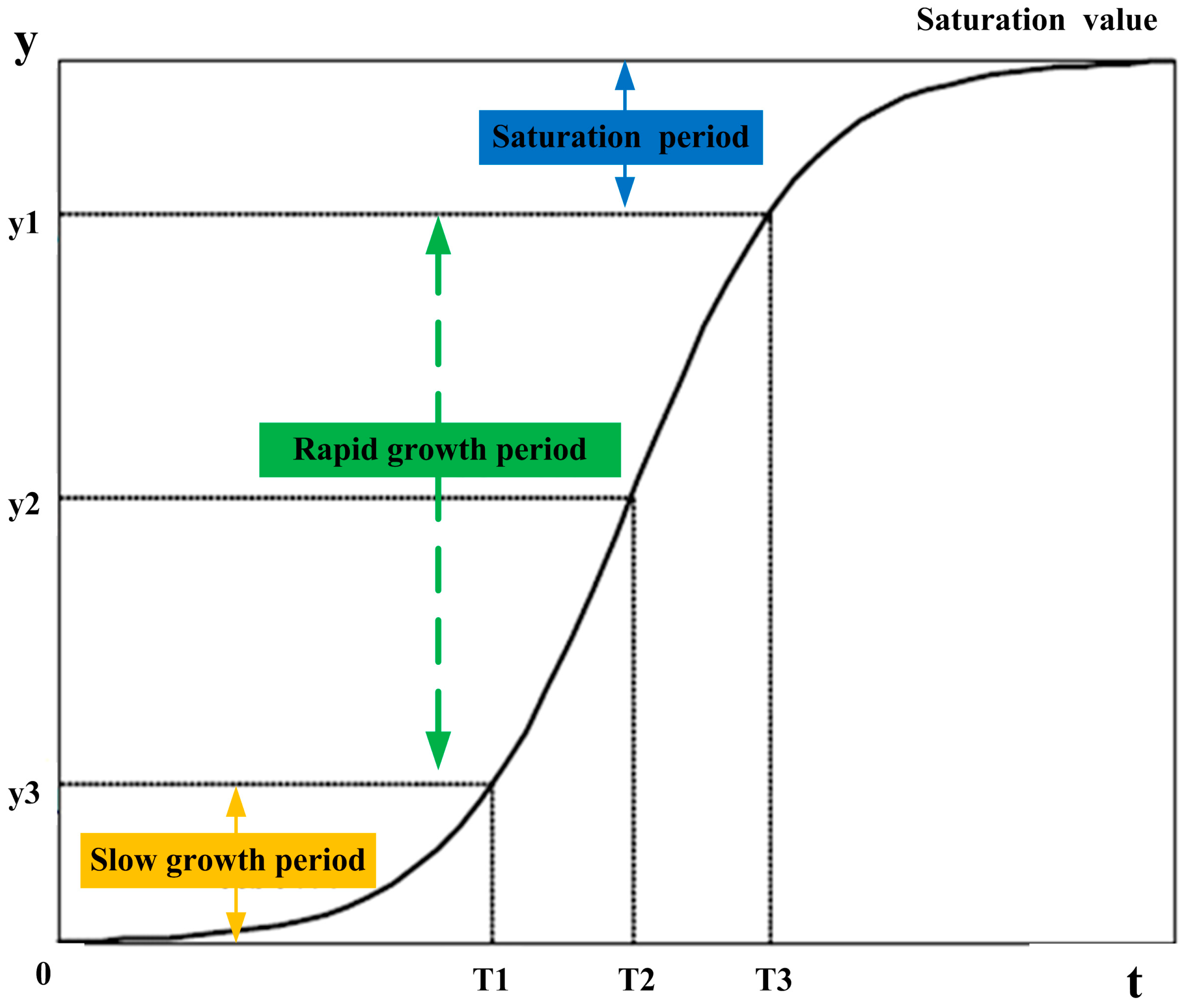
2.1. Basic Principle of the Logistic Curve Model

The logistic curve model is a kind of growth curve model that was first used to predict population growth and then widely used in the fields of growth, development and reproduction of flora and fauna, socio-economic issues, and so on [22,23,24]. The characteristics of the logistic curve model are as follows: in the beginning, the object grows slowly; when it reaches a certain period, the object grows rapidly; and after the object reaches a limit value, its growth rate slows again. These characteristics correspond to those of power loads [2,3,4,5,13]. Therefore, the logistic curve model can be used for saturated power load analysis.

The mathematical expression of the logistic curve model is:

$$y=\frac{k}{1+a{e}^{-bt}}$$

(1)

where k, a, b are constants, and k > 0, a > 0, b > 0.

The logistic curve shape is shown in Figure 1.

Figure 1. Logistic curve shape.

Figure 1. Logistic curve shape.

According to Equation (1), the first-order derivative value of the logistic curve equation at any point is always positive. At point (T₂, y₂), the second-order derivative value equals 0, and at points (T₁, y₁) and (T₃, y₃), the third-order derivative value equals 0. For the logistic curve, as shown in Figure 1, when t is in the interval [0, T₁], y is at the initial slow growth stage; when t is in the interval [T₁, T₃], y is at the rapid growth stage; when t is in the interval [T₃, +∞], y is at the saturated growth stage; and when t is in the interval [T₂, T₃], y displays a slowing growth rate compared to that in interval [T₁, T₂], and gradually becomes saturated.

When the logistic curve model is used for saturated power load forecasting, the input variable is the historical power load data.

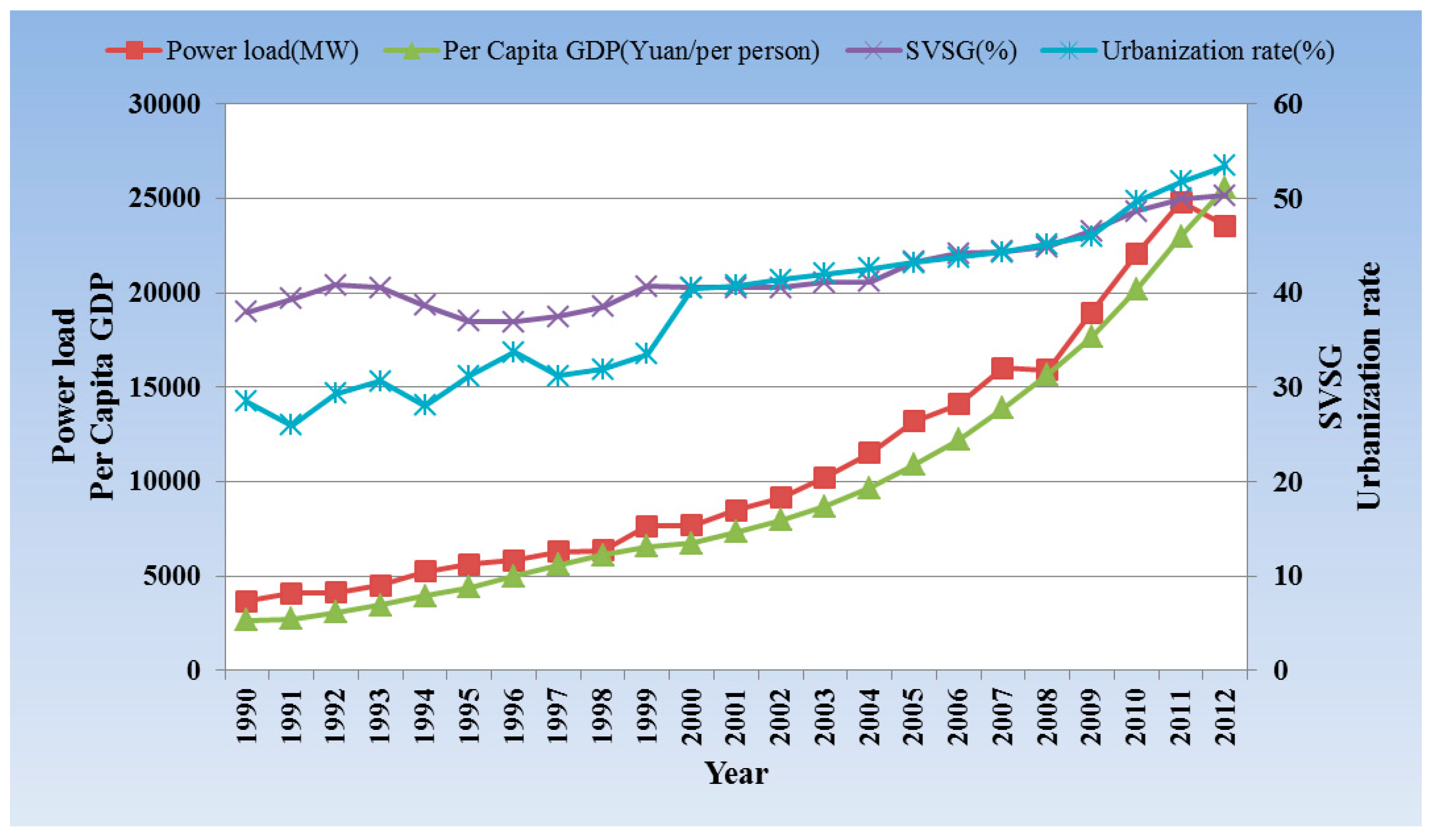
2.2. Basic Principle of the Multi-Dimensional Saturated Power Load Forecasting Model (MSPLF)

In reality, most complex issues are often influenced by many factors. The saturated scale and time of a province’s or city’s power load will also be influenced by many factors, such as regional economic development conditions, social development, population size, energy structure, technological development level, and so on.

Given the above, the MSPLF model uses the factors influencing urban power load as the independent variables and takes power load as the dependent variable, to establish the appropriate mathematical model. Specifically, the MSPLF model can be expressed as:

$$y=f(x_1,x_2,\cdots ,x_n)$$

(2)

where $x_i$ is the influencing factor and $y$ is the power load. The MSPLF model can be solved by using the ordinary least square (OLS) method.

The MSPLF model is based on econometric principles, and its modeling approach is relatively flexible because one can build linear or non-linear models based on the characteristics of the issue. Meanwhile, the MSPLF model can also be used for sensitivity analysis of the influencing factors by solving the partial derivative of the dependent variable.

2.3. Basic Principle of the CFM

The proposed CFM in this paper combines the logistic curve model and MSPLF model, which both considers the internal development law of load data themselves and the impact of economic and social development factors. For the weights of these two single models in the CFM, a new swarm intelligence optimization algorithm, namely the fruit fly optimization algorithm, is employed for weight optimization and determination.

The fruit fly optimization algorithm (FOA) is a new meta-heuristic algorithm proposed by W.T. Pan in 2011, which has the advantages of being easy to understand due to shorter program code than other optimization algorithms and of quickly reaching the global optimal solution [25]. FOA has been used in many fields, including power load forecasting [26,27]. The fundamental principle and calculation steps of FOA are as follows [25,26,27].

Step 1. Parameters initialization.

The maximum iteration number maxgen, population size sizepop, initial fruit fly swarm location (X_axis，Y_axis), and random flight distance range FR are the main parameters of the FOA. When employing the FOA, the initial values of these parameters need to be set first.

Step 2. Population initialization.

Give the random flight direction and the distance for food finding of an individual fruit fly by using osphresis, and then (X_i, Y_i) can be obtained.

$$X_i=X\_axis+\mathrm{Random\; Value}$$

(3)

$$Y_i=Y\_axis+\mathrm{Random\; Value}$$

(4)

Step 3. Population evaluation.

Firstly, the distance of the food location to the origin (Dist) needs to be calculated. Secondly, the smell concentration judgment value (S) needs to be calculated, and the value of S is the reciprocal of the distance of the food location to the origin (Dist), which is reasonable because the longer the distance, the smaller the smell concentration.

$$Dis{t}_i={({X_i}^2+{Y_i}^2)}^{1/2}$$

(5)

$$S_i=1/Dis{t}_i$$

(6)

Then, calculate the smell concentration (Smell_i) of the individual fruit fly location by substituting the smell concentration judgment value (S_i) into the smell concentration judgment function (also called fitness function). Finally, determine the individual fruit fly with the maximal smell concentration (the maximal value of Smell_i) among the fruit fly swarm.

$$Smel{l}_i=\mathrm{Function} \left(S_i\right)$$

(7)

$$[bestSmell bestIndex]=\max \left(Smel{l}_i\right)$$

(8)

Step 4. Selection operation.

Keep the maximal smell concentration value and x, y coordinate. Then, the fruit fly swarm flies towards that location with the maximal smell concentration value by using vision. Enter iterative optimizations to repeat the implementation of Steps 2 and 3. When the iterative number reaches the maximal iterative number or the smell concentration is no longer superior to the previous iterative one, the circulation stops. Then, the final parameter values can be obtained.

$$Smellbest=bestSmell$$

(9)

$$X\_axis=X \left(bestIndex\right)$$

(10)

$$Y\_axis=Y \left(bestIndex\right)$$

(11)

The process of employing the proposed CFM to analyze the saturated power load is shown in Figure 2, and the specific steps are as follows.

Step 1: Using the logistic curve model and MSPLF model to fit the original data.

The sample data is divided into training data and testing data. Using the logistic curve model and MSPLF model to fit the training data, the logistic curve equation and MSPLF equation can be obtained. Then, the fitting values of these two models in the training period can be obtained, which will be used as input data in the CFM for determining the weights.

Step 2: Using the FOA to determine the weights of the logistic curve model and MSPLF model in the proposed CFM.

(1)

Initialization parameters.

The maximum iteration number maxgen, the population size sizepop, the initial fruit fly swarm location (X_axis, Y_axis), and the random flight distance range FR are determined first.

(2)

Evolution starts.

Set i = 1, gen = 0, and give the random flight direction rand() and the flight distance for food finding for an individual fruit fly i. In the hybrid forecasting model, two variables (X(i,:), Y(i,:)) are employed to represent the flight distance for food finding for an individual fruit fly i, and set X(i,:) = X_axis + 20*rand() − 10, Y(i,:) = Y_axis + 20*rand() − 10, respectively.

(3)

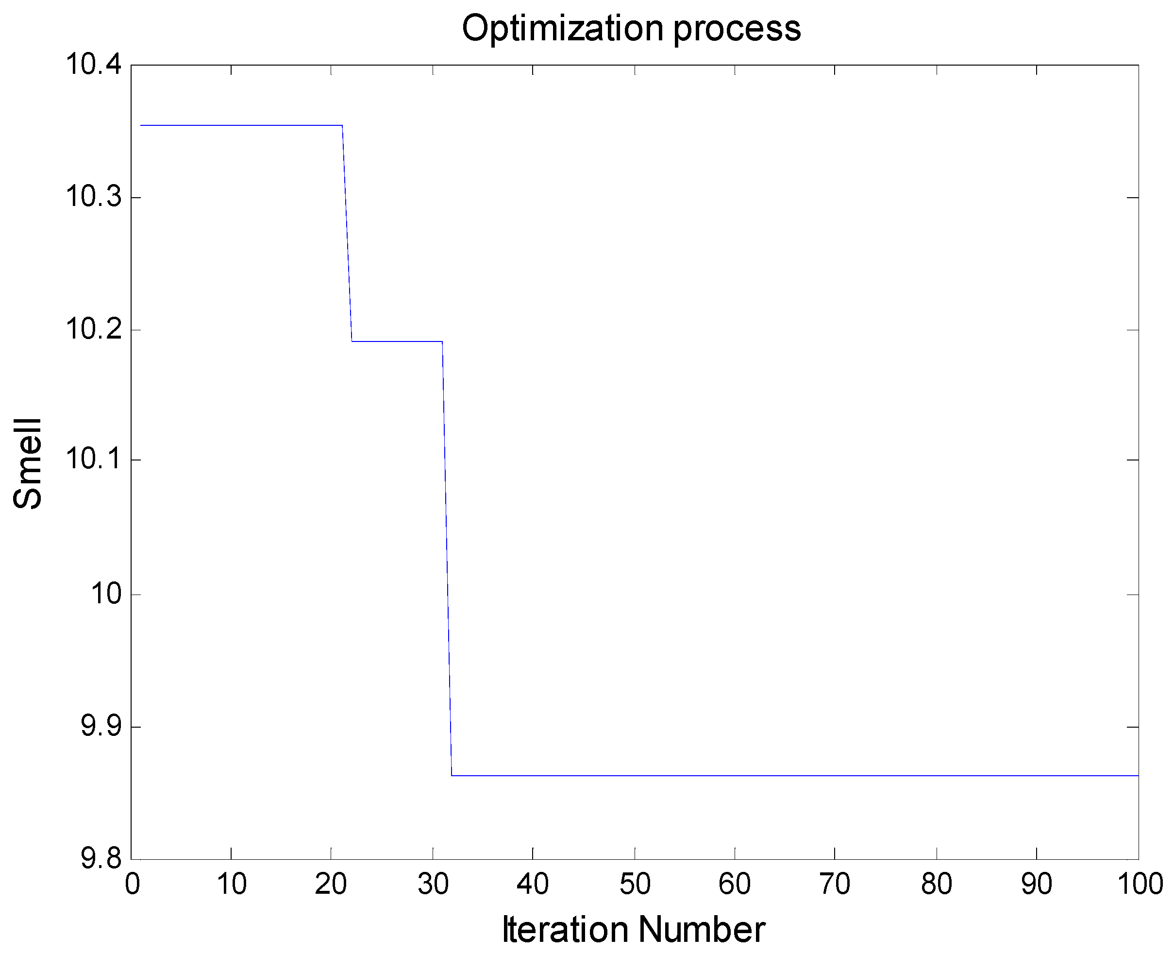
Preliminary calculations.

Update the coordinate (X(i,:), Y(i,:)) of the i-th fly fruit, calculate the distance Dist_i of the fruit fly i to the origin, and then calculate the smell concentration judgment value S_i. In the hybrid forecasting model, (D(i,1), D(i,2)) is employed to represent Dist_i, and set D(i,1) = (X(i,1)² + Y(i,1)²)^0.5, D(i,2) = (X(i,2)² + Y(i,2)²)^0.5, respectively. Similarly, (S(i,1), S(i,2)) is used to represent S_i in the hybrid forecasting model, and set S(i,1) = 1/D(i,1), S(i,2) = 1/D(i,2), respectively. Then, input S_i into the hybrid forecasting model for power load forecasting. In the hybrid forecasting model, the parameters [w₁, w₂] are represented by [S(i,1), S(i,2)], and we set w₁ = S(i,1) and w₂ = S(i,2), respectively. According to the power load forecasting result, the smell concentration Smell_i (also called the fitness function value) can be calculated. The Smell_i is employed by Equation (12), which measures the deviations between the forecasting values and actual values.

$$Smel{l}_i=\frac{1}{n}\sqrt{{\displaystyle \sum _{i=1}^n{\left(w_1{F}_i^L+w_2{F}_i^D-A_i\right)}^2}}$$

(12)

where n is the number of forecasting periods; $A_i$ is the actual value at period i; $F_i^L$ and $F_i^D$ denotes the forecasting value of the logistic curve model and MSPLF model at period i, respectively; and $w_1$ and $w_2$ are the weight of the logistic curve model and MSPLF model in the hybrid model, respectively.

(4)

Population iteration.

Set i = i + 1 and repeat (3). When i equals the population size, find and keep the minimum smell concentration value among the fruit fly swarm, and update (X_axis, Y_axis) and Smellbest.

(5)

Offspring generation.

Generate the offspring generation, and input the offspring into the hybrid forecasting model and calculate the smell concentration value again. Set gen = gen + 1.

(6)

Circulation stops.

When gen reaches the max iterative number, the stop criterion is satisfied and the optimal parameters $w_1$ and $w_2$ of CFM are obtained. Otherwise, go back to (3).

Step 3: Using the proposed CFM to forecast the power load.

After obtaining the power load fitting values from the logistic curve model and MSPLF model and the mathematical weights, the load forecasting value can be calculated by using the proposed CFM according to Equation (13).

$$F_i^H=w_1{F}_i^L+w_2{F}_i^D$$

(13)

where $F_i^H$, $F_i^L$ and $F_i^D$ are the forecasting values of the proposed CFM, the logistic curve model and the MSPLF model at time i, respectively.

Step 4: Saturated power load analysis.

According to the judging criteria for power load saturation, the saturated time and saturated load value of a province’s or city’s power load can be obtained.

Figure 2. Flow chart of the proposed CFM for saturated power load analysis.

Figure 2. Flow chart of the proposed CFM for saturated power load analysis.

3. Forecasting Performance Test of Proposed CFM

To test the forecasting performance of the proposed CFM, the single logistic curve model and the MSPLF model are selected as the comparison models. Using Hubei Province as the empirical example, the forecasting errors of these three models will be discussed. For the logistic curve model, the power load is the only input factor. For the MSPLF model, several factors which have relatively close relationships with power load are required as the input factors. Commonly, there are relevant relationships between urban power load and economic social factors, such as regional GDP, population, industrial structure, urbanization level and so on [2,3,4,5,6,10,13]. Therefore, GDP per capita, share of value-added from secondary industry in GDP (SVSG) and urbanization rate were selected as the input variables of MSPLF model.

Therefore, when employing the CFM to an analysis of urban saturated power load, the power load, GDP per capita, SVSG and urbanization rate are needed. The sample data are taken from 1900 to 2012. Of this range, the data from 1900 to 2005 are selected as a training sample, and the data from 2006 to 2012 are the testing sample. The development trends in annual maximum power load, GDP per capita, SVSG and urbanization rate of Hubei Province from 1990 to 2012 are shown in Figure 3.

Figure 3. Development trend of annual maximum power load, per capita GDP, SVSG and urbanization rate of Hubei Province from 1990 to 2012.

Figure 3. Development trend of annual maximum power load, per capita GDP, SVSG and urbanization rate of Hubei Province from 1990 to 2012.

3.1. Forecasting Result of the Logistic Curve Model

Using the annual maximum power load of Hubei Province from 1990 to 2005 as the fitting sample data, the fitting result of the logistic curve in term of annual maximum power load using MATLAB software v2014a is shown in Figure 4. Meanwhile, the logistic curve equation in term of annual maximum power load can be obtained, i.e.:

$$y^L=\frac{7700}{1+19.47e^{-0.0948t}}$$

(14)

The fitting performance index R² of the logistic curve equals 0.985, which shows the fitting result is quite good.

Figure 4. Fitting result of the logistic curve model in terms of annual maximum power load.

Figure 4. Fitting result of the logistic curve model in terms of annual maximum power load.

Then, according to Equation (14), the annual maximum power load of Hubei Province from 2006 to 2012 can be forecasted by employing the logistic curve model, and the result is shown in Table 1.

Table 1. Power load forecasting result of the logistic curve model.

Year	2006	2007	2008	2009	2010	2011	2012
Annual maximum power load (104 kW)	1461	1576	1698	1827	1962	2104	2252

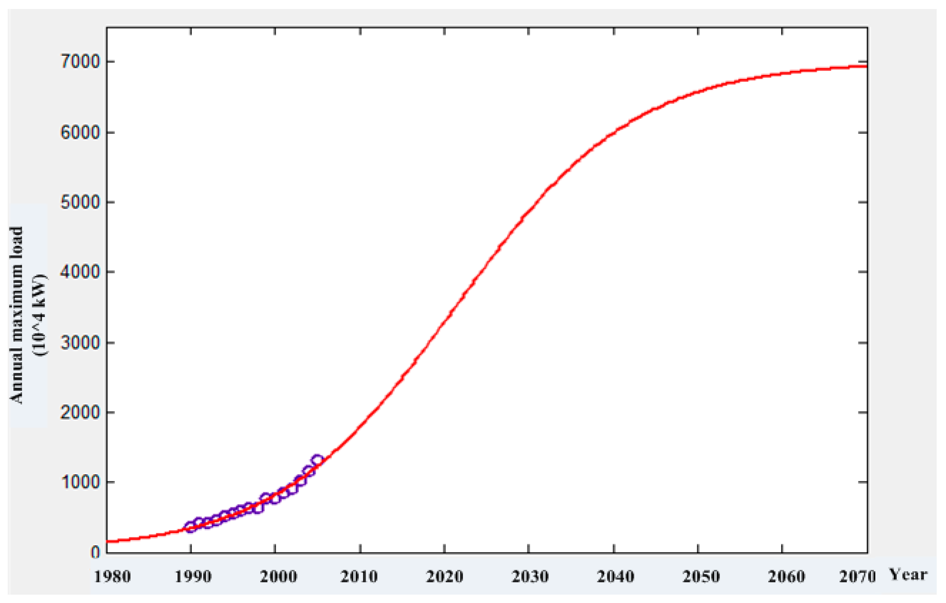
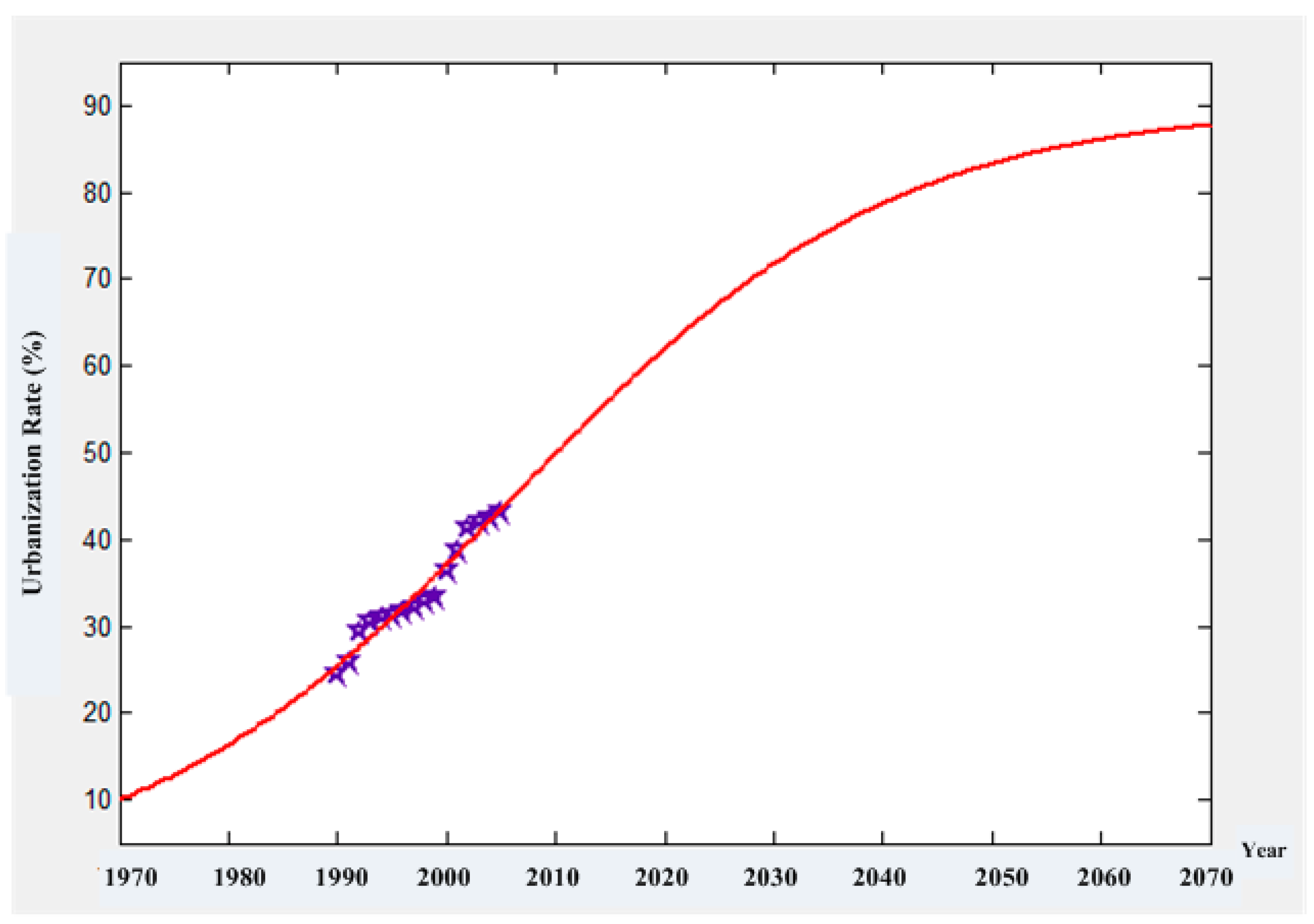
Table 1. Power load forecasting result of the logistic curve model.

Year	2006	2007	2008	2009	2010	2011	2012
Annual maximum power load (104 kW)	1461	1576	1698	1827	1962	2104	2252

3.2. Forecasting Result of the MSPLF Model

Three factors, namely GDP per capita, SVSG and urbanization rate are selected as the input variables of the MSPLF model. According to Equation (2), the fitting equation of the MSPLF model for power load forecasting can be obtained by employing the OLS method, as shown in Equation (15).

$$y^M=0.1108PGDP-9.5974SVSG+2.5928UR+338.7261$$

(15)

where PGDP represents GDP per capita; SVSG represents the share of value-added of secondary industry in GDP; and UR represents the urbanization rate. The fitting performance index R² of MSPLF equals 0.9846, which indicates that the fitting performance is quite good.

Then, according to Equation (15), the annual maximum power load of Hubei Province from 2006 to 2012 can be forecasted by employing the MSPLF model, and the result is listed in Table 2.

Table 2. Power load forecasting result of the MSPLF model.

Year	2006	2007	2008	2009	2010	2011	2012
Annual maximum power load (104 kW)	1383	1567	1763	1968	2235	2541	2830

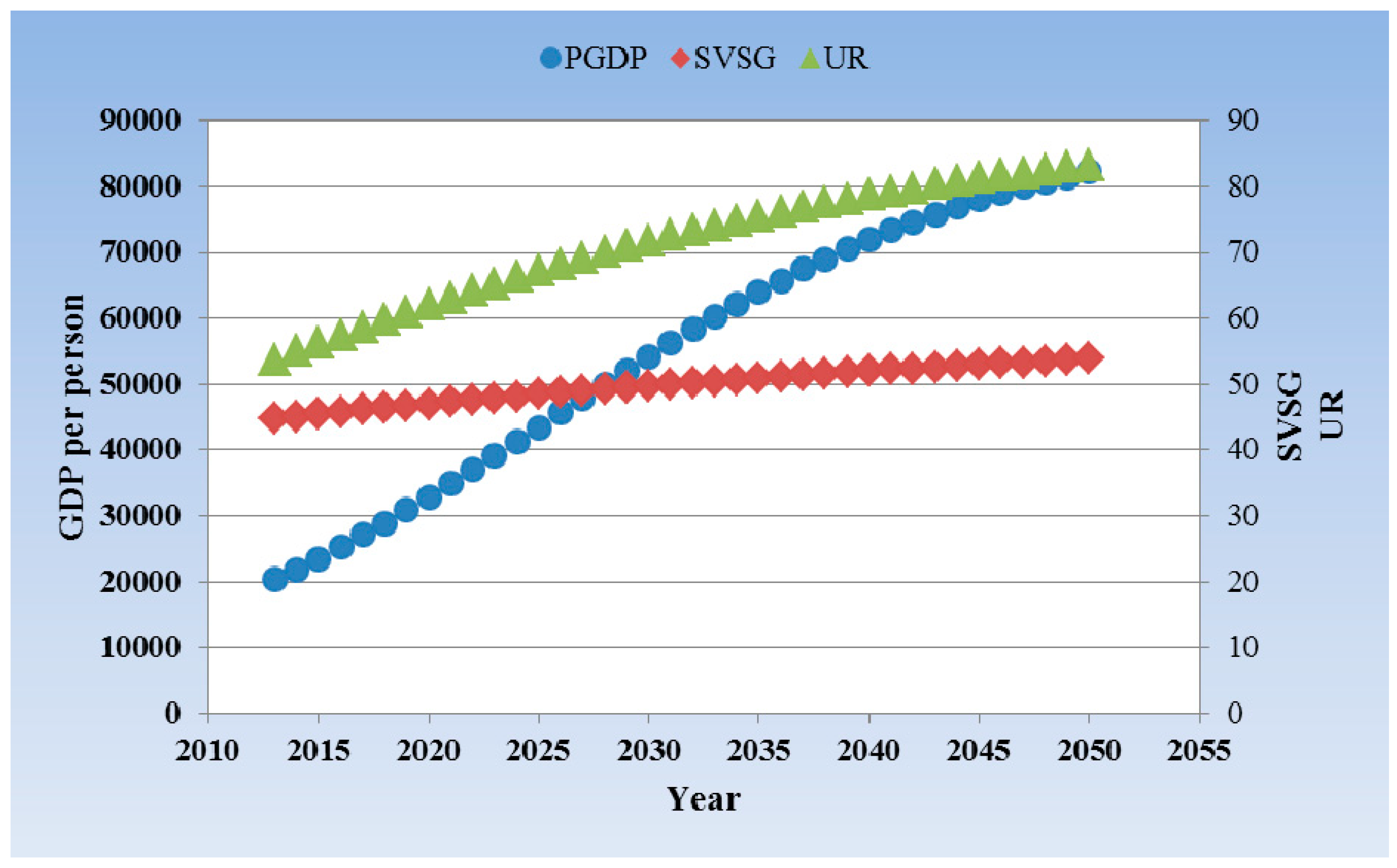
Table 2. Power load forecasting result of the MSPLF model.

Year	2006	2007	2008	2009	2010	2011	2012
Annual maximum power load (104 kW)	1383	1567	1763	1968	2235	2541	2830

3.3. Forecasting Result of the CFM

When using the CFM to forecast power load, the weights of the logistic curve model and MSPLF model, namely w₁ and w₂ in Equation (13), first need to be determined. As mentioned above, the FOA is employed to iteratively determine the optimal value of w₁ and w₂. The initial parameters of the FOA are set as follows: maxgen = 100, sizepop = 20, (X_axis, Y_axis) $\subset$ [−50, 50], FR $\subset$ [−10, 10], X_axis = rands(1, 2), Y_axis = rands(1, 2). Figure 5 shows the iterative Smell trend for the CFM searching for optimal parameters. After 100 evolution iterations, convergence can be seen in generation 32. Finally, the optimal values of parameters w₁ and w₂ are 0.557 and 0.443, respectively.

Figure 5. Iterative Smell trend for the CFM searching for optimal parameters.

Figure 5. Iterative Smell trend for the CFM searching for optimal parameters.

Then, based on the forecasting results of the logistic curve model and MSPLF model from 2006 to 2012, the annual maximum power load of Hubei Province from 2006 to 2012 can be forecasted by employing the proposed CFM based on Equation (13), and the result is listed in Table 3.

Table 3. Power load forecasting result of the proposed CFM.

Year	2006	2007	2008	2009	2010	2011	2012
Annual maximum power load (104 kW)	1426	1572	1727	1890	2083	2298	2508

Table 3. Power load forecasting result of the proposed CFM.

Year	2006	2007	2008	2009	2010	2011	2012
Annual maximum power load (104 kW)	1426	1572	1727	1890	2083	2298	2508

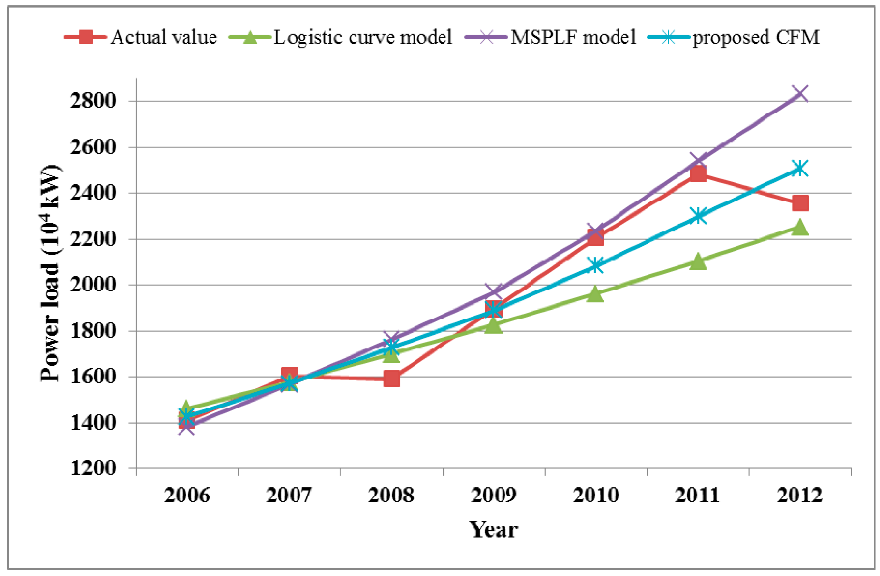
3.4. Comparison of Forecasting Results

The forecasting results of the logistic curve model, MSPLF model and proposed CFM model and the actual power load are shown in Figure 6. From Figure 6, it can be seen that the forecasting values of the logistic curve model in 2007, 2008 and 2012 have the smallest deviations from the actual power load; the forecasting values of the MSPLF model in 2010 and 2011 have the smallest deviations from the actual power load; and the forecasting values of the proposed CFM model in 2006 and 2009 have the smallest deviations from the actual power load. Although the proposed CFM model does not obtain the largest number of the smallest deviation forecasting years, the forecasting results in other non-dominated years show smaller deviations from the actual power load.

Figure 6. Comparisons of forecasting values of different models and actual power load.

Figure 6. Comparisons of forecasting values of different models and actual power load.

Further, in order to accurately test the forecasting performances of different forecasting models, the forecasting errors of different forecasting models need to be compared. The mean absolute percentage error (MAPE), mean square error (MSE) and mean relative error (MRE) were selected for the forecasting error analysis indicators, which can be calculated as follows:

$$MAPE=\frac{1}{n}{\displaystyle \sum _{i=1}^n\left|\frac{A_i-F_i}{A_i}\right|}\times 100\%$$

(16)

$$MSE=\frac{1}{n}{\displaystyle \sum _{i=1}^n{(A_i-F_i)}^2}$$

(17)

$$MRE=\frac{1}{n}{\displaystyle \sum _{i=1}^n\frac{A_i-F_i}{A_i}}\times 100\%$$

(18)

where $A_i$ is the actual value of annual maximum power load at the i-th year, and $F_i$ is the forecasting value of annual maximum power load at the i-th year.

The forecasting error comparisons of the logistic curve model, MSPLF model and proposed CFM are shown in Figure 7. It can be seen that the MAPE value of the proposed CFM is 4.50%, which is much lower than that of the logistic curve model and MSPLF model (which are 6.64% and 6.09%, respectively). The MSE value of the proposed CFM is 13,148, which is dramatically lower than that of the logistic curve model and MSPLF model (which are 33,341 and 37,835, respectively). The MRE value of the proposed CFM is 0.11%, which is much lower than that of the logistic curve model and MSPLF model (which are −3.69% and 4.87%, respectively).

Figure 7. Forecasting error comparisons of different models.

Figure 7. Forecasting error comparisons of different models.

Conclusively, the proposed CFM largely narrows the deviations between the forecasting values and actual values, and outperforms the logistic curve model and MSPLF model in annual maximum power load forecasting. Therefore, the proposed CFM in this paper is very suitable for saturated power load analysis.

4. Empirical Analysis of Saturated Power Load

When using the proposed CFM to analyze the saturated power load, firstly, the power load of Hubei Province in future years (2013–2050 in this paper) should be forecasted by using the logistic curve model and MSPLF model, and then the power load forecasting value of the proposed CFM from 2013 to 2050 should be calculated according to Equation (13); secondly, according to the judgment criteria for saturated power load and the power load forecasting result, the saturated time and scale for Hubei Province’s power load can be obtained.

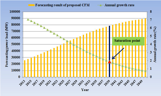
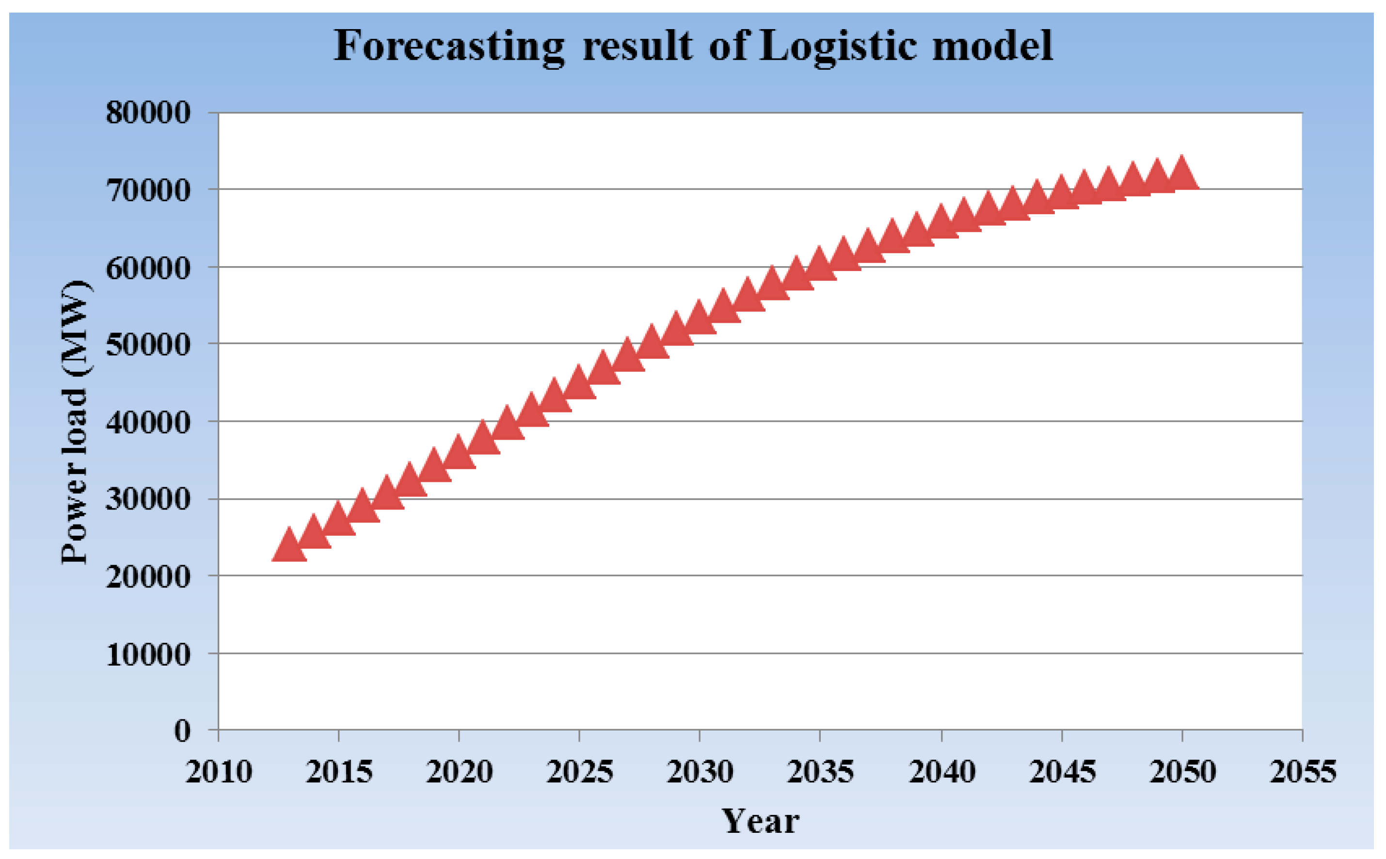
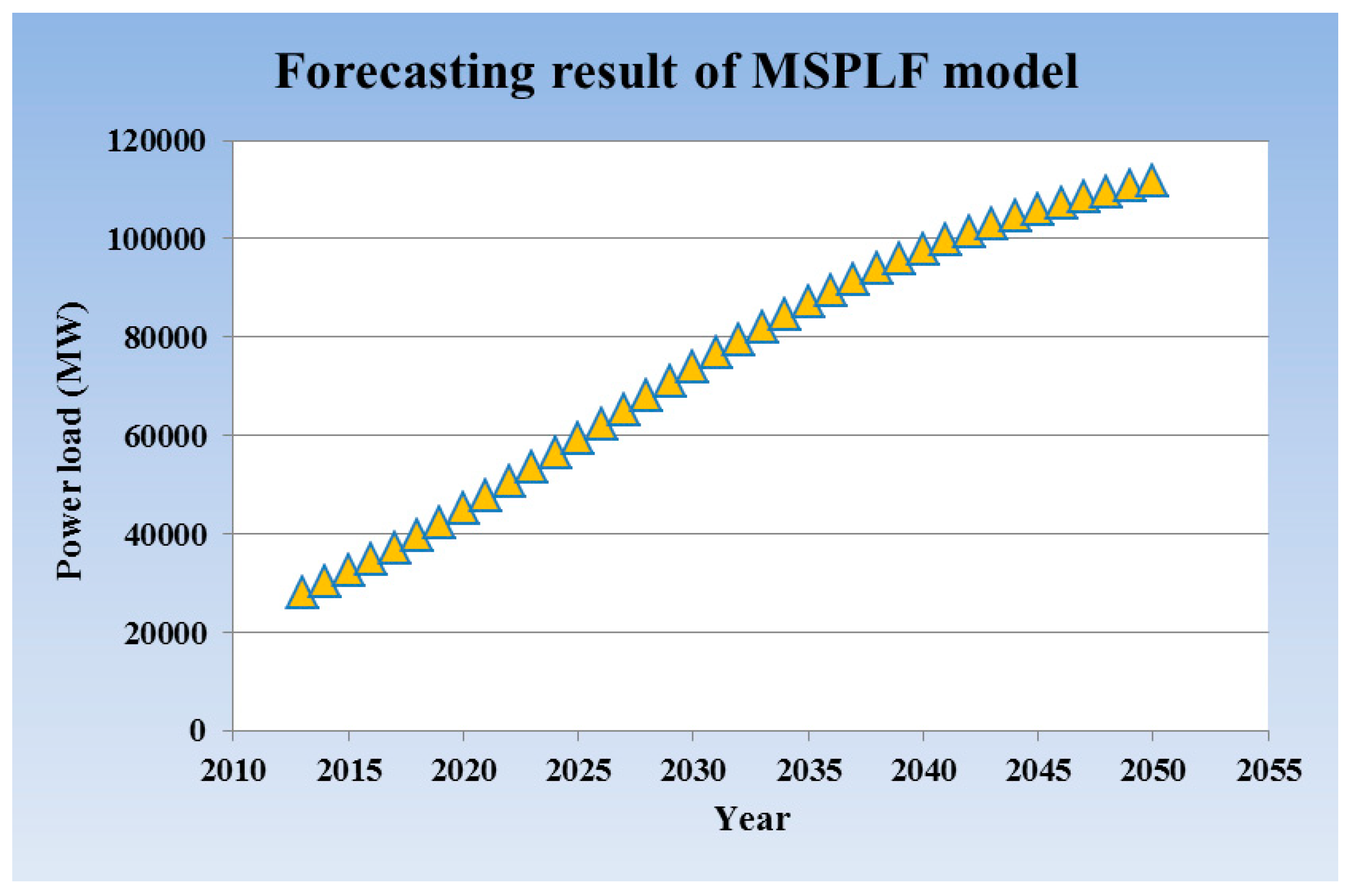
4.1. Forecasting Result for Power Load from 2013 to 2050

According to Equation (14), the forecasting result for the annual maximum power load of Hubei Province from 2013 to 2050 according to the logistic curve model can be obtained, as shown in Figure 8. From Figure 8, it can be seen that the forecasted annual maximum power load of Hubei Province according to the logistic curve model will increase to about 70,000 MW in 2050 from 24,062 MW in 2013.

Figure 8. Power load forecasting result from 2013 to 2050 according to the logistic curve model.

Figure 8. Power load forecasting result from 2013 to 2050 according to the logistic curve model.

When using the MSPLF model to forecast the annual maximum power load of Hubei Province, the input variables, namely GDP per capita, SVSG and urbanization rate need first to be forecasted. Urban electric power load saturation is an important way to express the economic social development of a region entering its mature stage. At this time, the relative factors affecting power load, such as regional economy, population and industrial structure, will tend toward a relatively stable size without major fluctuation. Many scientific studies have shown that some factors in the fields of economy, society and population follow the logistic curve development law. Meanwhile, [28,29,30] point out that GDP per capita, SVSG and urbanization rate will gradually reach saturation with economic social development, which can be forecasted using the growth curve model. Therefore, GDP per capita, SVSG and urbanization rate are forecasted using the logistic curve model in this paper. The fitting results of GDP per capita, SVSG and urbanization rate using the logistic curve model are shown in Figure 9, Figure 10 and Figure 11, respectively.

Figure 9. Fitting result of GDP per capita with the logistic curve model.

Figure 9. Fitting result of GDP per capita with the logistic curve model.

Figure 10. Fitting result of SVSG with the logistic curve model.

Figure 10. Fitting result of SVSG with the logistic curve model.

Figure 11. Fitting result of urbanization rate with the logistic curve model.

Figure 11. Fitting result of urbanization rate with the logistic curve model.

The fitting equations for GDP per capita, SVSG and urbanization rate are:

$$y^{PGDP}=\frac{90000}{1+31.86e^{-0.09695t}}$$

(19)

$$y^{SVSG}=\frac{60}{1+0.668e^{-0.02938t}}$$

(20)

$$y^{UR}=\frac{90}{1+2.53e^{-0.0575t}}$$

(21)

From Figure 9, it can be seen that the GDP per capita of Hubei Province before 2010 is at the initial slow growth period; after 2010, it reaches the rapid growth stage. According to the fitting result of the logistic curve model, the GDP per capita of Hubei Province will reach the saturated growth stage at around 2040. From Figure 10, it can be seen that the SVSG of Hubei Province has been at the rapid growth stage since the sample years, but it shows a slowing growth rate in the past few years. According to the fitting result of the logistic curve model, the SVSG of Hubei Province will reach the saturated growth stage at around 2035. From Figure 11, the urbanization rate of Hubei Province is at the rapid growth stage, but the growth rate is currently decreasing, and the urbanization rate of Hubei Province will reach the saturated growth stage at around 2038. Therefore, based on the forecasting saturation time of GDP per capita, SVSG and urbanization rate, we can roughly judge that the power load of Hubei Province will reach saturation at around 2040.

The forecasting values of GDP per capita, SVSG and urbanization rate of Hubei Province from 2013 to 2050 can be obtained, as shown in Figure 12.

Figure 12. Forecasting values of GDP per capita, SVSG and urbanization rate of Hubei Province from 2013 to 2050.

Figure 12. Forecasting values of GDP per capita, SVSG and urbanization rate of Hubei Province from 2013 to 2050.

According to Equation (15), the annual maximum power load of Hubei Province from 2013 to 2050 by using the MSPLF model can be calculated, and the result is shown in Figure 13. From Figure 13, we can see that the forecasted annual maximum power load of Hubei Province according to the MSPLF model will increase to about 110,000 MW in 2050 from 28,078 MW in 2013, which is much higher than that of the logistic curve model.

Figure 13. Forecasting result of Hubei Province’s power load from 2013 to 2050 according to the MSPLF model.

Figure 13. Forecasting result of Hubei Province’s power load from 2013 to 2050 according to the MSPLF model.

Based on the forecasting results of the logistic curve model and MSPLF model from 2013 to 2050, the annual maximum power load of Hubei Province from 2013 to 2050 can be forecasted by employing the proposed CFM according to Equation (13), and the result is shown in Figure 14. From Figure 14, it can be seen that the forecasted annual maximum power load of Hubei Province according to the proposed CFM model will increase to nearly 90,000 MW in 2050 from 25,841 MW in 2013, which is much lower than that of the MSPLF model, and higher than that of the logistic curve model. Meanwhile, the annual growth rate of the maximum power load of Hubei Province will decline from about 7% in 2013 to less than 2% after 2039.

Figure 14. Power load forecasting result from 2013 to 2050 by using the proposed CFM.

Figure 14. Power load forecasting result from 2013 to 2050 by using the proposed CFM.

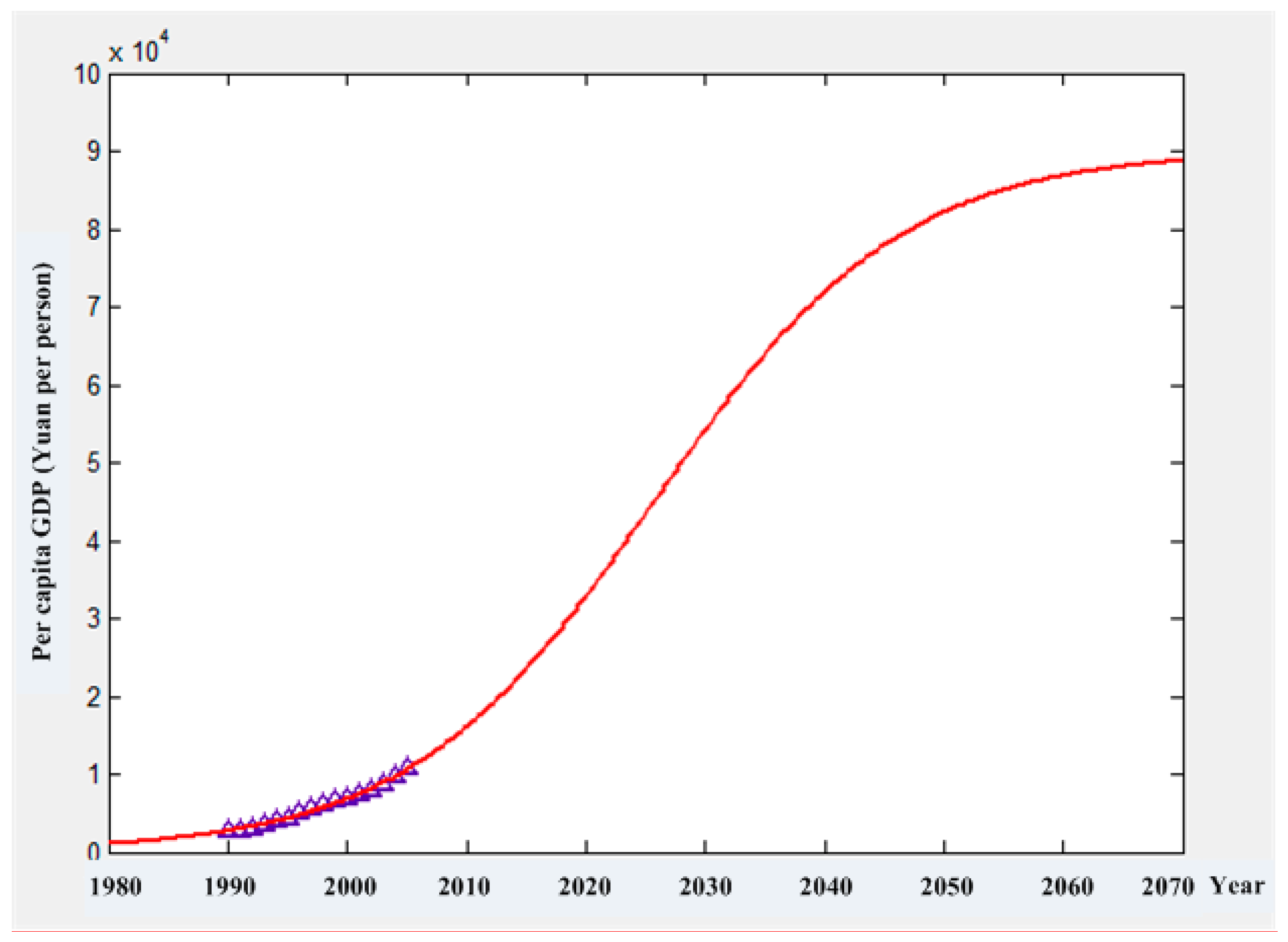
4.2. Saturation Analysis

According to Reference [13], when the annual growth rate of a region’s power load is less than 2%, it can be concluded that the electricity demand in this region has reached saturation. In Figure 14, the annual growth rate of Hubei Province’s power load has been on a downward trend, and it will fall to 1.898% in 2039, which is the first year that the annual growth rate is less than 2%. Therefore, we can safely conclude that the electricity demand in Hubei Province will reach saturation in 2039. At this time, the annual maximum power load, GDP per capita, SVSG and urbanization rate will reach 78,629.25 MW, 70,561.03 RMB per capita, 51.8% and 78.18%, respectively.

5. Conclusions

Power load forecasting is the foundation of urban power grid planning, and saturated power load is a key indicator for determining the ultimate power grid scale when performing urban power grid planning. Analyzing saturated power load is helpful for determining the ultimate power grid scale and also plays an important role in promoting the healthy and sustainable development of the power grid. In this paper, a novel combined forecasting model is proposed for urban saturated power load analysis based on the logistic curve model and multi-dimensional saturated power load forecasting model, and the mathematical weights of these two single models in the proposed combined forecasting model are optimally determined using the fruit fly optimization algorithm. Using Hubei Province as the empirical example, the analysis results show:

(1)

The forecasting accuracy of the proposed combined forecasting model in this paper is much higher than that of the single logistic curve model and multi-dimensional saturated power load forecasting model, which indicates the proposed CFM is more suitable for saturated power load analysis;

(2)

The annual maximum power load of Hubei Province will reach saturation in 2039, at which time the growth rate of the annual maximum power load will fall to 1.898%, and the annual maximum power load, GDP per capita, SVSG and urbanization rate will reach 78,629.25 MW, 70,561.03 RMB per capita, 51.8% and 78.18%, respectively.

References

- Amin, S.M.; Wollenberg, B.F. Toward a smart grid: Power delivery for the 21st century. IEEE Power Energy Mag. 2005, 3, 34–41. [Google Scholar] [CrossRef]
- Cui, K.; Li, J.; Liu, H.; Yang, W.; Yuan, Z. City’s Power Planning Methods at the Stage of Load Saturation and Its Application in Jinan Power Grid. Power Syst. Technol. 2007, 31, 131–134. [Google Scholar]
- Cui, K.; Li, J.; Zhao, B.; Liu, H. Research on City Saturated Load and its Forecast Methods. Electr. Power Technol. Econ. 2008, 20, 34–38. [Google Scholar]
- Jiang, X.; Li, X. City future saturated load forecasting based model of saturated load density. J. Fuzhou Univ. (Nat. Sci. Edition) 2008, 36, 532–536. [Google Scholar]
- Xiao, X.; Zhou, Y.; Zhang, N. Survey of saturated load analysis technology for urban power system and its application. Electr. Power Autom. Equip. 2014, 34, 146–152. [Google Scholar]
- Zhang, J.; Liu, J.; Chen, Y. Saturated Load Forecasting Based on Per Capita Electricity Consumption and Per Capita Electricity Load. East China Electr. Power 2014, 42, 661–664. [Google Scholar]
- Jia, Y.; Li, S.; Tan, Y.; Zhao, F.; Hou, F. Improved parametric estimation of logistic model for saturated load forecast. In Proceedings of IEEE PES Asia-Pacific Power and Energy Engineering Conference, Shanghai, China, 26–28 March 2012.
- Bai, C. Application of improved GM (1, 1) power model to middle and long term load forecasting. Water Resour. Power 2011, 29, 177–179. [Google Scholar]
- Zhao, H. Research and application of nonlinear regression correct model in sudden change load forecasting. Math. Pract. Theory 2008, 38, 88–91. [Google Scholar]
- He, H. Forecasting the urban saturated load based on the analysis of land-use change. Master’s Thesis, North China Electric Power University, Beijing, China, 2012. [Google Scholar]
- Wang, W.; Fang, T. The application of per-person electricity consumption method in saturation load forecasting. Power Demand Side Manag. 2012, 14, 21–23. [Google Scholar]
- He, Y.; Wu, L.; Dai, A.; Yang, W.; Wang, Y. Combined saturation load forecast model based on system dynamics and econometrics. Power Demand Side Manag. 2010, 12, 21–25. [Google Scholar]
- Liu, J. The Research of Saturation Load Analysis Techniques and its Application. Master’s Thesis, Shanghai Jiaotong University, Shanghai, China, 2013. [Google Scholar]
- Bates, J.M.; Granger, C.W.J. Combination of forecasts. Oper. Res. Q. 1969, 20, 451–468. [Google Scholar] [CrossRef]
- Huang, S.J.; Shih, K.R. Short-term load forecasting via ARMA model identification including non-Gaussian process considerations. IEEE Trans. Power Syst. 2003, 18, 673–679. [Google Scholar] [CrossRef]
- Pai, P.F.; Hong, W.C. Forecasting regional electricity load based on recurrent support vector machines with genetic algorithms. Electr. Power Syst. Res. 2005, 74, 417–425. [Google Scholar] [CrossRef]
- Kim, K.H.; Youn, H.S.; Kang, Y.C. Short-term load forecasting for special days in anomalous load conditions using neural networks and fuzzy inference method. IEEE Trans. Power Syst. 2000, 15, 559–565. [Google Scholar]
- Hanmandlu, M.; Chauhan, B.K. Load forecasting using hybrid models. IEEE Trans. Power Syst. 2011, 26, 20–29. [Google Scholar] [CrossRef]
- Ko, C.N.; Lee, C.M. Short-term load forecasting using SVR (support vector regression)-based radial basis function neural network with dual extended Kalman filter. Energy 2013, 49, 413–422. [Google Scholar] [CrossRef]
- Selakov, A.; Cvijetinović, D.; Milović, L.; Mellon, S.; Bekut, D. Hybrid PSO–SVM method for short-term load forecasting during periods with significant temperature variations in city of Burbank. Appl. Soft Comput. 2014, 16, 80–88. [Google Scholar] [CrossRef]
- Chen, Y. Validity Theory of Combined Forecasting Model and Its Application; Beijing Science Press: Beijing, China, 2008. [Google Scholar]
- Lemeshow, S.; Hosmer, D.W. A review of goodness of fit statistics for use in the development of logistic regression models. Am. J. Epidemiol. 1982, 115, 92–106. [Google Scholar] [PubMed]
- Mood, C. Logistic regression: Why we cannot do what we think we can do, and what we can do about it. Eur. Sociol. Rev. 2010, 26, 67–82. [Google Scholar] [CrossRef]
- Pradhan, B.; Lee, S. Delineation of landslide hazard areas on Penang Island, Malaysia, by using frequency ratio, logistic regression, and artificial neural network models. Environ. Earth Sci. 2010, 60, 1037–1054. [Google Scholar] [CrossRef]
- Pan, W.T. A new fruit fly optimization algorithm: Taking the financial distress model as an example. Knowl.-Based Syst. 2012, 26, 69–74. [Google Scholar] [CrossRef]
- Li, H.; Guo, S.; Li, C.; Sun, J. A hybrid annual power load forecasting model based on generalized regression neural network with fruit fly optimization algorithm. Knowl.-Based Syst. 2013, 37, 378–387. [Google Scholar] [CrossRef]
- Li, H.; Guo, S.; Zhao, H.; Su, C.; Wang, B. Annual electric load forecasting by a least squares support vector machine with a fruit fly optimization algorithm. Energies 2012, 5, 4430–4445. [Google Scholar] [CrossRef]
- Wang, B.; Ji, F.; Zhou, M. Study on evolutional process of coal industry chain system based on Logistic model. Math. Pract. Theory 2013, 43, 10–17. [Google Scholar]
- Shi, Z.; Huang, H.; Liu, J. Fluctuation analysis of China’s business cycle and forecasting of main Macroeconomic indicators. J. Quant. Tech. Econ. 2007, 24, 14–22. [Google Scholar]
- Huang, H.; Ma, F.; Ma, Y. Logistic curve model for regional economy medium-term and long-term forecast. J. Wuhan Univ. Technol. (Inf. Manag. Eng.) 2011, 33, 94–97. [Google Scholar]
© 2015 by the authors; licensee MDPI, Basel, Switzerland. This article is an open access article distributed under the terms and conditions of the Creative Commons Attribution license (http://creativecommons.org/licenses/by/4.0/).
Share and Cite
Zhao, H.; Guo, S.; Xue, W. Urban Saturated Power Load Analysis Based on a Novel Combined Forecasting Model. Information 2015, 6, 69-88. https://doi.org/10.3390/info6010069
Zhao H, Guo S, Xue W. Urban Saturated Power Load Analysis Based on a Novel Combined Forecasting Model. Information. 2015; 6(1):69-88. https://doi.org/10.3390/info6010069
Chicago/Turabian StyleZhao, Huiru, Sen Guo, and Wanlei Xue. 2015. "Urban Saturated Power Load Analysis Based on a Novel Combined Forecasting Model" Information 6, no. 1: 69-88. https://doi.org/10.3390/info6010069