Article

An Enhanced Quantum-Behaved Particle Swarm Optimization Based on a Novel Computing Way of Local Attractor

College of Electronic and Information Engineering, Southwest University, Chongqing 400715, China
*
Author to whom correspondence should be addressed.
Information 2015, 6(4), 633-649; https://doi.org/10.3390/info6040633
Submission received: 14 July 2015 / Revised: 4 October 2015 / Accepted: 6 October 2015 / Published: 13 October 2015
(This article belongs to the Section Information Theory and Methodology)

Abstract

:
Quantum-behaved particle swarm optimization (QPSO), a global optimization method, is a combination of particle swarm optimization (PSO) and quantum mechanics. It has a great performance in the aspects of search ability, convergence speed, solution accuracy and solving robustness. However, the traditional QPSO still cannot guarantee the finding of global optimum with probability 1 when the number of iterations is limited. A novel way of computing the local attractor for QPSO is proposed to improve QPSO’s performance in global searching, and this novel QPSO is denoted as EQPSO during which we can guarantee the particles are diversiform at the early stage of iterations, and have a good performance in local searching ability at the later stage of iteration. We also discuss this way of computing the local attractor in mathematics. The results of test functions are compared between EQPSO and other optimization techniques (including six different PSO and seven different optimization algorithms), and the results found by the EQPSO are better than other considered methods.

1. Introduction

QPSO (Quantum-behaved Particle Swarm Optimization) is a novel optimization method, which is proposed based on the PSO (Particle Swarm Optimization) algorithm and quantum mechanics. The QPSO algorithm has been greatly improved in the aspects of search ability, convergence speed, solution accuracy and solving robustness, and it can also overcome the shortcoming that the standard PSO (SPSO) cannot guarantee the global convergence [1,2]. For this reason, QPSO has been widely used in bio-medicine, antenna design, combinatorial optimization, signal processing, neural networks and other fields [3,4,5,6,7,8,9,10,11].
Besides QPSO, some other algorithms such as genetic algorithm (GA), evolution strategy with covariance matrix adaptation (CMA-ES) [12], krill herd (KH) [13,14,15], monarch butterfly optimization (MBO) [16], harmony search (HS) [17,18] and artificial plant optimization algorithm (APOA) [19] are also proposed by researchers to solve optimization problems.
The disadvantage of a QPSO algorithm is that it cannot find the global optimum with probability 1 when the number of iterations is limited. The number of total iterations is usually a real number and cannot be set as infinity during the practical application. Therefore, we propose a novel way to compute the local attractor of QPSO to improve the global searching ability of QPSO when the number of iterations is limited. In the rest of this paper, we will firstly introduce the basic theory of SPSO and QPSO, then the proposed way of computing the local attractor is expressed and analyzed. Finally, the enhanced QPSO will be tested by the test functions, and its results are compared with six other PSO algorithms and seven optimization algorithms.

2. QPSO-Based Optimization Algorithm

2.1. Standard Particle Swarm Optimization

PSO is an evolutionary computation algorithm based on swarm intelligence theory. The algorithm comes from the simulation of the bird predation behavior, and its emphases lie in the cooperation and competition between individuals. Because of its rapidity of calculation and ease of implementation, PSO algorithms have been successfully applied in system identification, neural network training, fuzzy system control and other application fields.
In PSO [20], each candidate solution is called a particle and all of the particles are seen to have no quality and volume. Each particle knows its best position, which is called the local optimum. The best position of all the particles is called the global optimum. Suppose a population including M particles moves in a D dimensional space with a certain velocity, then PSO will update the speed and position according to Equations (1) and (2).
V i d ( t ) = V i d ( t 1 ) + c 1 r 1 ( p b e s t i d X i d ( t 1 ) )               + c 2 r 2 ( g b e s t g d X i d ( t 1 ) )
X i d ( t ) = X i d ( t 1 ) + V i d ( t )
where i = 1 ,   2 ,   M , c 1 and c 2 are the learning factors, and generally, c 1 = c 2 = 1 , r 1 and r 2 are the random numbers uniformly distributed between 0 and 1.
To improve the optimization ability, Shi [21,22] put forward a PSO algorithm with an inertial weight ω which can be decreased linearly from 1 to 0.1. Then Equation (1) can be changed to Equation (3).
V i d ( t ) = ω V i d ( t 1 ) + c 1 r 1 ( p b e s t i d X i d ( t 1 ) )               + c 2 r 2 ( g b e s t g d X i d ( t 1 ) )
The algorithm expressed by Equations (2) and (3) is commonly referred to as the standard PSO (SPSO). Compared to PSO, the SPSO has a larger search space in the initial period and can obtain more precise results in the final period. It is worth mentioning here that although PSO has a relatively simple structure and runs very fast, this algorithm cannot guarantee the global convergence.

2.2. Quantum-Behaved Particle Swarm Optimization

QPSO is a new PSO algorithm and is inspired by the consideration of quantum mechanics with the PSO algorithms. It is superior to the traditional PSO algorithm not only in search ability but also in its accuracy. Particles of this model based on delta potential well can appear in any point of search space with a certain probability, and the QPSO algorithm can overcome the defect of the SPSO algorithm, that it cannot guarantee the global convergence with probability 1.
In the quantum space, a particle’s velocity and position cannot be determined at the same time. Therefore, the state of a particle must be depicted by wave function ψ ( X , t ) . The physical meaning of ψ ( X , t ) is that the probability density of a particle’s appearance in a certain position can be determined using the formula | ψ ( X , t ) | 2 , and then the probability distribution function can be obtained. As for the probability distribution function, through a Monte Carlo stochastic simulation method [23], the particle’s position can be updated according to Equation (4).
X i d = p i d ± L 2 ln ( 1 u )    u ~ U ( 0 , 1 )
where U ( 0 , 1 ) means a random number uniformly distributed between 0 and 1. p i d is the local attractor and it can be defined as
p i d = β P i d + ( 1 β ) P g d   β ~ U ( 0 , 1 )
where P i = ( P i 1 , P i 2 , P i d ) is the best location of the i-th particle, P g = ( P g 1 , P g 2 , P g d ) is the best location of all the particles; and the parameter L can be evaluated by Equation (6).
L = 2 α | m b e s t d X i d |
where m b e s t is the average optimal position of all the particles [24], and it can be computed by Equation (7).
m b e s t = 1 M i = 1 M p b e s t i = ( 1 M i = 1 M p b e s t i , 1 , 1 M i = 1 M p b e s t i , 2 , ... , 1 M i = 1 M p b e s t i , d )
Therefore,
X i d = p i d ± α | m b e s t i d X i d | × ln ( 1 u )     u ~ U ( 0 , 1 )
where α is a parameter of the QPSO algorithm called the contraction-expansion coefficient. In this paper, α = 0.5 + 0.5 × ( L c C c ) / L c , where Lc is the total number of iterations, and Cc is the current number of iterations.

2.3. Novel Computing Way of Local Attractor

It has been proved that QPSO can find the global optimum when the number of total iterations tends towards infinity [25]. The number of total iterations is usually a real number, such as one thousand or one million, and this number cannot be set as infinity during the practical application. So the global searching ability of QPSO is limited when the number of iterations is limited. To give QPSO better performance in global searching ability in this case, we must guarantee that the particles are diversiform at the early stage of iterations, and have good performance in local searching ability at the later stage of iterations. A novel way of computing the local attractor is proposed to achieve the above scheme, and its equation is shown as Equation (9).
p i d = L c C c L c β P i d + C c L c ( 1 β ) P g d   β ~ U ( 0 , 1 )
We find that the coefficients of Pid and Pgd are different from Equation (5). In this way, we can let the experience of each particle (Pid) have more influence on particles when they update their next position at the beginning of iterations, and the experience of other particles (Pgd) has more influence on particles when they update their next position at the later stage of iterations. For simplicity, we define β 1 = L c C c L c , β 2 = C c L c ( 1 β ) . Because β ~ U ( 0 , 1 ) , we can find β 1 ~ U ( 0 , L c C c L c ) , and β 2 ~ U ( 0 , C c L c ) . Then we will discuss the probability of β 1 > β 2 .
(1)
If C c < 0.5 L c , then L c C c L c > C c L c . The range of β 1 , β 2 is shown in Figure 1 below.
Figure 1. Range of β 1 , β 2 when L c C c L c < C c L c .
Information 06 00633 g001
There are two kinds of situations which can let β 1 > β 2 : (a) β 1 , β 2 both fall into area (1), at which point the probability of β 1 > β 2 is C c 2 ( L c C c ) ; (b) β 1 falls into area (2), at which point the probability of β 1 > β 2 is L c 2 C c L c C c . So the probability of β 1 > β 2 is 2 L c 3 C c 2 ( L c C c ) when C c < 0.5 L c .
(2)
If C c > 0.5 L c , then L c C c L c > C c L c . The range of β 1 , β 2 is shown in Figure 2.
Figure 2. Range of β 1 , β 2 when L c C c L c > C c L c .
Information 06 00633 g002
If β 1 > β 2 , then β 2 must fall into area (3), and the probability of β 1 > β 2 is L c C c 2 C c when C c > 0.5 L c .
Above all, the probability of β 1 > β 2 is
p ( β 1 > β 2 ) = { 2 L c 3 C c 2 ( L c C c ) 0 C c < 0.5 L c L c C c 2 C c 0.5 L c C c L c
Let R = C c L c and Equation (10) can be rewritten as
p ( β 1 > β 2 ) = { 2 3 R 2 ( 1 R ) 0 R < 0.5 1 R 2 R 0.5 R 1
The probability of β 1 > β 2 with two different ways of computing the local attractor is shown in Figure 3, where the computing ways of method 1 and 2 are Equations (5) and (9), respectively.
Figure 3. Probability of β 1 > β 2 with different computing ways of local attractor.
Information 06 00633 g003
It can be found that Pid has more influence on particles when they update their next position at the beginning of iterations and Pgd has more influence on particles when they update their next position at the later stage of iterations in the proposed QPSO. Meanwhile, this influence of Pid and Pgd on particles of the traditional QPSO is random, and the random probability value is 0.5 during all iterations. For simplicity, we define the novel QPSO proposed in this paper as the enhanced QPSO (EQPSO), and the traditional QPSO as the standard QPSO (SQPSO).
Finally, the EQPSO algorithm can be described as the following procedure:
  • Step 1: Initialize the particles X and let X i d = P i d ;
  • Step 2: Update P i d according to the fitness function and P g d among each particles’ best positions;
  • Step 3: Compute m b e s t according to Equation (7);
  • Step 4: Compute p i d according to Equation (9);
  • Step 5: Compute the new position X i d according to Equation (8);
  • Step 6: Repeat steps 2–5 until the algorithm satisfies the end condition.

3. Results and Discussion

3.1. Comparison of Different PSO Algorithms

In this section, we compare results of test functions found by EQPSO with six different PSO methods. Sphere Model, Generalized Rastrigin, Griewank, Ackley, Alpine, Schwefel’s Problem and Generalized Rosenbrock were used as the test functions. The detailed information of these seven functions is shown in Table 1. Sphere Model is a nonlinear symmetric unimodal function, and its different dimensions are separable. Most algorithms can easily find the global optimum of Sphere Model, and it can be used for testing the optimization precision of EQPSO. Generalized Rastrigin, Griewank, Ackley, Alpine, Schwefel’s Problem and Generalized Rosenbrock are complex and have many local minimums, so they are employed to test the global searching ability of EQPSO in this paper.
Table 1. Standard test functions.
FunctionsMathematical ExpressionGlobal Minimum
Sphere Model f 1 ( x ) = i = 1 n x i 2 , where  100 x i 100 min ( f 1 ) = f 1 ( 0 , 0 , , 0 ) = 0
Generalized Rastrigin f 2 ( x ) = i = 1 n [ x i 2 10 cos ( 2 π x i ) + 10 ] , where  5.12 x i 5.12 min ( f 2 ) = f 2 ( 0 , 0 , , 0 ) = 0
Griewank f 3 ( x ) = 1 4000 i = 1 n x i 2 i = 1 n cos ( x i i ) + 1 , where  500 x i 500 min ( f 3 ) = f 3 ( 0 , 0 , , 0 ) = 0
Ackley f 4 ( x ) = 20 exp ( 0.2 × 1 30 i = 1 n x i 2 ) exp ( 1 30 i = 1 n cos 2 π x i ) + 20 + e , where  32 x i 32 min ( f 4 ) = f 4 ( 0 , 0 , , 0 ) = 0
Alpine f 5 ( x ) = i = 1 n | x i sin ( x i ) + 0.1 x i | ,  where  10 x i 10 min ( f 5 ) = f 5 ( 0 , 0 , , 0 ) = 0
Schwefel’s Problem f 6 ( x ) = i = 1 n | x i | + i = 1 n | x i | , where  10 x i 10 min ( f 6 ) = f 6 ( 0 , 0 , , 0 ) = 0
Generalized Rosenbrock f 7 ( x ) = i = 1 n [ 100 ( x i + 1 x i 2 ) 2 + ( x i 1 ) 2 ] , where  30 x i 30 min ( f 7 ) = f 7 ( 0 , 0 , , 0 ) = 0
Besides EQPSO, PSO, SPSO, and SQPSO, the enhanced QPSO proposed in paper [6,7,11] (for simplicity, these three methods are denoted as M1, M2 and M3) are also used to optimize the seven test functions.
PSO uses Equation (1) to update particles’ speed, while SPSO uses Equation (3). SQPSO employs Equation (5) to compute the local attractor, while EQPSO employs Equation (9). PSO, SPSO, SQPSO and EQPSO all initialize their particle swarm by random numbers uniformly distributed, and other sets of these four methods are as introduced in Section 2. The set of M1, M2 and M3 was the same as [6,7,11]. The dimension of the all seven test functions was 30, and each program was repeated 10 times. All programs were run on MATLAB R2009a which was installed at a computer with a Windows 7 operating system and 4 Intel (R) Core (TM) i5-3470 CPUs @ 3.2GHz. The minimum value and its mean value found by each optimization algorithm during the 10 running times were used to evaluate its performance. All results are shown in Table 2, Table 3, Table 4, Table 5, Table 6, Table 7 and Table 8.
Table 2. Optimized results of the Sphere Model function found by different PSO algorithms.
Particles204080
Iterations100020003000100020003000100020003000
PSO1.64410.84410.48930.96180.28000.13980.28380.09880.0363
0.85640.49990.29370.57150.16820.07590.20830.05310.0184
SPSO0.72610.36720.23910.13120.06280.02200.01090.00143.9598×10−4
0.46240.14360.10090.05610.02580.00920.00396.3394×10−44.1215×10⁻⁵
SQPSO2.56331.01650.36281.32900.32670.06910.66970.06880.0066
1.79730.56510.17830.60070.18290.03080.45050.02710.0023
M11.2343×10−76.4803×10−94.5401×10−116.1377×10−81.6919×10−93.0023×10−111.3427×10−77.0411×10−92.1708×10⁻¹¹
1.3762×10−81.7252×10−102.5644×10−125.9569×10−95.6898×10−115.1446×10−129.7467×10−91.5518×10−102.8007×10⁻¹²
M21.5605×10−72.5670×10−99.4584×10−114.9876×10−81.4890×10−95.5934×10−118.7657×10−81.4832×10−92.6456×10⁻¹¹
2.7035×10−84.1998×10−104.0927×10−121.6057×10−88.3158×10−111.0805×10−112.8367×10−83.5118×10−102.9924×10⁻¹²
M31.1710×10−32.7697×10−49.6107×10−86.2409×10−41.7757×10−67.3520×10−89.9449×10−52.4029×10−52.2679×10−7
2.7035×10−56.1339×10−71.2988×10−83.0888×10−51.7354×10−71.1750×10−81.9037×10−52.5322×10−75.7069×10⁻⁹
EQPSO000000000
000000000
Note: there are two numbers in each cell. The second number is the minimum value found by each optimization method during the 10 running times, and the first number is the mean value of the 10 minimum value.
Table 3. Optimized results of the Generalized Rastrigin function found by different PSO algorithms.
Particles204080
Iterations100020003000100020003000100020003000
PSO12.69827.58655.58796.02115.59245.48697.93186.95366.7100
4.33573.70383.53642.23091.99191.98994.12693.02573.0257
SPSO8.06655.87054.93504.77614.37784.33156.82655.56145.3427
3.90843.26311.26841.98991.98991.98992.45742.35090.0199
SQPSO5.55154.03213.17794.34473.28343.28345.78085.02564.3040
3.51262.1021.03880.99500.99500.99502.15031.99292.0035
M10.06092.7337×10−49.0049×10−55.4290×10−62.6125×10−55.4374×10−83.2645×10−51.4798×10−71.0201×10⁻⁷
2.0564×10−84.7390×10−118.0593×10−121.5582×10−82.9045×10−103.4266×10−122.8414×10−82.0407×10−102.7871×10⁻¹²
M20.14946.7643×10−48.1401×10−51.6174×10−44.4490×10−65.3705×10−84.8611×10−54.3624×10−71.6225×10⁻⁷
3.9666×10−71.4207×10−104.3480×10−115.2413×10−81.4959×10−95.5120×10−128.0935×10−81.4349×10−95.8833×10⁻¹²
M30.53278.0681×10−11.1260×10−13.8695×10−24.9710×10−27.2574×10−21.0967×10−22.0896×10−25.7961×10⁻²
8.9381×10−41.6325×10−69.2113×10−81.9217×10−48.5606×10−71.3543×10−88.8096×10−53.2663×10−77.5069×10⁻⁹
EQPSO000000000
000000000
Table 4. Optimized results of the Griewank function found by different PSO algorithms.
Particles204080
Iterations100020003000100020003000100020003000
PSO0.10020.05110.03320.05830.02370.01370.02490.00930.0042
0.07320.02720.02060.04000.01330.01120.01480.00610.0024
SPSO0.04580.02720.01580.01070.00380.00290.00163.4054×10−48.3607×10⁻⁵
0.02150.01280.00720.00540.00130.00124.4367×10−41.2080×10−43.1961×10−5
SQPSO0.13170.04330.02050.06670.01510.00520.03060.00628.7017×10−4
0.08500.02750.00810.03670.00870.00180.01880.00121.3873×10−4
M14.3802×10−91.3854×10−102.4538×10−123.9419×10−91.4175×10−94.8735×10−118.4938×10−82.7257×10−102.0276×10⁻¹²
8.1498×10−106.5957×10−129.5704×10−141.6868×10−101.1181×10−113.2141×10−135.2482×10−101.5978×10−113.4417×10⁻¹³
M26.8394×10−91.8461×10−101.2017×10−111.1083×10−82.2452×10−81.0303×10−111.1995×10−73.1639×10−106.6436×10⁻¹²
4.3524×10−101.4072×10−111.5965×10−134.8845×10−102.0792×10−114.9039×10−135.4717×10−101.7831×10−117.6550×10⁻¹³
M31.4325×10−72.1973×10−105.9936×10−111.9127×10−75.8875×10−107.6208×10−116.6305×10−86.9551×10−91.0071×10⁻¹⁰
1.1876×10−92.0809×10−119.8377×10−138.1657×10−106.5016×10−111.8130×10−132.7275×10−95.3252×10−113.2663×10⁻¹²
EQPSO000000000
000000000
Table 5. Optimized results of the Ackley function found by different PSO algorithms.
Particles204080
Iterations100020003000100020003000100020003000
PSO2.56232.60981.90492.08051.60901.39931.65110.94381.0636
2.13351.71591.53901.50951.04130.80740.99870.20650.3235
SPSO2.10571.98631.66751.64411.36331.36311.16691.44410.7958
1.43261.3241.07990.74710.26860.65540.08260.04260.0212
SQPSO2.85252.05581.45562.30591.60190.48481.99680.48090.1158
2.27451.53660.90741.64260.50111.10671.11800.20820.0244
M12.0271×10−44.2164×10−55.8044×10−61.4847×10−43.5473×10−52.9210×10−61.4986×10−42.1964×10−51.0458×10−8
7.3464×10−51.0555×10−59.4110×10−77.7522×10−57.9518×10−61.5560×10−66.3927×10−58.4422×10−64.0880×10⁻⁹
M22.3179×10−43.8744×10−58.6453×10−61.8161×10−43.2453×10−54.3471×10−61.4951×10−42.8008×10−51.4904×10−8
9.3839×10−52.0169×10−51.0569×10−69.1389×10−51.3333×10−51.5869×10−67.6068×10−59.6436×10−64.8599×10⁻⁹
M31.8620×10−14.7290×10−24.3239×10−41.8255×10−13.1622×10−24.7492×10−31.6163×10−12.6017×10−25.5176×10−5
1.0703×10−12.0169×10−21.5221×10−41.0083×10−11.1978×10−21.1828×10−31.0100×10−19.3215×10−36.1040×10⁻⁵
EQPSO3.5527×10−153.5527×10−153.5527×10−153.5527×10−153.5527×10−153.5527×10−153.5527×10−153.5527×10−153.5527×10⁻¹⁵
3.5527×10−153.5527×10−153.5527×10−153.5527×10−153.5527×10−153.5527×10−153.5527×10−153.5527×10−153.5527×10⁻¹⁵
Table 6. Optimized results of the Alpine function found by different PSO algorithms.
Particles204080
Iterations100020003000100020003000100020003000
PSO0.00137.0809×10−46.7859×10−45.4561×10−42.1766×10−42.9181×10−42.9190×10−42.2766×10−41.1943×10⁻⁴
1.4526×10−43.6689×10−54.1992×10−51.7372×10−45.5540×10−53.8497×10−52.6377×10−55.1664×10−54.5208×10⁻⁵
SPSO0.00227.3980×10−48.9023×10−49.6133×10−45.4579×10−44.8548×10−45.6289×10−42.1799×10−41.7122×10⁻⁴
9.8492×10−55.4569×10−51.1949×10−55.3114×10−63.3547×10−57.9522×10−66.4584×10−51.0359×10−53.8545×10⁻⁶
SQPSO0.01430.00630.00610.00360.00310.00190.00310.00170.0010
1.6962×10−43.3031×10−52.3869×10−41.1016×10−46.2983×10−52.6630×10−41.4311×10−42.7915×10−52.5984×10⁻⁵
M11.8608×10−71.3972×10−82.6450×10−117.1641×10−86.6746×10−103.5401×10−87.7803×10−92.3994×10−101.0419×10⁻¹¹
2.8334×10−112.2204×10−165.5511×10−172.3989×10−131.0230×10−141.7764×10−141.0359×10−121.990×10−144.4409×10⁻¹⁶
M21.2585×10−61.0236×10−74.5142×10−134.8673×10−53.8113×10−82.0704×10−72.1529×10−71.9118×10−73.2466×10−8
2.3168×10−101.1102×10−152.2206×10−163.0183×10−101.3156×10−133.8825×10−165.4900×10−106.2728×10−149.8810×10⁻¹⁵
M33.0681×10−28.3576×10−54.2667×10−97.5882×10−56.2528×10−64.3311×10−77.0333×10−31.7644×10−63.2466×10−7
1.2865×10−84.0240×10−101.1102×10−134.1666×10−66.0830×10−81.7875×10−116.7802×10−82.4242×10−106.0830×10⁻⁸
EQPSO000000000
000000000
Table 7. Optimized results of the Schwefel’s Problem function found by different PSO algorithms.
Particles204080
Iterations100020003000100020003000100020003000
PSO5.6638×10−41.5892×10−42.2988×10−54.0478×10−44.9989×10−64.3501×10−53.8480×10−52.0497×10−71.1667×10−6
6.8503×10−51.1801×10−52.5200×10−86.9970×10−67.8797×10−95.9474×10−75.7091×10−71.5086×10−81.8273×10⁻⁷
SPSO1.9251×10−52.0635×10−51.3080×10−51.5901×10−52.9800×10−63.8669×10−62.4663×10−62.1393×10−61.6282×10−6
1.4706×10−65.0909×10−62.1169×10−61.9596×10−61.2431×10−72.111×10−71.6972×10−82.7569×10−84.8958×10⁻⁹
SQPSO4.0874×10−42.1921×10−41.2638×10−42.0573×10−46.1381×10−54.1455×10−56.9722×10−56.2645×10−53.4666×10−5
4.7434×10−55.4540×10−62.5055×10−64.3894×10−56.4015×10−62.1093×10−61.2494×10−59.2323×10−62.8307×10⁻⁶
M15.6981×10−122.5339×10−189.3601×10−228.8922×10−143.0140×10−199.8431×10−219.1446×10−166.6840×10−207.3108×10⁻³⁴
1.9443×10−154.4085×10−301.3082×10−431.0195×10−159.0262×10−331.5374×10−488.5965×10−181.3921×10−346.6827×10−45
M28.4145×10−112.6179×10−183.4991×10−202.0636×10−138.7243×10−195.1265×10−202.6896×10−151.4726×10−203.6702×10⁻²⁰
9.4579×10−155.2842×10−293.4261×10−401.7643×10−151.2441×10−308.1405×10−473.9470×10−174.1385×10−321.1838×10−44
M39.9860×10−97.4953×10−163.5571×10−169.3567×10−102.6529×10−167.2096×10−173.0135×10−121.3079×10−153.9001×10⁻¹⁷
6.5071×10−119.0021×10−243.4261×10−374.2655×10−133.6111×10−277.2354×10−412.4677×10−137.5319×10−294.0303×10−41
EQPSO2.5546×10−193.2685×10−193.9020×10−205.3782×10−192.5603×10−201.2063×10−208.3867×10−344.3086×10−492.1549×10−51
3.5873×10−312.3113×10−564.5433×10−924.7913×10−192.4727×10−606.4142×10−902.1460×10−341.4186×10−632.1766×10−94
Table 8. Optimized results of the Generalized Rosenbrock function found by different PSO algorithms.
Particles204080
Iterations100020003000100020003000100020003000
PSO14.08206.92175.95516.08125.12784.26655.15795.08353.0416
7.78154.80181.78191.37193.55480.73363.36511.63810.0486
SPSO7.48397.39137.32047.43447.40637.36727.64727.39797.5233
7.16617.06576.95526.67227.11526.94556.75296.40326.4121
SQPSO4.16495.72844.55355.78417.83502.31233.10372.17161.7536
1.11230.99310.36900.53110.86990.07450.04910.15120.0467
M13.75393.50032.62442.10980.43450.01501.9711×10−57.3442×10−81.1838×10−8
0.13060.19750.39081.5283×10−44.0287×10−81.8431×10−127.9672×10−253.1923×10−273.1702×10⁻²⁹
M23.97614.03573.48341.07130.57140.21799.3065×10−84.0549×10−101.5138×10⁻¹¹
0.45480.51571.34800.00271.3731×10−72.1565×10−111.1516×10−242.3693×10−282.3247×10⁻²⁹
M35.17474.13215.32821.31110.64690.02661.0219×10−79.7145×10−61.3633×10−11
0.37020.64070.50690.00893.6672×10−31.8315×10−72.4738×10−202.5591×10−251.9752×10⁻²³
EQPSO3.63403.21692.98600.77900.16390.01501.9013×10−89.1212×10−310
0.01990.00880.50013.8339×10−52.1950×10−81.8431×10−127.1663×10−2900
It can be found from Table 2, Table 3, Table 4, Table 5, Table 6, Table 7 and Table 8 that the best results are acquired by EQPSO, which proves the global searching ability of EQPSO has been greatly improved with the help of the novel way of computing the local attractor. EQPSO can find the global minimum of Sphere Model, Generalized Rastrigin, Griewank, Alpine and Generalized Rosenbrock, and the result found by EQPSO is better than other six algorithms although they all do not find the global optimum of Ackley and Schwefel’s Problem. We can also find that the EQPSO of either 20 or 40 particles obtains the best result, which illustrates that the EQPSO can acquire a good result under the condition that the population is small.
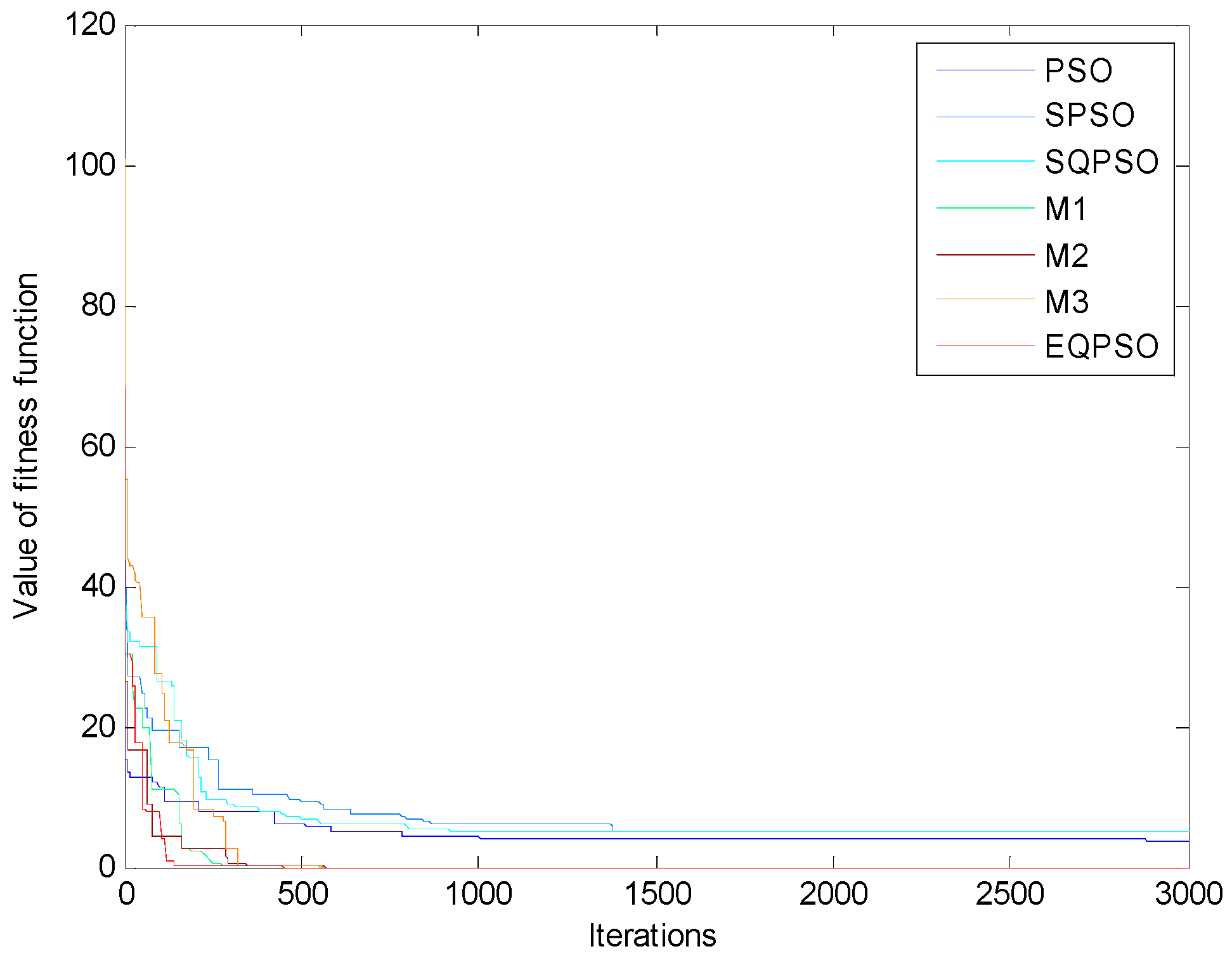
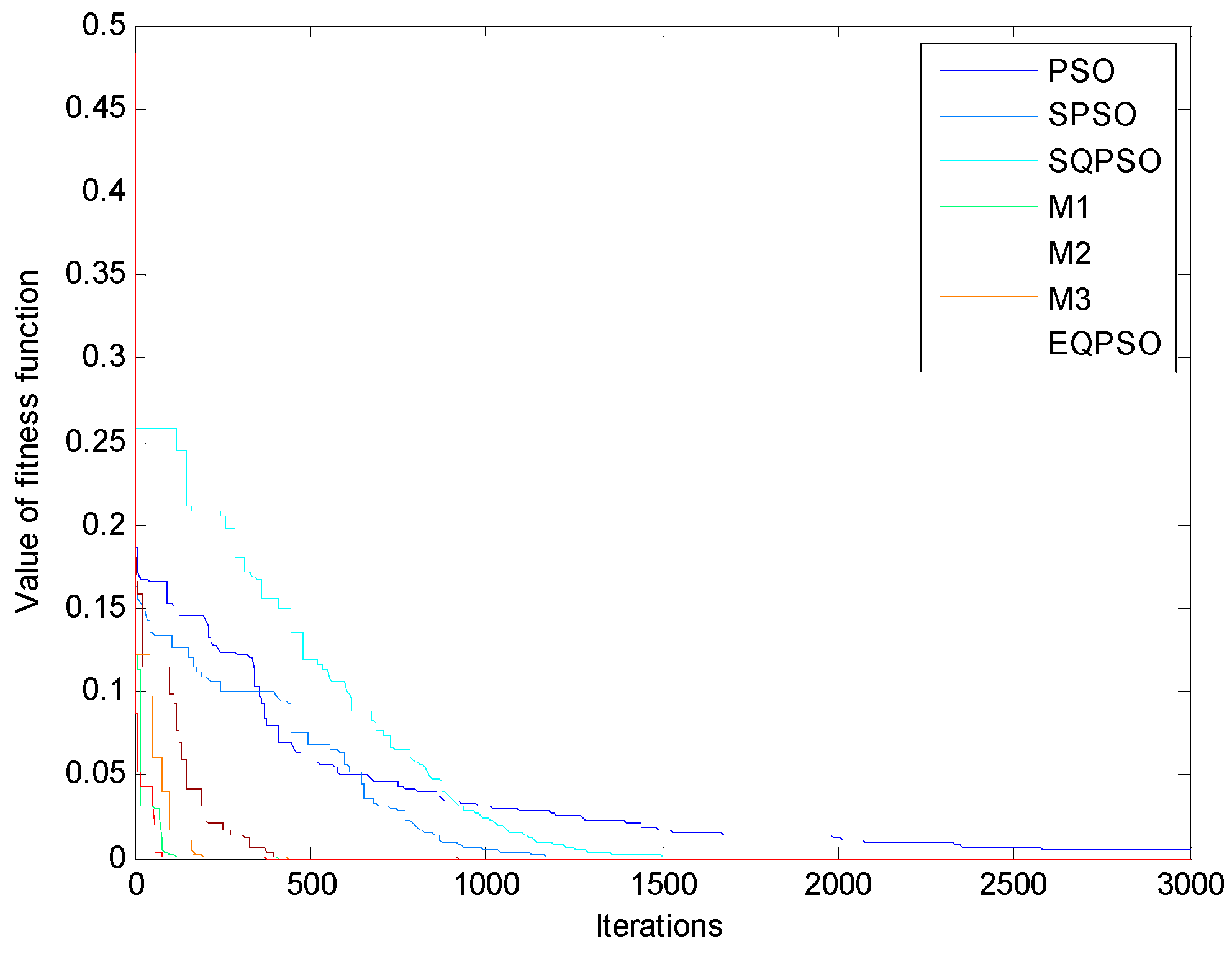
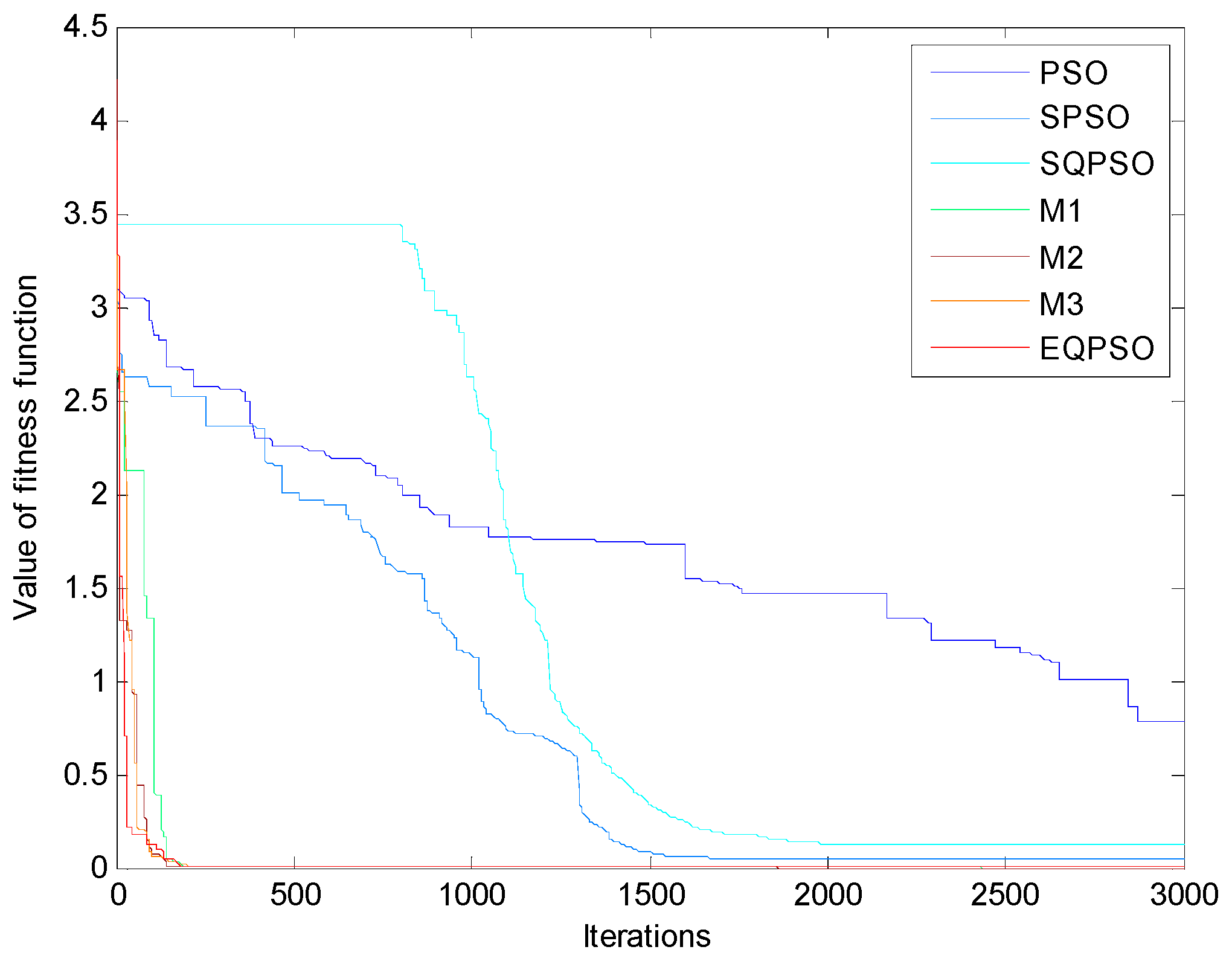
The convergence speeds of different optimization algorithms are shown in Figure 4, Figure 5, Figure 6 and Figure 7 (the swarm size was 80 and the number of iterations was 3000) when used to optimize the Sphere Model, Generalized Rastrigin, Griewank and Ackley functions. It can be found that the convergence speed of EQPSO is faster than other considered PSO methods.
Figure 4. Convergence speed of different PSO algorithms when used to optimize the Sphere Model function.
Information 06 00633 g004
Figure 5. Convergence speed of different PSO algorithms when used to optimize the Generalized Rastrigin function.
Information 06 00633 g005
Figure 6. Convergence speed of different PSO algorithms when used to optimize the Griewank function.
Information 06 00633 g006
Figure 7. Convergence speed of different PSO algorithms when used to optimize the Ackley function.
Information 06 00633 g007
EQPSO and the other considered PSO methods were also used to optimize the problems with constraints, and three functions with constraints of paper [26] (g07, g09 and g10, which are shown in Table 9) are used as the test functions.
Table 9. Test functions with constraints.
FunctionsMathematical ExpressionGlobal Minimum
g07 f 8 ( x ) = x 1 2 + x 2 2 + x 1 x 2 14 x 1 16 x 2 + ( x 3 10 ) 2 + 4 ( x 4 5 ) 2 + ( x 5 3 ) 2 + 2 ( x 6 1 ) 2 + 5 x 7 2 + 7 ( x 8 11 ) 2 + 2 ( x 9 10 ) 2 + ( x 10 7 ) 2 + 45 subject to: g 1 ( x ) = 105 + 4 x 1 + 5 x 2 3 x 7 + 9 x 8 0 g 2 ( x ) = 10 x 1 8 x 2 17 x 7 + 2 x 8 0 g 3 ( x ) = 8 x 1 + 2 x 2 + 5 x 9 2 x 10 12 0 g 4 ( x ) = 3 ( x 1 2 ) 2 + 4 ( x 2 3 ) 2 + 2 x 3 2 7 x 4 120 0 g 5 ( x ) = 5 x 1 2 + 8 x 2 + ( x 3 6 ) 2 2 x 4 40 0 g 6 ( x ) = x 1 2 + x ( x 2 2 ) 2 2 x 1 x 2 + 14 x 5 6 x 6 0 g 7 ( x ) = 0.5 ( x 1 8 ) 2 + 2 ( x 2 4 ) 2 + 3 x 5 2 x 6 30 0 g 8 ( x ) = 3 x 1 + 6 x 2 + 12 ( x 9 8 ) 2 7 x 10 0 where  10 x i 10   ( i = 1 , 2 , , 10 ) min ( f 8 ) = f 8 ( 2.171996 , 2.363683 , 8.773926 , 5.095984 , 0.9906548 , 1.430574 , 1.321644 , 9.828726 , 8.280092 , 8.375927 ) = 24.3062091
g09 f 9 ( x ) = ( x 1 10 ) 2 + 5 ( x 2 12 ) 2 + x 3 4 + 3 ( x 4 11 ) 2 + 10 x 5 6 + 7 x 6 2 + x 7 4 4 x 6 x 7 10 x 6 8 x 7 subject to: g 1 ( x ) = 127 + 2 x 1 2 + 3 x 2 4 + x 3 + 4 x 4 2 + 5 x 5 0 g 2 ( x ) = 282 + 7 x 1 + 3 x 2 + 10 x 3 2 + x 4 x 5 0 g 3 ( x ) = 196 + 23 x 1 + x 2 2 + 6 x 6 2 8 x 7 0 g 4 ( x ) = 4 x 1 2 + x 2 2 3 x 1 x 2 + 2 x 3 2 + 5 x 6 11 x 7 0 where  10 x i 10   ( i = 1 , 2 , , 7 ) min ( f 9 ) = f 9 ( 2.330499 , 1.951372 , 0.4775414 , 4.365726 , 0.6244870 , 1.038131 , 1.594227 ) = 680.6300573
g10 f 10 ( x ) = x 1 + x 2 + x 3 suject to: g 1 ( x ) = 1 + 0.0025 ( x 4 + x 6 ) 0 g 2 ( x ) = 1 + 0.0025 ( x 5 + x 7 x 4 ) 0 g 3 ( x ) = 1 + 0.01 ( x 8 x 5 ) 0 g 4 ( x ) = x 1 x 6 + 833.33252 x 4 + 100 x 1 83333.333 0 g 5 ( x ) = x 2 x 7 + 1250 x 5 + x 2 x 4 1250 x 4 0 g 6 ( x ) = x 3 x 8 + 1250000 + x 3 x 5 2500 x 5 0 where  100 x 1 10000 ,   1000 x i 10000   ( i = 2 , 3 ) , 10 x i 1000   ( i = 4 , 5 , , 8 ) min ( f 10 ) = f 10 ( 579.19 , 1360.13 , 5109.92 , 182.0174 , 295.5985 , 217.9799 , 286.40 , 395.5979 ) = 7049.25
The mechanism proposed in paper [26] was adopted to help the considered PSO methods of this paper to solve the functions with constraints. This mechanism is used to select the leaders, and it is based both on the feasible solutions and on the fitness value of a particle. In this mechanism, when two feasible particles are compared, the particle which has the highest fitness value wins. If one particle is not feasible and the other one is feasible, then the feasible particle wins. If both particles are infeasible, the particle that has the lowest fitness value wins. The idea is to choose as a leader the particle that, even when infeasible, lies closer to the feasible region. More detailed information about this mechanism can be found in paper [18]. When the seven considered methods were used to optimize these three functions, the size of their particle swarm was 80, and the maximum number of iterations was 3000. The results are shown in Table 10.
Table 10. Optimized results of g07, g09 and g10 found by different PSO algorithms.
g07g09g10
PSO26.8630685.25117512.6585
25.4369684.52647058.5644
SPSO26.3571685.23557489.2385
25.3321682.87017056.6452
SQPSO26.9852685.78197498.3160
25.8752684.25117053.8519
M125.0162684.62387369.3470
24.6835681.00647056.0559
M225.1302685.66507396.5825
24.6973681.42747057.8687
M325.5647686.66527450.6183
25.1960682.26977059.7984
EQPSO24.4080681.53077145.6589
24.3090680.63317051.0049
We can find from Table 10 that the results found by EQPSO are better than other PSO methods for functions g07, g09 and g10.

3.2. Comparison of Different Optimization Algorithms

In this section, we compare EQPSO with CMA-ES, GA, KH, an enhanced KH of paper [21], MBO, HS and APOA. All these methods were used to optimize the test functions of Table 1. For GA, KH, an enhanced KH of paper [21] (denoted as KH-E), MBO, HS, APOA and EQPSO, the population size is 20 and the maximal value of iterations is 1000. Other parameters of each algorithm were as follows: CMA-ES: SIGMA is a parameter which can determine the initial coordinate wise standard deviations for the search, and we set SIGMA to one third of the initial search region. GA: the selecting function was stochastic uniform, the crossover function was Intermediate, and the mutation function was Gaussian. The crossover fraction was 0.8. KH-E: The setting of KH-E was the same as paper [21]. MBO: The BAR value was equal to the percentage of population for MBO, and we randomly divided the whole population into population1 and population2. HS: Harmony memory considering rate was 0.95 and pitch adjustment rate was 0.3. APOA: the value of phototropism operator was 0.1. All programs were run ten times, the best result and mean result were used to evaluate the eight methods, and the results are shown in Table 11.
Table 11. Optimization results of different optimization methods.
f1f2f3f4f5f6f7
CMA-ES1.3485×10−159.85010.00170.11552.62143.3525×10−102.5101×10⁻¹⁵
7.4881×10−163.97981.8874×10−153.2028×10−112.1760×10−143.4148×10−141.0652×10⁻¹⁵
GA4.353712.29780.19083.24534.59030.16964.3999
2.12497.60930.13682.91853.39343.2352×10−50.5610
KH2.59231.581020.54402.99021.91492.48763.6905
0.06520.024220.40871.17038.7010×10−51.65111.6508
KH-E0.00410.18292.42360.00271.2341×10−20.00270.1204
8.5871×10−64.5122×10−42.25481.1790×10−40.0410×10−101.5855×10−48.6122×10−4
MBO1.5505×102197.25501.7072×10212.91170.04418.2794×1054.7425×104
0.43311.110312.41890.00135.5036×10−50.003446.3762
APOA1.8645×1018.31886.6463×10−13.53944.5291×10−22.7639×10−11.1939×101
1.4024×1017.89424.6362×10−13.51403.3480×10−34.2181×10−31.0967×101
HS4.7139×10−23.76311.1711×1012.1087×1011.3010×10−12.3984×1025.4177×101
4.4334×10−21.82591.0330×1012.0906×1011.7142×10−22.07155.0345×101
EQPSO0003.5527×10−1502.5546×10−193.6340
0003.5527×10−1503.5873×10−310.0199
As we can see from Table 11, for function f7, the results found by CMA-ES are better than EQPSO, and other than that the results of EQPSO are better than other methods.

3.3. Statistical Test

Finally, the sign test, which is known as a statistical test method, was adopted to verify the significance of the results found by EQPSO. In this method, the overall performance of algorithms is based on number of cases on which an algorithm is the overall winner. A detailed introduction to the sign test can be seen in paper [27]. Table 12 shows the critical number of wins needed to achieve both α = 0.05 and α = 0.1 levels of significance. An algorithm is significantly better than another if it performs better on at least the cases presented in each row of Table 12.
Table 12. Critical values for sign test.
Cases56789101112
α = 0.05 567789910
α = 0.1 56677899
The minimum value of 10 test functions (including all functions of Table 1 and Table 9) found by PSO, SPSO, SQPSO, M1, M2, M3 and EQPSO (the size of particle swarm was 80 and the maximum number of iterations was 3000) were analyzed by sign test, and the results are shown in Table 13. The minimum value of 7 test functions (all functions of Table 1) found by CMA-ES, GA, KH, KH-E, MBO, APOA, HS and EQPSO were also analyzed by sign test, and the results are shown in Table 14.
Table 13. Results of sign test performed on EQPSO (different PSO algorithms).
EQPSOPSOSPSOSQPSOM1M2M3
wins101010101010
loses000000
Detected differences α = 0.05
Table 14. Results of sign test performed on EQPSO (different optimization algorithms).
EQPSOCMA-ESGAKHKH-EMBOAPOAHS
wins6777777
loses1000000
Detected differences α = 0.1 α = 0.05 α = 0.05 α = 0.05 α = 0.05 α = 0.05 α = 0.05
As we can see, in the α = 0.05 level EQPSO shows a significant improvement over the other six PSO methods, GA, KH, KH-E, MBO, APOA and HS. For CMA-ES, EQPSO shows a significant improvement in the α = 0.1 level.

4. Conclusions

The QPSO algorithm shows ideal performance in the aspects of search ability, convergence speed, solution accuracy and solving robustness. However, it cannot be guaranteed that the traditional QPSO can find the global optimum when the number of iterations is limited.
We propose a novel way of computing the local attractor of QPSO to improve the global searching ability of QPSO in this case. With this proposed computing way, we can guarantee the particles are diversiform at the early stage of iterations, and ensure good performance in local searching ability at the later stage of iterations. Results of the test functions have proved that the proposed method has better performance in global searching ability.
In this paper, we improve the optimization performance of EQPSO through controlling the iterative process, as one can find that the initial distribution of particles also influences the optimization ability of EQPSO. We will focus our research on finding an effective way to initialize the particles of EQPSO in our future studies, and we believe the optimization performance will be more ideal through this research.

Acknowledgments

This work is supported by Program for New Century Excellent Talents in University (No. (2013) 47), National Natural Science Foundation of China (Nos. 61372139, 61101233, 60972155), Fundamental Research Funds for the Central Universities (No. XDJK2015C073), Science and Technology personnel training program Fund of Chongqing (No. Cstc2013kjrc-qnrc40011) and Fundamental Research Funds for the Central Universities (No. SWU115009).

Author Contributions

Pengfei Jia wrote this paper; Shukai Duan provided the analysis results on the performance test of the proposed QPSO, and prepared most of the figures for the paper; Jia Yan was involved in all research activities, provided many valuable experimental results and offered valuable suggestions. All authors have discussed about and contributed to the manuscript. All authors have read and approved the final manuscript.

Conflicts of Interest

The authors declare no conflict of interest.

References

  1. Van den Bergh, F.; Engelbrecht, A.P. A new locally convergent particle swarm optimizer. In Proceedings of the IEEE International Conference on Systems, Man and Cybernetics, Hammamet, Tunisia, 6–9 October 2002; pp. 96–101.
  2. Van den Bergh, F. An Analysis of Particle Swarm Optimizers. Ph.D. Thesis, University of Pretoria, Pretoria, South Africa, 2001. [Google Scholar]
  3. Coelho, L.D.S. Gaussian quantum-behaved particle swarm optimization approaches for constrained engineering design problems. Expert Syst. Appl. 2010, 37, 1676–1683. [Google Scholar] [CrossRef]
  4. Ch, S.; Anand, N.; Panigrahi, B.K.; Mathur, S. Streamflow forecasting by SVM with quantum behaved particle swarm optimization. Neurocomputing 2012, 4, 18–23. [Google Scholar] [CrossRef]
  5. Liu, H.; Yang, G.; Song, G. MIMO radar array synthesis using QPSO with normal distributed contraction-expansion factor. Procedia Eng. 2011, 15, 2449–2453. [Google Scholar] [CrossRef]
  6. Sun, J.; Chen, W.; Fang, W.; Wun, X.; Xu, W. Gene expression data analysis with the clustering method based on an improved quantum-behaved Particle Swarm Optimization. Eng. Appl. Artif. Intell. 2012, 25, 376–391. [Google Scholar] [CrossRef]
  7. Mariani, V.C.; Duck, A.R.K.; Guerra, F.A.; Coelho, L.D.S.; Rao, R.V. A chaotic quantum-behaved particle swarm approach applied to optimization of heat exchangers. Appl. Therm. Eng. 2012, 42, 119–128. [Google Scholar] [CrossRef]
  8. Zou, H.; Liang, D.; Zeng, J.; Feng, L. Quantum-behaved particle swarm optimization algorithm for the reconstruction of fiber Bragg grating sensor strain profiles. Opt. Commun. 2012, 285, 539–545. [Google Scholar] [CrossRef]
  9. Shayeghi, H.; Shayanfar, H.A.; Jalilzadeh, S.; Safari, A. Tuning of damping controller for UPFC using quantum particle swarm optimizer. Energy Convers. Manag. 2010, 51, 2299–2306. [Google Scholar] [CrossRef]
  10. Jia, P.; Tian, F.; He, Q.; Fan, S.; Liu, J.; Yang, S.X. Feature Extraction of Wound Infection Data for Electronic Nose Based on a Novel Weighted KPCA. Sens. Actuators B Chem. 2014, 201, 555–566. [Google Scholar] [CrossRef]
  11. Jia, P.; Tian, F.; Fan, S.; He, Q.; Feng, J.; Yang, S.X. A novel sensor array and classifier optimization method of electronic nose based on enhanced quantum-behaved particle swarm optimization. Sen. Rev. 2014, 34, 304–311. [Google Scholar] [CrossRef]
  12. Kern, S.; Müller, S.D.; Hansen, N.; Büche, D.; Ocenasek, J.; Koumoutsakos, P. Learning probability distributions in continuous evolutionary algorithms-a comparative review. Nat. Comput. 2004, 3, 77–112. [Google Scholar] [CrossRef]
  13. Wang, G.; Gandomi, A.H.; Alavi, A.H.; Hao, G. Hybrid krill herd algorithm with differential evolution for global numerical optimization. Neural Comput. Appl. 2014, 25, 297–308. [Google Scholar] [CrossRef]
  14. Guo, L.; Wang, G.; Gandomi, A.H.; Alavi, A.H.; Duan, H. A new improved krill herd algorithm for global numerical optimization. Neurocomputing 2014, 138, 392–402. [Google Scholar] [CrossRef]
  15. Wang, G.; Guo, L.; Gandomi, A.H.; Hao, G.; Wang, H. Chaotic krill herd algorithm. Inf. Sci. 2014, 274, 17–34. [Google Scholar] [CrossRef]
  16. Wang, G.; Deb, S.; Cui, Z. Monarch butterfly optimization. Neural Comput. Appl. 2015. [Google Scholar] [CrossRef]
  17. Geem, Z.W.; Kim, J.H.; Loganathan, G.V. A new heuristic optimization algorithm: Harmony search. Simulation 2001, 76, 60–68. [Google Scholar] [CrossRef]
  18. Wang, G.; Gandomi, A.H.; Zhao, X.; Chu, H.C.E. Hybridizing harmony search algorithm with cuckoo search for global numerical optimization. Soft Comput. 2014, 1–13. [Google Scholar] [CrossRef]
  19. Yu, B.; Cui, Z.; Zhang, G. Artificial plant optimization algorithm with correlation branches. J. Bioinform. Intell. Control 2013, 2, 146–155. [Google Scholar] [CrossRef]
  20. Kennedy, J.; Elbert, R.C. Particle swarm optimization. In Proceedings of the IEEE International Conference on Neural Networks, Perth, WA, USA, 27 November–1 December 1995; pp. 1942–1948.
  21. Shi, Y.; Eberhart, R.C. A modified particle swarm optimizer. In Proceedings of the IEEE International Conference on Evolutionary Computation, Anchorage, AK, USA, 4–9 May 1998; pp. 69–73.
  22. Shi, Y.; Eberhart, R.C. Empirical study of particle swarm optimization. In Proceedings of the Congress on Evolutionary Computation, Washington, DC, USA, 6–9 July 2000; pp. 1945–1950.
  23. Sun, J.; Feng, B.; Xu, W. Particle swarm optimization with particles having quantum behavior. In Proceedings of the 2004 IEEE Congress on Evolutionary Computation, Portland, OR, USA, 19–23 June 2004; pp. 326–331.
  24. Xi, M.; Sun, J.; Xu, W. An improved quantum-behaved particle swarm optimization algorithm with weighted mean best position. Appl. Math. Comput. 2008, 205, 751–759. [Google Scholar] [CrossRef]
  25. Sun, J.; Fang, W.; Wu, X.; Xu, W. Quantum Particle Swarm Optimization: Principle and Application; Tsinghua University Press: Beijing, China, 2011. [Google Scholar]
  26. Pulido, G.T.; Coello, C.A. A constraint-handing mechanism for particle swarm optimization. In Proceeding of the 2004 IEEE Congress on Evolutionary Computation, Portland, OR, USA, 19–23 June 2004; pp. 1396–1403.
  27. Derrac, J.; Garcia, S.; Molina, D.; Herrera, F. A practical tutorial on the use of nonparametric statistical as a methodology for computing evolutionary and swarm intelligence algorithm. Swarm Evolut. Comput. 2011, 1, 3–18. [Google Scholar] [CrossRef]

