On Solving the Fuzzy Customer Information Problem in Multicommodity Multimodal Routing with Schedule-Based Services

Abstract

In this study, we combine the fuzzy customer information problem with the multicommodity multimodal routing with schedule-based services which was explored in our previous study [1]. The fuzzy characteristics of the customer information are embodied in the demanded volumes of the multiple commodities and the time windows of their due dates. When the schedule-based services are considered in the routing, schedule constraints emerge because the operations of block container trains should follow their predetermined schedules. This will restrict the routes selection from space-time feasibility. To solve this combinatorial optimization problem, we first build a fuzzy chance-constrained nonlinear programming model based on fuzzy possibility theory. We then use a crisp equivalent method and a linearization method to transform the proposed model into the classical linear programming model that can be effectively solved by the standard mathematical programming software. Finally, a numerical case is presented to demonstrate the feasibility of the proposed method. The sensitivity of the best solution with respect to the values of the confidence levels is also examined.

1. Introduction

The routing problem has always been a highlight in combinatorial optimizations. Great importance has been attached to it, not only in the transportation field, but also in many other industries such as telecommunications, manufacturing and the Internet [2]. The routing problem aims at improving the performance of a system by reasonably distributing the flow of the object (data, signal or products) in it. As for the multimodal routing problem, it is defined as selecting the best routes to move commodities from their origins to their destinations through a multimodal service network. The multimodal routing problem arises under the following conditions.

The remarkable growth of international trade in recent years stimulates the worldwide commodity circulation, which significantly expands the geographical scale of the transportation network, extends the freight transportation distance, and leads to a more complex transportation environment. All these tendencies present great challenges for decision makers from various aspects including transportation cost, efficiency, reliability and so on. Meanwhile, because of the integrative combination of the respective advantages of different transportation service modes, multimodal transportation has been proved to be a more cost-efficient [3] and environment-friendly [4] means compared with the traditional uni-modal transportation in a long-haul transportation setting. Therefore, large numbers of enterprises decide to adopt multimodal transportation schemes to transport their products or materials. According to the relevant statistics, the volume fulfilled by the multimodal transportation accounts for 80% of the total freight volume in North America [5]. However, the logistics cost is still high, and accounts for approximately 30%–50% of the total production cost of enterprises [6]. Consequently, lowering transportation costs by advanced multimodal routing becomes an effective approach for enterprises to raise profits and maintain competitiveness in the global market [2].

By considering the practical demand of lowering the transportation costs by selecting the best multimodal routes, many researchers have devoted themselves to the multimodal routing problem (or intermodal routing problem) in recent decades. Barnhart and Ratliff [7] developed a foundational framework on modeling intermodal routing, and introduced a solution procedure with matching to solve the routing problem from Cincinnati to Atlanta/Chattanooga. Boardman et al. [8] designed a real-time intermodal routing decision support system by incorporating the k-shortest path double-swap method with database and user interface. Lozano and Storchi [9], Lam and Srikanthan [10] and Boussedjra et al. [11] highlighted the intermodal/multimodal shortest path problem. They separately developed an ad hoc modified chronological algorithm, clustering technique accelerated k-shortest algorithm and multi-label label correcting shortest path algorithm, to identify the shortest path in the intermodal/multimodal service network. Zhang and Guo [12] described the physical structure of the multimodal service network, and proposed a foundational network assignment model for the multimodal routing problem. Zhang et al. [13] formulated the multimodal routing problem as a generalized shortest path problem, built a 0–1 integer programming model based on Reddy and Kasilingam’s work [14], and adopted Dijkstra algorithm to obtain the optimal solution of the model. Winebrake et al. [15] developed a geospatial model to find optimal routes with different objectives in the intermodal transportation network. The construction and solution of the model were implemented by ArcGIS software. Kim et al. [16] and Chang et al. [17] both analyzed the intermodal sea–truck routing problem for container transportation in South Korea, and formulated classical programming models to solve the empirical cases in South Korea. The proposed models were solved by standard mathematical programming software. Liu et al. [18] explored the dynamic path optimization for multimodal service network. The network deformation method was used in their study to transform the initial network into a directed simple graph. This enabled the problem to be effectively solved by a modified Dijkstra algorithm. Cho et al. [19] presented a weighted constrained shortest path model and a label setting algorithm to draw the optimal international intermodal routing. They applied the proposed method to a real-world routing case from Busan to Rotterdam. Sun and Lang [20] as well as Xiong and Wang [21] separately discussed the bi-objective optimization for the multimodal routing problem that aims at minimizing transportation costs and transportation time. The normalized normal constraint method and Taguchi genetic algorithm were utilized to generate the Pareto frontier of the problem. The former also conducted a sensitivity analysis of the Pareto frontier with respect to demand and supply.

Above all, substantial accomplishments have been achieved in the multimodal routing problem. However, some research potential still exists.

(1) The majority of the current studies concentrated on the single commodity flow routing problem. In practice, decision makers usually need to plan routes for multiple commodities in their planning horizons. In addition, the best routing for multiple commodities is not the simple set of the respective independent best routes for all commodities, because the multimodal service network is usually capacitated. Therefore, it is necessary to combine the multicommodity flow with the multimodal routing.

(2) In the current studies, rail schedules are rarely considered in the model formulation. Many studies, especially the domestic ones, formulated the rail service as a time-flexible pattern that is similar to the road service, and hence simplified the connection between different transportation services in the terminals as a continuous “arrival-transshipment-departure” procedure. Actually, rail services are organized by predetermined schedules, especially in China, and train schedules will restrict the routing because of space-time feasibility. If the transportation of a commodity along a route cannot match the schedules of the rail services on it, the planned route is infeasible in the practice. Consequently, consideration of schedules in routing modeling is quite worthwhile.

(3) Multimodal routing in most current studies was oriented on the certain customer information, which means all customer information is determined and known when making routing decisions. However, as has been claimed in many studies as well as indicated in the practice, customer information, especially their demands, is difficult to determine during the planning period. Many studies on other transportation problems, e.g., the vehicle routing problem [22,23,24] and service network design problem [25,26], have all paid great attention to the uncertain issues from the fuzzy or stochastic viewpoint. Hence uncertain customer information is also a characteristic that should not be neglected in the multimodal routing problem.

The first two issues above have already been explored in our previous study (see Reference [1]). In this study, we will focus on integrating the fuzzy customer information problem into this previous study in order to develop the initial problem into its extended version: schedule-constrained multicommodity multimodal routing problem with fuzzy customer information.

Similar to the transportation scenario constructed in Reference [1], the rail service (the schedule-based service) in the multimodal service network specifically refers to the “point-to-point” block container train service. This kind of service is operated directly and periodically from its loading organization station to its unloading organization station. For the convenience of modeling, the same block container train in different periods is treated as a different one. The road service is formulated as an uncapacitated time-flexible service, which matches the superiority of the road service (container trucks) in its organization flexibility. Transshipment is not necessary when the commodity arrives at and then departs from a terminal by road service, and a road service route can be covered entirely or partly in the routing. For the convenience of modeling, a road service can be divided into several segments, e.g., a directed road service route (g, h, i, j) is divided into sub segments (g, h), (g, i), (g, j), (h, i), (h, j), and (i, j).

For the convenience of readability, we briefly introduce the schedule Constraints (1)–(4) resulting from the actual transportation practice that the operation of block container trains should follow their predetermined schedules. For detailed relative information, we can refer to Reference [1].

(1) If the commodity plans to be moved by rail service from the current terminal (loading organization station) to the successor terminal (unloading organization station), its arrival time at the current terminal should not be later than the upper bound of the loading operation time window of the block container train at the same terminal.

(2) In the above situation, if the arrival time of the commodity at the terminal is earlier than the lower bound of the operation time window of the block container train at the same terminal, it should wait until the lower bound of the time window.

(3) After being loaded on the train, the commodity should wait until the departure time of the train. Then it departs from the current terminal to the successor terminal, and arrives at the successor terminal at the arrival time of the train.

(4) The commodity should wait until the lower bound of the unloading operation time window of the train at the successor terminal, and then gets unloaded from it.

For the uncertain customer information problem, we will explain it in detail by using a whole section. After defining the symbols that will be used in the model formulation (Section 2), we organize the remaining sections of this study as follows. In Section 3, we analyze the uncertain characteristics of the customer information from the fuzzy viewpoint, and propose fuzzy demands and fuzzy soft due date time windows to define the uncertainty. In Section 4, a fuzzy chance-constrained nonlinear programming model for the routing problem is established based on fuzzy possibility theory. In Section 5, we introduce a crisp equivalent method and a linearization method to transform the proposed model into its equivalent linear programming form, after which the routing problem can be effectively solved by the standard mathematical programming software. In Section 6, a numerical case is presented to demonstrate the feasibility of the proposed model, and the sensitivity of the best solution with respect to the values of the confidence levels is also examined. Finally, conclusions of this study are drawn in Section 7.

2. Notations

N: terminal set in the multimodal service network, h, i, and j are the terminal indexes;

A: directed transportation arc set in the multimodal service network, and $A=$$\left\{\left(i,j\right)|i\in N,j\in N\right\}$;

K: commodity set, and k is the commodity index;

${\Gamma }_{ij}$: set of rail services on (i, j);

${\Omega }_{ij}$: set of road services on (i, j);

S: transportation service set in the multimodal service network, s and r are the service indexes, $S={\displaystyle {\cup }_{\left(i,j\right)\in A}\left\{S_{ij}\right\}}$ where $S_{ij}$ is transportation service set on (i, j), and $S_{ij}={\Gamma }_{ij}\cup {\Omega }_{ij}$;

${\delta }^{-}\left(i\right)$: predecessor terminal set to terminal i, and ${\delta }^{-}\left(i\right)\subseteq N$;

${\delta }^{+}\left(i\right)$: successor terminal set to terminal i, and ${\delta }^{+}\left(i\right)\subseteq N$;

$o_k$: origin terminal of commodity k;

$d_k$: destination terminal of commodity k;

$t_{release}^k$: release time of commodity k from its origin terminal;

$\left[l_i^s,u_i^s\right]$: loading/unloading operation time window of rail service s at terminal i;

$S{D}_i^s$, $S{A}_j^s$: scheduled departure time and scheduled arrival time of service s from terminal i and at terminal j on (i, j);

$Q_{ij}^s$: available carrying capacity of rail service s at terminal i, unit: TEU;

$t_{ijs}$: transportation time of service s on (i, j), especially for $s\in {\Gamma }_{ij}$, the effective transportation time $t_{ijs}=l_i^s-S{D}_i^s$, unit: h;

$c_{ij}^s$: unit transportation costs of by service s on (i, j), unit: ¥/TEU;

$c_s$: unit loading/unloading operation costs of service s, unit: ¥/TEU;

$c_{store}$: unit inventory costs of rail service s, unit: ¥/TEU-h;

$c_{pick}$: additional charges for picking up the unit commodity from shipper at a rail terminal by rail service at origin, unit: ¥/TEU;

${\varphi }_k$: a 0-1 indicating parameter, if the above service is demanded, ${\varphi }_k$ = 1, otherwise ${\varphi }_k$ = 0;

$c_{delivery}$: additional charges for delivering the unit commodity from rail terminal to receiver by rail service at destination, unit: ¥/TEU;

${\mu }_k$: a 0-1 indicating parameter, if the above service is demanded, ${\mu }_k$ = 1, otherwise ${\mu }_k$ = 0;

π: inventory period free of charge, unit: h;

M: a large enough positive number;

$X_{ijs}^k$: 0-1 variable, If commodity k is moved on (i, j) by service s, $X_{ijs}^k$ = 1, otherwise $X_{ijs}^k$ = 0 (decision variable);

$Y_i^k$: arrival time of commodity k at terminal i (decision variable);

$Z_{ijs}^k$: charged inventory time at terminal i before being moved on (i, j) by rail service s, unit: h (decision variable).

3. Fuzzy Characteristics of the Customer Information

3.1. Fuzzy Demanded Volume

It is difficult to master the accurate demand information of the customers when planning the best multimodal routes in advance. On the one hand, the planning is earlier than the actual transportation; and, on the other hand, due to the impact of many uncertain factors in production and consumption, the demands (measured by demanded volumes of the commodities) negotiated by shippers and receivers are difficult to be determined during the planning period. Consequently, there is a great challenge for the decision makers in that the demands are uncertain before the actual transportation starts. The advance routing should deal with this uncertainty. Generally, there is not enough historical data that can be utilized to fit the probability distributions for all the uncertain demands, but the decision makers can effectively estimate the demands according to their expertise. Therefore, when the stochastic demands are unattainable, it is worthwhile to adopt fuzzy logic to estimate the uncertainty of the demands.

In this study, we use a triangular fuzzy number to represent the demanded volume of a commodity flow. For commodity k, its fuzzy volume is defined as:

$$\widetilde{q_k}=\left(q_k^L,q_k^M,q_k^U\right)\forall k\in K$$

where $q_k^L$<$q_k^M$<$q_k^U$, and $q_k^M$ is the most likely volume of commodity k.

Consequently, the total volume of commodities loaded on a block container train is:

$$V_{ijs}={\displaystyle \sum _{k\in K}\widetilde{q_k}\cdot X_{ijs}^k}\forall \left(i,j\right)\in A,\forall s\in {\Gamma }_{ij}$$

$V_{ijs}$ is also a triangular fuzzy number according to the fuzzy arithmetic rules, and can be rewritten as:

$$\widetilde{V_{ijs}}=\left({\displaystyle \sum _{k\in K}{q}_k^L\cdot X_{ijs}^k},{\displaystyle \sum _{k\in K}{q}_k^M\cdot X_{ijs}^k},{\displaystyle \sum _{k\in K}{q}_k^U\cdot X_{ijs}^k}\right)=\left(V_{ijs}^L,V_{ijs}^M,V_{ijs}^U\right)\forall \left(i,j\right)\in A,\forall s\in {\Gamma }_{ij}$$

3.2. Fuzzy Soft Time Window

Due date is closely related to the customer satisfaction level. It can be a time point or a time window. In general, a customer considers that the transportation service is satisfactory when the arrival time of the commodity at the destination is neither too early nor too late. Therefore, time windows are more suitable than time points to represent the due dates of moving commodities. Moreover, in practice, customers also accept violation of the time windows to some degree. In that case, the satisfaction level of the customer will decrease when the violation degree increases. Therefore, the time windows in this study are soft ones instead of hard ones that stress the arrival time of a commodity at its destination must be within the time window.

The customers may consider “good” if the arrival time at the destination is within the time window, while “all right” or “bad” or other personal human feelings if the arrival time is out of the range of the time window [24]. Hence, we can use trapezoidal fuzzy numbers to represent the due date, and further measure the customer satisfaction quantitatively using the fuzzy membership function [27,28]. For commodity k, its due date is defined as:

$$\widetilde{T_k}=\left(T_k^{min},T_k^L,T_k^U,T_k^{max}\right)\forall k\in K$$

where $T_k^{min}$<$T_k^L$<$T_k^U$<$T_k^{max}$, and [$T_k^L$,$T_k^U$] is the time window that the customer considers the arrival time of the commodity at the destination to be neither too early nor too late. The corresponding satisfaction level in the fuzzy soft time window is shown in Figure 1.

The membership function of the time window is as Equation (1), where ${\mu }_k\left(Y_{d_k}^k\right)$ is also the customer satisfaction level when commodity k arrives at its destination $d_k$ at $Y_{d_k}^k$.

$${\mu }_k\left(Y_{d_k}^k\right)=\{\begin{array}{c}\frac{Y_{d_k}^k-T_k^{min}}{T_k^L-T_k^{min}},T_k^{min}\le Y_{d_k}^k<T_k^L\\ 1,T_k^L\le Y_{d_k}^k\le T_k^U\\ \frac{Y_{d_k}^k-T_k^{max}}{T_k^U-T_k^{max}},T_k^U<Y_{d_k}^k\le Y_k^{max}\\ 0,otherwise\end{array}\forall k\in K$$

(1)

Assuming that the customer satisfaction level should not be lower than the confidence level γ (γ∈[0, 1]), the acceptable arrival time at the destination ranges from $\left[\left(T_k^L-T_k^{min}\right)\cdot \gamma +T_k^{min}\right]$ to $\left[\left(T_k^U-T_k^{max}\right)\cdot \gamma +T_k^{max}\right]$.

4. Model Formulation

The schedule-constrained multicommodity multimodal routing problem aims to select the best time-feasible routes for all commodity flows through the multimodal service network. Oriented on the customers’ practical demand of lowering the total transportation costs, minimizing the generalized costs of all commodities is therefore set as the optimization objective. The generalized costs include transportation costs en route, loading/unloading operation costs and inventory costs at terminals, as well as the customer-specific additional rail origin-pickup/destination-delivery service costs. First, we formulate this problem as a nonlinear programming model with fuzzy parameters (M1). The framework of M1 derives from the model in Reference [1].

• Objective Function:

  $$minimize{\displaystyle \sum _{k\in K}\widetilde{q_k}\cdot {\displaystyle \sum _{\left(i,j\right)\in A}{\displaystyle \sum _{s\in S_{ij}}{c}_{ij}^s\cdot X_{ijs}^k}}}$$

  (2)

  $$+{\displaystyle \sum _{k\in K}\widetilde{q_k}\cdot {\displaystyle \sum _{i\in N}\left({\displaystyle \sum _{h\in {\delta }^{-}\left(i\right)}{\displaystyle \sum _{r\in S_{hi}}{c}_r\cdot X_{hir}^k}}+{\displaystyle \sum _{j\in {\delta }^{+}\left(i\right)}{\displaystyle \sum _{s\in S_{ij}}{c}_s\cdot X_{ijs}^k}}\right)}}$$

  (3)

  $$+{\displaystyle \sum _{k\in K}\widetilde{q_k}\cdot {\displaystyle \sum _{\left(i,j\right)\in A}{\displaystyle \sum _{s\in {\Gamma }_{ij}}{c}_{store}\cdot Z_{o_{k}js}^k}}}$$

  (4)

  $$+{\displaystyle \sum _{k\in K}\widetilde{q_k}\cdot {\varphi }_k\cdot {\displaystyle \sum _{j\in {\delta }^{+}\left(o_k\right)}{\displaystyle \sum _{s\in {\Gamma }_{o_{k}j}}{c}_{pick}\cdot X_{o_{k}js}^k}}}+{\displaystyle \sum _{k\in K}\widetilde{q_k}\cdot {\mu }_k\cdot {\displaystyle \sum _{j\in {\delta }^{-}\left(d_k\right)}{\displaystyle \sum _{s\in {\Gamma }_{{id}_k}}{c}_{delivery}\cdot X_{i{d}_{k}s}^k}}}$$

  (5)
• Subject to:

  $${\displaystyle \sum _{j\in {\delta }^{+}\left(i\right)}{\displaystyle \sum _{s\in S_{ij}}{X}_{ijs}^k}}-{\displaystyle \sum _{h\in {\delta }^{-}\left(i\right)}{\displaystyle \sum _{r\in S_{hi}}{X}_{hir}^k}}=\{\begin{array}{c}1,i=o_k\\ 0,\forall i\in N\backslash \left\{o_k,d_k\right\}\\ -1,i=d_k\end{array}\forall k\in K,\forall i\in N$$

  (6)

  $${\displaystyle \sum _{s\in S_{ij}}{X}_{ijs}^k}\le 1\forall k\in K,\forall \left(i,j\right)\in A$$

  (7)

  $$\widetilde{V_{ijs}}\le Q_{ij}^s\forall \left(i,j\right)\in A,\forall s\in {\Gamma }_{ij}$$

  (8)

  $$Y_{o_k}^k=t_{release}^k\forall k\in K$$

  (9)

  $$\left(max\left\{Y_i^k,S{D}_i^s\right\}+t_{ijs}-Y_j^k\right)\cdot X_{ijs}^k=0\forall k\in K,\forall \left(i,j\right)\in A,\forall s\in S_{ij}$$

  (10)

  $$Y_i^k\le u_i^s\cdot X_{ijs}^k+M\left(1-X_{ijs}^k\right)\forall k\in K,\forall \left(i,j\right)\in A,\forall s\in {\Gamma }_{ij}$$

  (11)

  $${\mu }_k\left(Y_{d_k}^k\right)\ge \gamma \forall k\in K$$

  (12)

  $$\left(max\left\{0,l_i^s-Y_i^k-\pi \right\}-Z_{ijs}^k\right)\cdot X_{ijs}^k=0\forall k\in K,\forall \left(i,j\right)\in A,\forall s\in {\Gamma }_{ij}$$

  (13)

  $$X_{ijs}^k\in \left\{0,1\right\}\forall k\in K,\forall \left(i,j\right)\in A,\forall s\in S_{ij}$$

  (14)

  $$Y_i^k\ge 0\forall k\in K,\forall i\in N$$

  (15)

  $$Z_{ijs}^k\ge 0\forall k\in K,\forall \left(i,j\right)\in A,\forall s\in {\Gamma }_{ij}$$

  (16)

Equations (2)–(5) are the transportation costs en route, loading and unloading costs at terminals, inventory costs at terminal as well as the rail origin-pickup and destination-delivery service costs, respectively. Their summation is the generalized costs that the decision maker plans to minimize.

Constraint Set (6) are the commodity flow conservation equation. Constraint Sets (6) and (7) ensure the integrity of each commodity flow that one and only one route can be selected to move the commodity through the multimodal service network. Constraint Set (8) is the capacity constraint resulting from the limited available carrying capacity of a block container train. Constraint Set (9) assumes the arrival time of the commodity at its origin equals its release time. Constraint Set (10) ensures the compatibility requirements between decision variables $X_{ijs}^k$ and $Y_j^k$. Constraint Set (11) ensures the arrival time of the commodity at a terminal will not exceed the upper bound of the operation time window of the utilized block container train at the same terminal. Constraint Set (12) is the customer satisfaction level constraint. Constraint Set (13) is similar to Constraint Set (10), and ensures the compatibility requirements among decision variables $X_{ijs}^k$, $Y_i^k$ and $Z_{ijs}^k$. Constraint Sets (14)–(16) are variable domain constraints.

In M1, the Objective Function (2)–(5) and Constraint Set (8) are involved with fuzzy parameters, the mathematical meaning of minimizing the objective and of the constraint are hence not clear, consequently M1 is not a well-defined model. In order to obtain a well-defined model, we need to transform the fuzzy objective and the fuzzy constraint set into their respective crisp equivalents. Based on Liu and Iwamura’s theoretical framework on chance-constrained programming in a fuzzy environment [29], we can obtain M1’s crisp equivalent fuzzy chance-constrained programming model (M2) as follows. (M2 is a well-defined model.)

• Objective Function:

  $$minimize\overline{f}$$

  (17)
• Subject to:

  $$Pos\left\{f\left(X,Y,Z,\tilde{q}\right)\le \overline{f}\right\}\ge \alpha$$

  (18)

  $$Pos\left\{\widetilde{V_{ijs}}\le Q_{ij}^s\right\}\ge \beta \forall \left(i,j\right)\in A,\forall s\in {\Gamma }_{ij}$$

  (19)

Constraint Sets (6), (7), and (9)–(16).

In M2, $Pos\left\{\cdot \right\}$ denotes the possibility of the event in $\left\{\cdot \right\}$ [29]. $\alpha$ and $\beta$ are predetermined confidence levels that indicate the decision maker’s subjective preference for the corresponding issues, and $\alpha$, $\beta$∈[0, 1]. $f\left(X,Y,Z,\tilde{q}\right)$ is the objective value of M1 where $X={\displaystyle {\cup }_{k\in K,\left(i,j\right)\in A,s\in S_{ij}}\left\{X_{ijs}^k\right\}}$, $Y={\displaystyle {\cup }_{k\in K,i\in N}\left\{Y_i^k\right\}}$, $Z={\displaystyle {\cup }_{k\in K,\left(i,j\right)\in A,s\in {\Gamma }_{ij}}\left\{Z_{ijs}^k\right\}}$ and $\tilde{q}={\displaystyle {\cup }_{k\in K}\left\{\widetilde{q_k}\right\}}$. For $\forall \left(X,Y,Z\right)$, $f\left(X,Y,Z,\tilde{q}\right)$ is also a triangular fuzzy number based on the fuzzy arithmetic rules. When confidence level $\alpha$ is given, there possibly exist several potential $\overline{f}$ that satisfy Constraint Set (18). Minimizing $\overline{f}$ as the objective of M2 will find the minimal value (min$\overline{f}$) of $f\left(X,Y,Z,\tilde{q}\right)$ with confidence level $\alpha$. Constraint Set (19) means the possibility that the total volume of commodities loaded on a block container train do not exceed its available carrying capacity should not be lower than the given confidence level $\beta$.

5. Solution Strategy

M2 is a fuzzy chance-constrained nonlinear programming model. Because of the restrictions of the fuzzy chance constraint sets and the nonlinear constraint sets, it is difficult to solve this by the exact solution algorithm that can be effectively implemented by the standard mathematical software. Therefore, it is necessary to conduct some transformations to M2. It is obvious that the problem will be effectively solvable if M2 can be transformed into a linear programming model. For this purpose, we conduct the following transformations to M2 successively.

5.1. Crisp Equivalent of the Fuzzy Chance Constraint Sets

We consider a general triangular fuzzy number $\tilde{a}=\left(a^L,a^M,a^U\right)$ where $a^L$>$a^M$>$a^U$>0, let ${\mu }_{\tilde{a}}\left(x\right)$ denote its membership function whose expression is as Equation (20).

$${\mu }_{\tilde{a}}\left(x\right)=\{\begin{array}{c}\frac{x-a^L}{a^M-a^L},a^L\le x\le a^M\\ \frac{a^U-x}{a^U-a^M},a^M\le x\le a^U\\ 0,otherwise\end{array}$$

(20)

The definition of $Pos\left\{\tilde{a}\le b\right\}$ is as [29]: $Pos\left\{\tilde{a}\le b\right\}=sup\left\{{\mu }_{\tilde{a}}\left(x\right)|x\in R,x\le b\right\}$.

Lemma: 

$\forall \tilde{a}=\left(a^L,a^M,a^U\right)$, for any predetermined confidence level $\lambda$∈[0, 1], $Pos\left\{\tilde{a}\le b\right\}\ge \lambda$ if and only if $b\ge \left(1-\lambda \right)\cdot a^L+\lambda \cdot a^M$.

Proof: 

First we prove $Pos\left\{\tilde{a}\le b\right\}\ge \lambda \Rightarrow b\ge \left(1-\lambda \right)\cdot a^L+\lambda \cdot a^M$ (sufficiency), and the proof is also illustrated by Figure 2.

$$\begin{array}{l}\begin{array}{c}Pos\left\{\tilde{a}\le b\right\}\ge \lambda \Rightarrow sup\left\{{\mu }_{\tilde{a}}\left(x\right)|x\in R,x\le b\right\}\ge \lambda \Rightarrow b\ge x^{*}\\ \frac{x^{*}-a^L}{a^M-a^L}=\lambda \Rightarrow x^{*}=\left(a^M-a^L\right)\cdot \lambda +a^L\end{array}\}\Rightarrow b\ge \left(a^M-a^L\right)\cdot \lambda +a^L\\ \Rightarrow b\ge \left(1-\lambda \right)\cdot a^L+\lambda \cdot a^M.\end{array}$$

Then we prove $b\ge \left(1-\lambda \right)\cdot a^L+\lambda \cdot a^M\Rightarrow Pos\left\{\tilde{a}\le b\right\}\ge \lambda$ (necessity), and the proof is also illustrated by Figure 3.

If $a^M\le b$, $sup\left\{{\mu }_{\tilde{a}}\left(x\right)|x\in R,x\le b\right\}=1\Rightarrow Pos\left\{\tilde{a}\le b\right\}=1\Rightarrow Pos\left\{\tilde{a}\le b\right\}\ge \lambda$.

If $a^M>b$, $\begin{array}{c}sup\left\{{\mu }_{\tilde{a}}\left(x\right)|x\in R,x\le b\right\}={\mu }_{\tilde{a}}\left(b\right)=\frac{b-a^L}{a^M-a^L}\Rightarrow Pos\left\{\tilde{a}\le b\right\}=\frac{b-a^L}{a^M-a^L}\\ b\ge \left(1-\lambda \right)\cdot a^L+\lambda \cdot a^M\Rightarrow \frac{b-a^L}{a^M-a^L}\ge \lambda \end{array}\}\Rightarrow Pos\left\{\tilde{a}\le b\right\}\ge \lambda$.

Above all, the proposed lemma is proven.

According to the lemma above, the crisp equivalent of fuzzy chance Constraint Set (18) is:

$$\overline{f}\ge \left(1-\alpha \right)\cdot {\displaystyle \sum _{k\in K}{q}_k^L\cdot {\omega }_k}+\alpha \cdot {\displaystyle \sum _{k\in K}{q}_k^M\cdot {\omega }_k}$$

(21)

where ${\omega }_k$ represents the following function.

$$\begin{array}{l}{\displaystyle \sum _{\left(i,j\right)\in A}{\displaystyle \sum _{s\in S_{ij}}{c}_{ij}^s\cdot X_{ijs}^k}}+{\displaystyle \sum _{i\in N}\left({\displaystyle \sum _{h\in {\delta }^{-}\left(i\right)}{\displaystyle \sum _{r\in S_{hi}}{c}_r\cdot X_{hir}^k}}+{\displaystyle \sum _{j\in {\delta }^{+}\left(i\right)}{\displaystyle \sum _{s\in S_{ij}}{c}_s\cdot X_{ijs}^k}}\right)}+{\displaystyle \sum _{\left(i,j\right)\in A}{\displaystyle \sum _{s\in {\Gamma }_{ij}}{c}_{store}\cdot Z_{o_{k}js}^k}}\\ +{\phi }_k\cdot {\displaystyle \sum _{j\in {\delta }^{+}\left(o_k\right)}{\displaystyle \sum _{s\in {\Gamma }_{o_{k}j}}{c}_{pick}\cdot X_{o_{k}js}^k}}+{\mu }_k\cdot {\displaystyle \sum _{j\in {\delta }^{-}\left(d_k\right)}{\displaystyle \sum _{s\in {\Gamma }_{{id}_k}}{c}_{delivery}\cdot X_{i{d}_{k}s}^k}}\end{array}$$

Similarly, the crisp equivalent of fuzzy chance Constraint (19) set is:

$$Q_{ij}^s\ge \left(1-\beta \right)\cdot V_{ijs}^L+\beta \cdot V_{ijs}^M\forall \left(i,j\right)\in A,\forall s\in {\Gamma }_{ij}$$

(22)

where $V_{ijs}^L={\displaystyle \sum _{k\in K}{q}_k^L\cdot X_{ijs}^k}$ and $V_{ijs}^M={\displaystyle \sum _{k\in K}{q}_k^M\cdot X_{ijs}^k}$.

5.2. Linearization of the Nonlinear Constraint Sets

Proposition 1: Nonlinear Constraint Set (10) is equivalent to the following linear Constraint Sets (23)–(26).

$$S{D}_i^s+t_{ijs}-Y_j^k\ge M\cdot \left(X_{ijs}^k-1\right) \forall k\in K,\forall \left(i,j\right)\in A,\forall s\in {\Gamma }_{ij}$$

(23)

$$S{D}_i^s+t_{ijs}-Y_j^k\le M\cdot \left(1-X_{ijs}^k\right) \forall k\in K,\forall \left(i,j\right)\in A,\forall s\in {\Gamma }_{ij}$$

(24)

$$Y_i^k+t_{ijs}-Y_j^k\ge M\cdot \left(X_{ijs}^k-1\right)\forall k\in K,\forall \left(i,j\right)\in A,\forall s\in {\Omega }_{ij}$$

(25)

$$Y_i^k+t_{ijs}-Y_j^k\ge M\cdot \left(1-X_{ijs}^k\right)\forall k\in K,\forall \left(i,j\right)\in A,\forall s\in {\Omega }_{ij}$$

(26)

Proposition 2: Nonlinear Constraint Set (13) is equivalent to the following linear Constraint Sets (27) and (28).

$$Z_{ijs}^k\ge M\cdot \left(X_{ijs}^k-1\right)+\left(l_i^s-Y_i^k-\pi \right) \forall k\in K,\forall \left(i,j\right)\in A,\forall s\in {\Gamma }_{ij}$$

(27)

$$Z_{ijs}^k\le M\cdot X_{ijs}^k \forall k\in K,\forall \left(i,j\right)\in A,\forall s\in {\Gamma }_{ij}$$

(28)

The two propositions above have been proved in our previous study. For the detailed proof processes, we can refer to Section 4.4 in Reference [1].

5.3. Final Formulation of the Problem (M3)

• Objective Function:

  $$minimize\overline{f}$$
• Subject to:

  $${\displaystyle \sum _{j\in {\delta }^{+}\left(i\right)}{\displaystyle \sum _{s\in S_{ij}}{X}_{ijs}^k}}-{\displaystyle \sum _{h\in {\delta }^{-}\left(i\right)}{\displaystyle \sum _{r\in S_{hi}}{X}_{hir}^k}}=\{\begin{array}{c}1,i=o_k\\ 0,\forall i\in N\left\{o_k,d_k\right\}\\ -1,i=d_k\end{array}\forall k\in K,\forall i\in N$$

  $${\displaystyle \sum _{s\in S_{ij}}{X}_{ijs}^k}\le 1\forall k\in K,\forall \left(i,j\right)\in A$$

  $$\overline{f}\ge \left(1-\alpha \right)\cdot {\displaystyle \sum _{k\in K}{q}_k^L\cdot {\omega }_k}+\alpha \cdot {\displaystyle \sum _{k\in K}{q}_k^M\cdot {\omega }_k}$$

  $$Q_{ij}^s\ge \left(1-\beta \right)\cdot V_{ijs}^L+\beta \cdot V_{ijs}^M\forall \left(i,j\right)\in A,\forall s\in {\Gamma }_{ij}$$

  $$Y_{o_k}^k=t_{release}^k\forall k\in K$$

  $$S{D}_i^s+t_{ijs}-Y_j^k\ge M\cdot \left(X_{ijs}^k-1\right) \forall k\in K,\forall \left(i,j\right)\in A,\forall s\in {\Gamma }_{ij}$$

  $$S{D}_i^s+t_{ijs}-Y_j^k\le M\cdot \left(1-X_{ijs}^k\right) \forall k\in K,\forall \left(i,j\right)\in A,\forall s\in {\Gamma }_{ij}$$

  $$Y_i^k+t_{ijs}-Y_j^k\ge M\cdot \left(X_{ijs}^k-1\right)\forall k\in K,\forall \left(i,j\right)\in A,\forall s\in {\Omega }_{ij}$$

  $$Y_i^k+t_{ijs}-Y_j^k\ge M\cdot \left(1-X_{ijs}^k\right)\forall k\in K,\forall \left(i,j\right)\in A,\forall s\in {\Omega }_{ij}$$

  $$Y_i^k\le u_i^s\cdot X_{ijs}^k+M\left(1-X_{ijs}^k\right)\forall k\in K,\forall \left(i,j\right)\in A,\forall s\in {\Gamma }_{ij}$$

  $${\mu }_k\left(Y_{d_k}^k\right)\ge \gamma \forall k\in K$$

  $$Z_{ijs}^k\ge M\cdot \left(X_{ijs}^k-1\right)+\left(l_i^s-Y_i^k-\pi \right) \forall k\in K,\forall \left(i,j\right)\in A,\forall s\in {\Gamma }_{ij}$$

  $$Z_{ijs}^k\le M\cdot X_{ijs}^k \forall k\in K,\forall \left(i,j\right)\in A,\forall s\in {\Gamma }_{ij}$$

  $$X_{ijs}^k\in \left\{0,1\right\}\forall k\in K,\forall \left(i,j\right)\in A,\forall s\in S_{ij}$$

  $$Y_i^k\ge 0\forall k\in K,\forall i\in N$$

  $$Z_{ijs}^k\ge 0\forall k\in K,\forall \left(i,j\right)\in A,\forall s\in {\Gamma }_{ij}$$

Currently, M3 is composed of a linear objective function and linear constraint sets, and is hence a mixed integer linear programming model with three kinds of decision variables including $X={\displaystyle {\cup }_{k\in K,\left(i,j\right)\in A,s\in S_{ij}}\left\{X_{ijs}^k\right\}}$, $Y={\displaystyle {\cup }_{k\in K,i\in N}\left\{Y_i^k\right\}}$ and $Z={\displaystyle {\cup }_{k\in K,\left(i,j\right)\in A,s\in {\Gamma }_{ij}}\left\{Z_{ijs}^k\right\}}$. Because it belongs to the linear programming, M3 is effectively solvable by many exact solution algorithms (e.g., Branch-and-Bound algorithm and Simplex Algorithm) that can be performed on much standard mathematical programming software (e.g., Lingo and Cplex). We can then obtain the global optimal solution of M3 by using this method.

6. Numerical Case Study and Sensitivity Analysis

In this section, we design a numerical case to demonstrate the feasibility of the proposed method in solving the multicommodity multimodal routing problem with fuzzy customer information. The multimodal service network in this case is shown in Figure 4. Before solving the problem, all the values regarding the schedules, release times and due dates of the multiple commodities are all discretized into real numbers.

The schedules of the block container trains operated in the multimodal transportation are presented in

Table 1. Schedules of the container block trains.

Rail service No.	1	2	3	4	5	6	7
origin	1	1	2	2	3	3	3
loading start time	9	13	15	21	23	1	17
loading cutoff time	10.5	13.5	16	24	25	1.5	20
departure time	11	14	16.5	24.5	25.5	4	21
destination	3	4	5	7	4	5	6
arrival time	15	19	22	31	27	9.5	26
unloading start time	15.5	20	22.5	31.5	27.5	10	26.5
operation period(unit: day/train)	1	1	1	1	1	1	1
available capacity(unit: TEU)	20	30	15	30	40	35	20
Rail service No.	8	9	10	11	12	13	14
origin	4	5	5	6	6	7	7
loading start time	3	1	6	11	1	14	21
loading cutoff time	6	2	8	14	3	17	22
departure time	7	2.5	9	15	4	18	22.5
destination	8	4	7	7	8	8	9
arrival time	17	6	13	18.5	7	23	28
unloading start time	18	7	13.5	19	7.5	24	28.5
operation period(unit: day/train)	1	1	1	1	1	1	1
available capacity(unit: TEU)	40	35	45	25	20	30	20

.

Transportation costs (unit: ¥/TEU) and times (unit: h) en route of the services in the multimodal service network are given in

Table 2. Transportation service costs and times en route.

Arc	Costs		Time		Arc	Costs		Time
	Rail	Road	Rail	Road		Rail	Road	Rail	Road
(1, 3)	1310	2700	4.5	5.5	(4, 6)	-	2340	-	5.5
(1, 4)	1513	2880	6	6	(4, 8)	2080	-	11	-
(2, 3)	-	3600	-	10	(5, 4)	1108	-	4.5	-
(2, 5)	1371	2700	6	7.5	(5, 6)	-	3780	-	9
(2, 7)	2323	-	7	-	(5, 7)	1310	2340	4.5	5.5
(3, 4)	1047	-	2	-	(6, 7)	1209	-	4	-
(3, 5)	1614	-	6	-	(6, 8)	1027	1680	3.5	4.5
(3, 6)	1310	2400	5.5	6	(6, 9)	-	2940	-	8.5
(3, 7)	-	3660	-	10	(7, 8)	1513	3060	6	8.5
(4, 5)	-	1440	-	3.5	(7, 9)	1432	2820	6	8

.

The loading/unloading costs of rail services and of road services are 195 ¥/TEU and 25 ¥/TEU, respectively. The inventory costs of rail services are 3.125 ¥/TEU-h, and the inventory period free of charge is 48 h. The additional rail service origin-pickup and destination-delivery costs are 225 ¥/TEU and 337.5 ¥/TEU, respectively.

In the numerical case, there are six commodity flows that need to be moved through the multimodal service network, and their information is presented in

Table 3. Customer information of the commodity flows.

No.	O	D	Pickup	Delivery	Release Time	Volume	Due Date
1	1	8	√	×	8	(16, 24, 33)	[35, 55, 68, 80]
2	1	9	√	√	15	(8, 17, 25)	[40, 50, 55, 61]
3	1	9	×	√	5	(17, 26, 32)	[33, 40, 50, 70]
4	2	8	√	√	0	(22, 30, 38)	[45, 60, 75, 90]
5	2	8	×	√	13	(14, 20, 27)	[50, 65, 77, 89]
6	2	9	√	×	19	(13, 20, 28)	[60, 75, 80, 95]

.

Let α = 0.9, β = 0.9 and γ = 0.9, and by using the Branch-and-Bound algorithm implemented by Lingo 12 on a Lenovo Laptop with Intel Core i5 3235 M 2.60 GHz CPU and 4 GB RAM, we can obtain the best routes for the six commodity flows (see in

Table 4. Best multimodal routes under α = β = γ = 0.9.

No.	Best Multimodal Routes
1	(1)—Train 2—(4)—Train 8—(8)
2	(1)—Train 1—(3)—Road Service—(6*)—Road Service—(9)
3	(1)—Train 2—(4)—Road Service—(5)—Train 10—(7)—Road Service—(9)
4	(2)—Train 4—(7)—Train 13—(8)
5	(2)—Train 4—(7)—Road Service—(8)
6	(2)—Road Service—(5)—Train 10—(7)—Train 14—(9)

). The computation lasts 1 s. Note that there is no transshipment at the terminal with an asterisk.

To further discuss the numerical case, we will analyze the sensitivity of the best solution of M3 with respect to the values of the three confidence levels. First we examine how the confidence level α and β influence the multicommodity multimodal routing. In order to explain the performance of the routing by comparing the planned costs (best solution of M3), the actual minimal costs, and actual costs, we should first simulate the actual multimodal transportation case by randomly generating deterministic volumes of the commodity flows according to their triangular fuzzy volumes. The fuzzy simulation is as follows.

For k=1:|K|

Generate a random number $q_k^{*}\in \left[q_k^L,q_k^U\right]$;

Calculate its membership ${\mu }_{\widetilde{q_k}}\left(q_k^{*}\right)$ according to Equation (20);

Generate a random number $\tau$∈[0, 1];

If ${\mu }_{\widetilde{q_k}}\left(q_k^{*}\right)\ge \tau$;

$q_k^{*}$→the actual volume of commodity k;

End

End

After T fuzzy simulations (in this study, T = 30), we can obtain T deterministic volume sets for the commodity set. The explored problem is hence transformed into a routing problem in a certain environment. For the T deterministic volume sets, first we calculate their actual best routes and corresponding actual minimal costs by solving M1 with Constraint Sets (10) and (13) linearized, and then get their average actual minimal costs. Second, we calculate their respective actual costs when moving the commodities along the planned routes, and then obtain their average actual costs.

In this sensitivity analysis, we keep γ = 0.9, and let α vary from 0.3 to 0.6 with step size of 0.1, and β from 0.1 to 1.0 with step size of 0.1, the sensitivity of the three kinds of costs with respect to the values of α and β is shown in Figure 5.

As we can see from Figure 5: (1) when confidence level α is given, larger values of confidence level β will lead to larger planned costs, and the increase of the planned costs is stepwise. Similarly, when confidence level β is given, larger values of confidence level α will also lead to larger planned costs, and the increase of the planned costs in this situation is linear; (2) The actual costs are only related to confidence level β. The values of confidence level α do not influence the actual costs. Similar to the variation of the planned costs, larger values of confidence level β will lead to larger planned costs, and the increase of the actual costs is stepwise; (3) The actual minimal costs is not related to confidence level α and confidence level β.

It should be noted that too large or too small values of α and of β will increase the gaps among the planned costs, the actual costs and the actual minimal costs. In this numerical case, the best value of confidence level α is 0.5, and the best value of confidence level β is 0.3. Therefore, in the practical fuzzy multicommodity multimodal routing, in order to make better fuzzy multicommodity multimodal routing decision to meet the practice, the values of the two confidence levels should be moderate, to which great importance ought to be attached.

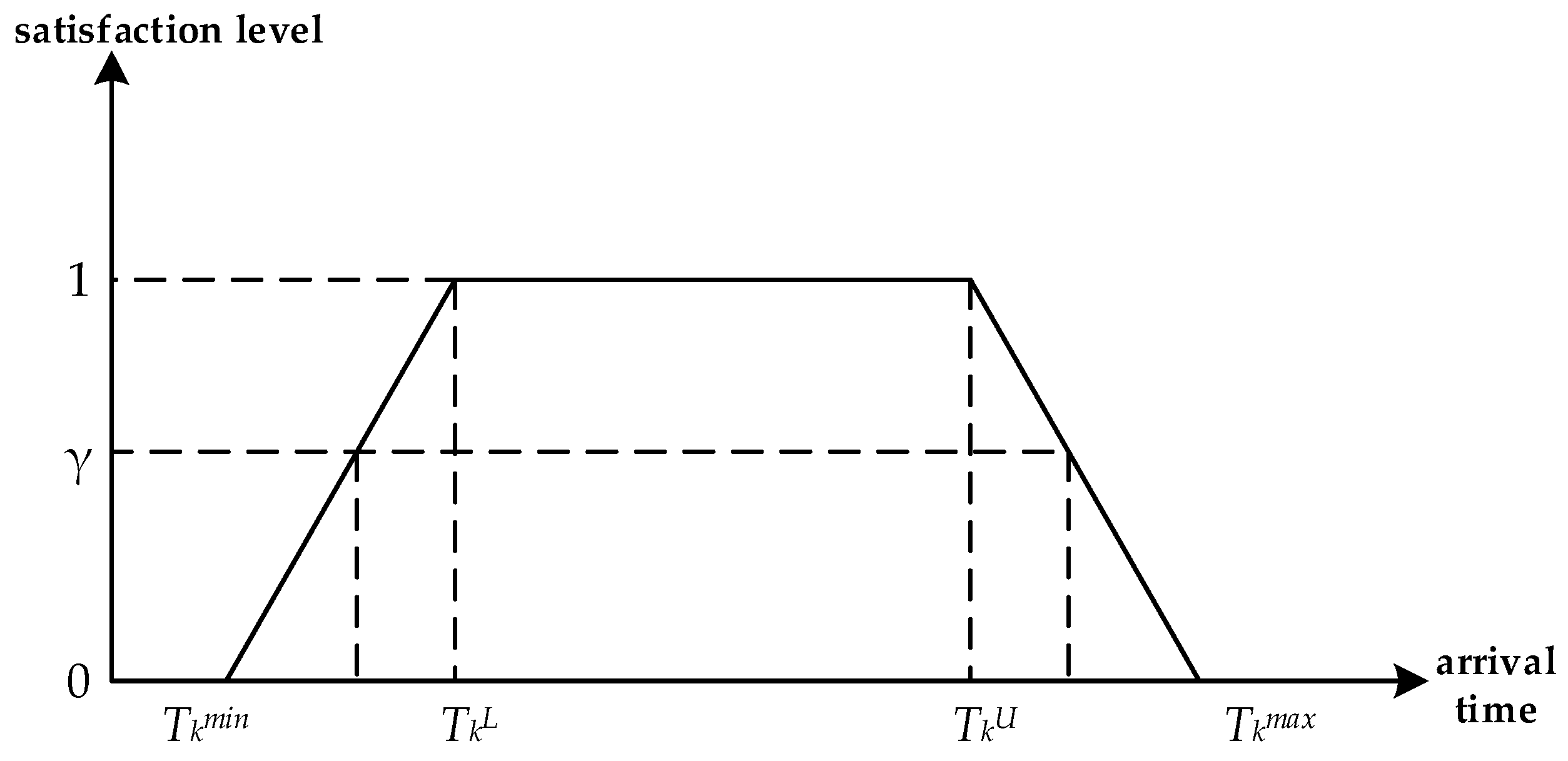
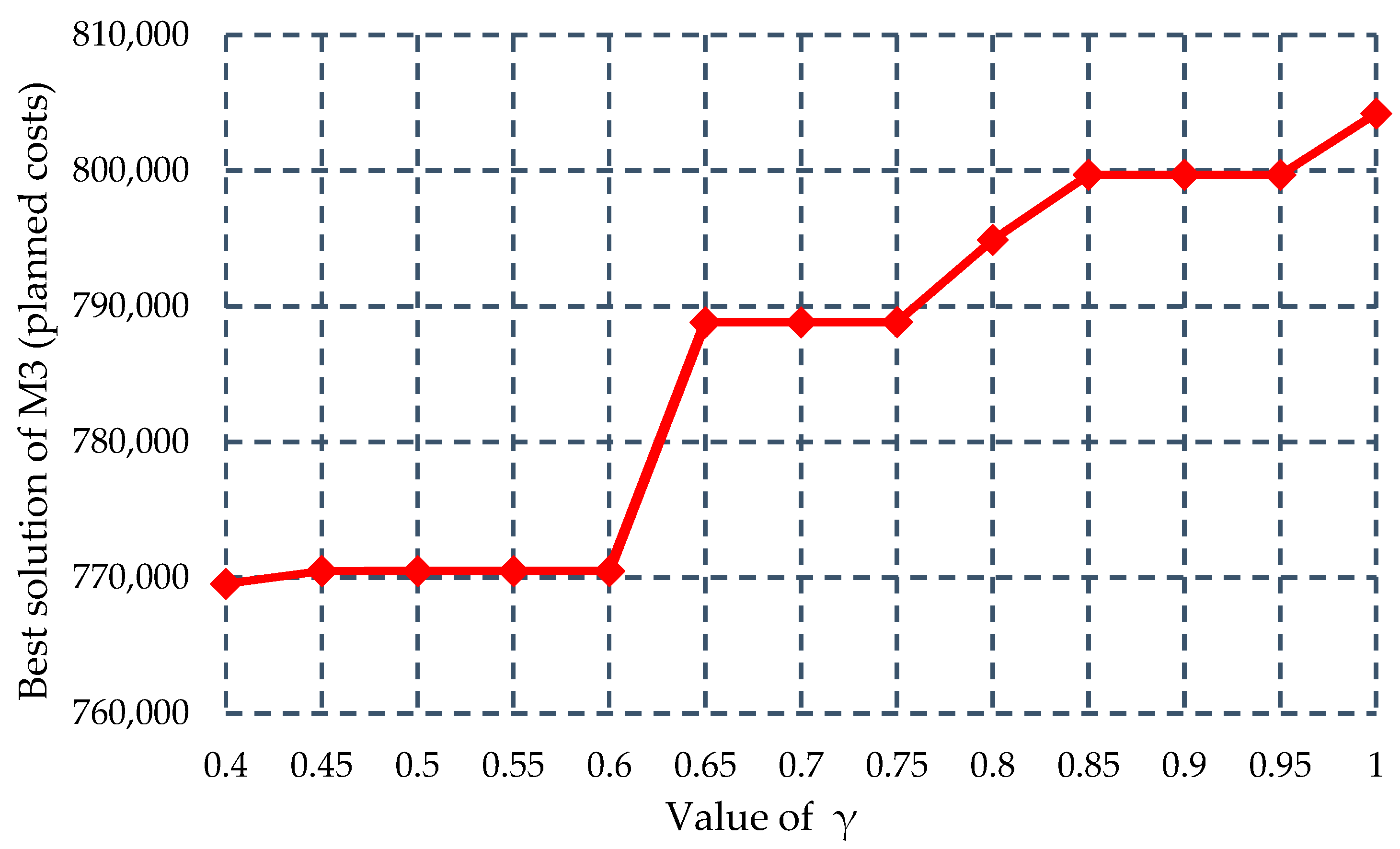
Then, to examine how customer satisfaction level γ influences the multicommodity multimodal routing, we conduct the sensitivity of the best solution of M3 with respect to the value of γ. Let γ vary from 0.4 to 1.0 with step size of 0.05, and keeping α = β = 0.9, we can obtain Figure 6 that illustrates the result of the sensitivity analysis.

As we can see from Figure 6, considering a reasonable customer satisfaction level range, when the customer satisfaction level is lower than 0.6 (γ < 0.6), its variation has only a slight influence on the multicommodity multimodal routing. However, when γ ≥ 0.6, Figure 6 shows that larger values of confidence level γ will result in a larger value of the total generalized costs of the routing, and the increase of the total generalized costs is stepwise. The sensitivity analysis above clearly indicates that restricting the multicommodity multimodal routing to meet stricter customer satisfaction levels will increase the costs of the multimodal service network system to some degree, which is logical according to practical experience.

7. Conclusions

In this study, we apply the fuzzy customer information problem to multicommodity multimodal routing with schedule-based services. The main contribution of this study is that it comprehensively considers the following characteristics in modeling the multimodal routing: (1) multicommodity flows as an optimization object; (2) schedule constraints existing in practice; and (3) fuzzy customer information as the formulation environment. All the formulation characteristics enhance the feasibility of the multimodal routing in dealing with the practical problems. In addition, this study proposes a crisp equivalent method and a linearization method to enable this problem to be formulated by a linear programming model that can be effectively solved by exact solution algorithms (e.g., Branch-and-Bound algorithm). This solving strategy can provide an exact benchmark for systematically testing various heuristic algorithms that will be developed in our future study.

Although several advances have been made by this study, weaknesses still exist. The most significant one is that this study still considers the multimodal service network as a deterministic system. Actually, due to the man–facility–environment impact, operation delays of the container block trains are common, and the travel time of container trucks on the road cannot remain deterministic. Therefore, the multimodal service network is a kind of fuzzy system. Accordingly, our future study will focus on integrating the fuzzy multimodal service network into our current study.

References

1. Sun, Y.; Lang, M. Modeling the Multicommodity Multimodal Routing Problem with Schedule-Based Services and Carbon Dioxide Emission Costs. Math. Probl. Eng. 2015, 2015, 406218. [Google Scholar] [CrossRef]
2. Sun, Y.; Lang, M.; Wang, D. Optimization Models and Solution Algorithms for Freight Routing Planning Problem in the Multi-modal Transportation Networks: A Review of the State-of-the-Art. Open Civ. Eng. J. 2015, 9, 714–723. [Google Scholar] [CrossRef]
3. Janic, M. Modelling the full costs of an intermodal and road freight transport network. Transp. Res. Part D Transp. Environ. 2007, 12, 33–44. [Google Scholar] [CrossRef]
4. Liao, C.H.; Tseng, P.-H.; Lu, C.-S. Comparing carbon dioxide emissions of trucking and intermodal container transport in Taiwan. Transp. Res. Part D Transp. Environ. 2009, 14, 493–496. [Google Scholar] [CrossRef]
5. Zhang, S. Introduction to multimodal transport in America and Canada. Containerization 2009, 20, 6–9. [Google Scholar] [CrossRef]
6. Min, H. International intermodal choices via chance-constrained goal programming. Transp. Res. Part A Gen. 1991, 25, 351–362. [Google Scholar] [CrossRef]
7. Barnhart, C.; Ratliff, H.D. Modeling intermodal routing. J. Bus. Logist. 1993, 14, 205–223. [Google Scholar]
8. Boardman, B.S.; Malstrom, E.M.; Butler, D.P.; Cole, M.H. Computer assisted routing of intermodal shipments. Comput. Ind. Eng. 1997, 33, 311–314. [Google Scholar] [CrossRef]
9. Lozano, A.; Storchi, G. Shortest viable path algorithm in multimodal networks. Transp. Res. Part A Policy Pract. 1997, 35, 225–241. [Google Scholar] [CrossRef]
10. Lam, S.K.; Srikanthan, T. Accelerating the K-Shortest Paths Computation in Multimodal Transportation Networks. In Proceedings of the IEEE 5th International Conference on Intelligent Transportation Systems, Singapore, Singapore, 3–6 September 2002; pp. 491–495.
11. Boussedjra, M.; Bloch, C.; Moudni, A.E.I. An exact method to find the intermodal shortest path (ISP). In Proceedings of the 2004 IEEE International Conference on Networking, Sensing and Control, Taipei, Taiwan, 21–23 March 2004; pp. 1075–1080.
12. Zhang, J.Y.; Guo, Y.H. A multimode transportation network assignment model. J. China Railw. Soc. 2004, 24, 114–116. [Google Scholar]
13. Zhang, Y.H.; Lin, B.L.; Liang, D.; Gao, H.Y. Research on a Generalized Shortest Path Method of Optimizing Intermodal Transportation Problems. J. China Railw. Soc. 2006, 28, 22–26. [Google Scholar]
14. Reddy, V.R.; Kasilingam, R.G. Intermodal transportation considering transfer costs. Available online: http://d.wanfangdata.com.cn/ExternalResource/tdxb201110001%5E1 (accessed on 3 March 2016).
15. Winebrake, J.J.; Corbett, J.J.; Falzarano, A.; Hawker, J.S.; Korfmacher, K.; Ketha, S.; Zilora, S. Assessing energy, environmental, and economic tradeoffs in intermodal freight transportation. J. Air Waste Manag. Assoc. 2008, 58, 1004–1013. [Google Scholar] [CrossRef]
16. Kim, H.J.; Chang, Y.T.; Lee, P.T.W.; Shin, S.H.; Kim, M.J. Optimizing the transportation of international container cargoes in Korea. Marit. Pol. Mgmt. Flagship J. Int. Ship. Port Res. 2008, 35, 103–122. [Google Scholar] [CrossRef]
17. Chang, Y.T.; Lee, P.; Kim, H.J.; Shin, S.H. Optimization model for transportation of container cargoes considering short sea shipping and external cost: South Korean case. Transp. Res. Rec. J. Transp. Res. Board 2010, 2166, 99–108. [Google Scholar] [CrossRef]
18. Liu, J.; He, S.W.; Song, R.; Li, H.D. Study on optimization of dynamic paths of intermodal transportation network based on alternative set of transport modes. J. China Railw. Soc. 2011, 33, 1–6. [Google Scholar]
19. Cho, J.H.; Kim, H.S.; Choi, H.R. An intermodal transport network planning algorithm using dynamic programming-a case study: from Busan to Rotterdam in intermodal freight routing. Appl. Intell. 2012, 36, 529–541. [Google Scholar] [CrossRef]
20. Sun, Y.; Lang, M.X. Bi-objective optimization for multi-modal transportation routing planning problem based on Pareto optimality. J. Ind. Eng. Manag. 2015, 8, 1195–1217. [Google Scholar] [CrossRef]
21. Xiong, G.W.; Wang, Y. Best routes selection in multimodal networks using multi-objective genetic algorithm. J. Combin. Optim. 2014, 28, 655–673. [Google Scholar] [CrossRef]
22. Teodorović, D.; Pavković, G. The fuzzy set theory approach to the vehicle routing problem when demand at nodes is uncertain. Fuzzy Sets Syst. 1996, 82, 307–317. [Google Scholar] [CrossRef]
23. Erbao, C.; Mingyong, L. A hybrid differential evolution algorithm to vehicle routing problem with fuzzy demands. J. Comput. Appl. Math. 2009, 231, 302–310. [Google Scholar] [CrossRef]
24. López-Castro, L.F.; Montoya-Torres, J.R. Vehicle routing with fuzzy time windows using a genetic algorithm. In Proceedings of the 2011 IEEE Workshop on Computational Intelligence in Production And Logistics Systems, Paris, France, 11–15 April 2011; pp. 1–8.
25. Lium, A.G.; Crainic, T.G.; Wallace, S.W. A study of demand stochasticity in service network design. Transp. Sci. 2009, 43, 144–157. [Google Scholar] [CrossRef]
26. Bai, R.; Wallace, S.W.; Li, J.; Chong, A.Y.L. Stochastic service network design with rerouting. Transp. Res. Part B Methodol. 2014, 60, 50–65. [Google Scholar] [CrossRef]
27. Ji, X.; Iwamura, K.; Shao, Z. New models for shortest path problem with fuzzy arc lengths. Appl. Math. Model. 2007, 31, 259–269. [Google Scholar] [CrossRef]
28. Ghannadpour, S.F.; Noori, S.; Tavakkoli-Moghaddam, R.; Ghoseiri, K. A multi-objective dynamic vehicle routing problem with fuzzy time windows: Model, solution and application. Appl. Soft Comput. 2014, 14, 504–527. [Google Scholar] [CrossRef]
29. Liu, B.; Iwamura, K. Chance constrained programming with fuzzy parameters. Fuzzy Sets Syst. 1998, 94, 227–237. [Google Scholar] [CrossRef]
Figure 1. Satisfaction level in the fuzzy soft time window.
Information 07 00013 g001
Figure 2. Diagram of the sufficiency proof.
Information 07 00013 g002
Figure 3. Diagram of the necessity proof.
Information 07 00013 g003
Figure 4. A multimodal service network.
Information 07 00013 g004
Figure 5. Sensitivity of the three kinds of costs with respect to the values of α and β.
Information 07 00013 g005
Figure 6. Sensitivity of the best solution with respect to the value of γ.
Information 07 00013 g006