
The Treewidth of Induced Graphs of Conditional Preference Networks Is Small


Abstract
:
1. Introduction
- 1
- We explore the treewidth problem about the induced graphs of CP-nets— as far as we know, there is no literature availlable to study the treewidth characterization of induced graphs of CP-nets.
- 2
- We design a more efficient algorithm to solve the treewidth of induced graphs of CP-nets utilizing a Bucket Elimination approach; this approach uses the randomness characteristics of input order to speed search.
- 3
- We find that the treewidth of induced graphs of CP-nets is very small; this interesting discovery may lay the foundation for designing an algorithm for solving tractable reasoning tasks, such as dominance queries, in the future.
2. Background on Treewidth and CP-nets
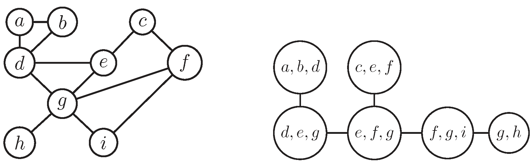
2.1. Treewidth
- (i)
- . That is, each graph vertex is contained in at least one tree node.
- (ii)
- If vertices v and w both are connected in a graph G, then v and w are contained in at least one subset .
- (iii)
- Considering the three nodes in the tree, when j exists in the path of i and k,, that is, common vertices of i and k must appear in the j.

2.2. CP-nets


3. Related Work
4. Treewidth of the Induced Graphs of CP-nets
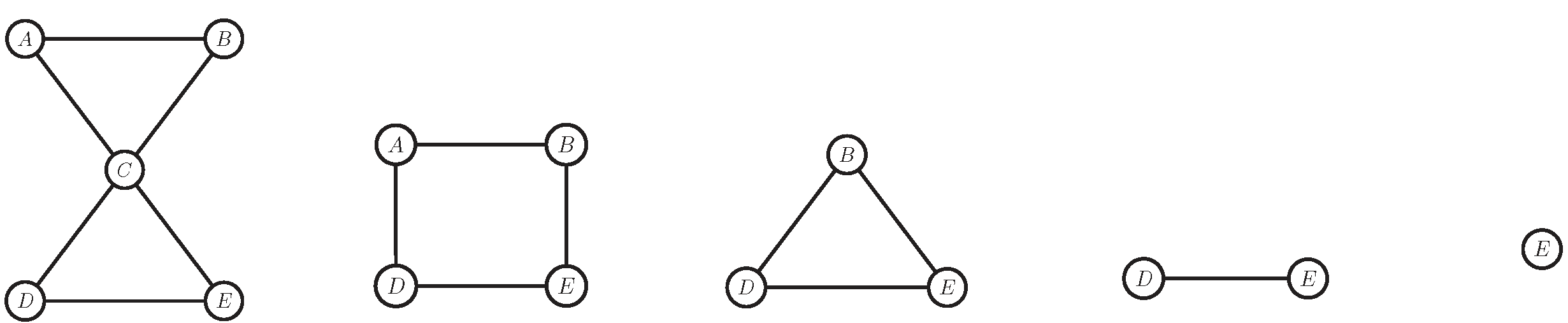
4.1. Bucket Elimination Technique


4.2. Algorithm for the Treewidth of an Induced Graph
| Algorithm 1: solving treewidth of included graphs of CP-nets N′. | |
| Input: An adjacency matrix A[i, j] of induced graph | |
| Output: The treewidth of N′ | |
| 1 | treewidth ← 0; |
| 2 | Mdec ← 0; |
| 3 | mdec ← 0; |
| // Calculate the total number of vertex elimination order sum. | |
 | |
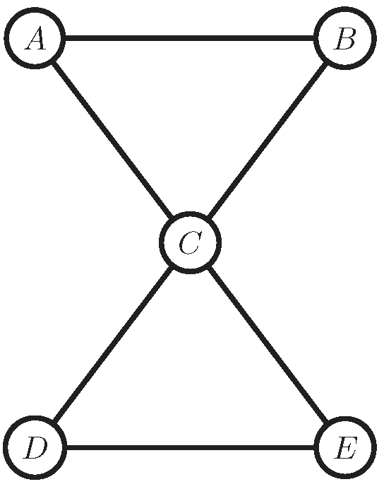
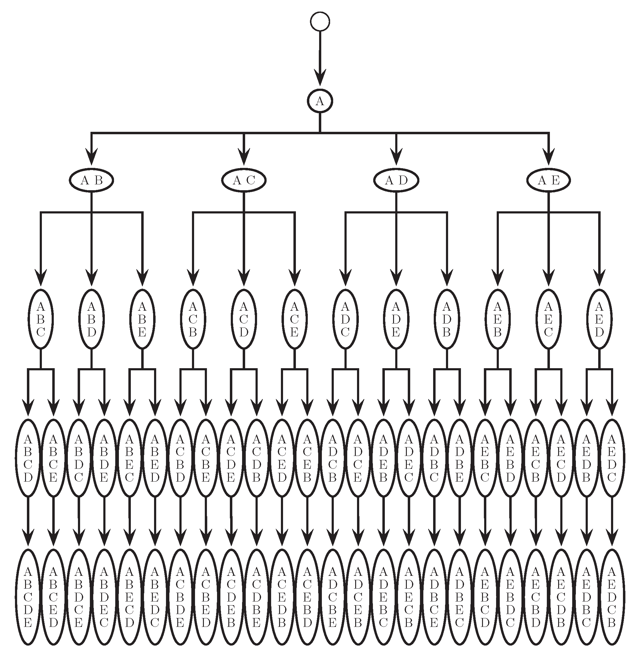
4.3. A Motivate Example

| π | width | |
4.4. Time Complexity Analysis
5. Experimental Evaluation
5.1. Experimental Environment
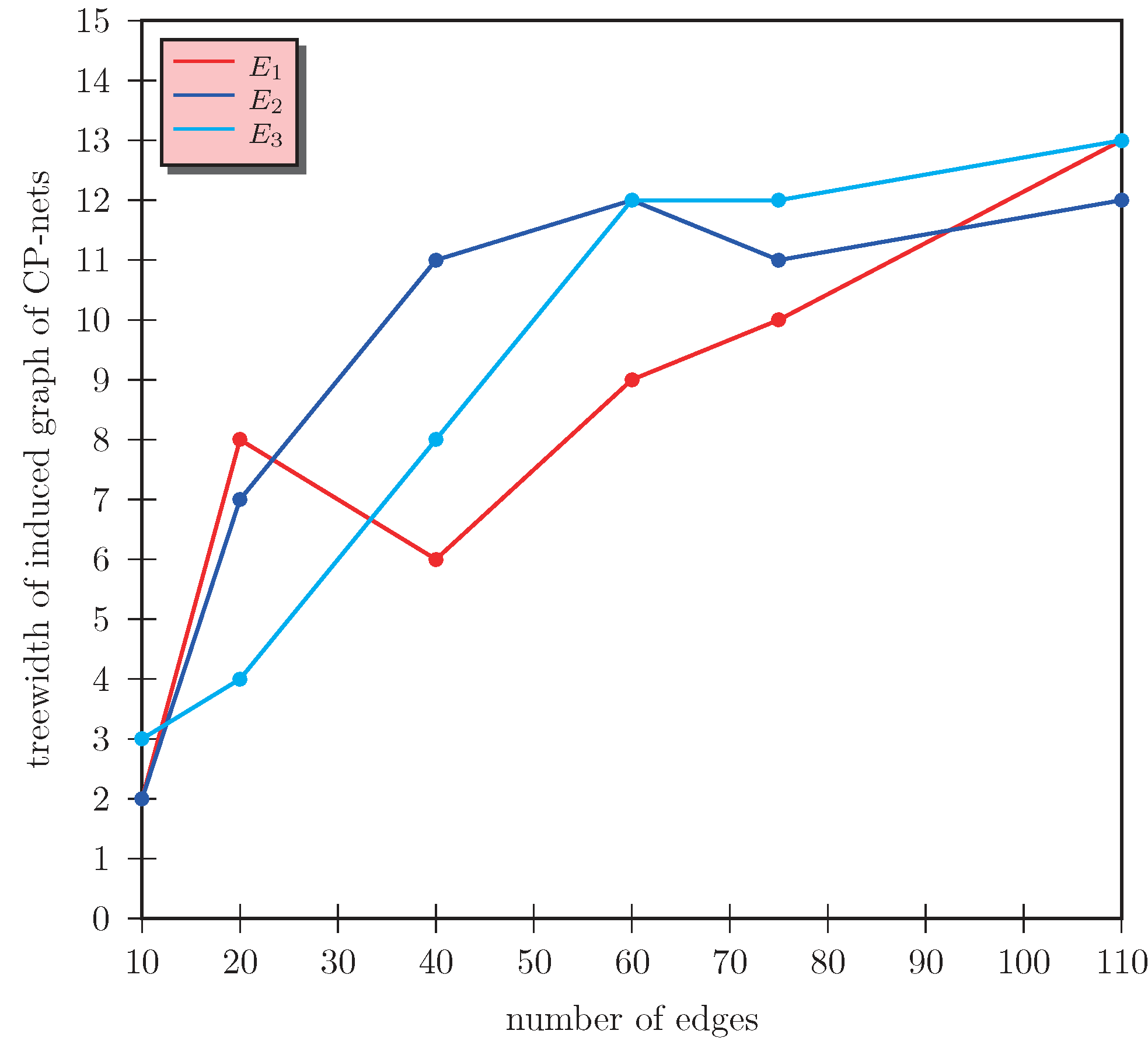
5.2. Experimental Results on Simulated Data
| n | 8 | 16 | 32 | 64 | 128 | 256 | 512 | 1024 |
| |E| | 12 | 32 | 80 | 192 | 448 | 1024 | 2304 | 5120 |
| tw | 1 | 2 | 6 | 7 | 8 | 9 | 9 | 10 |
| time(s) | 0.016 | 0.031 | 0.094 | 0.313 | 1.103 | 4.064 | 15.102 | 61.057 |
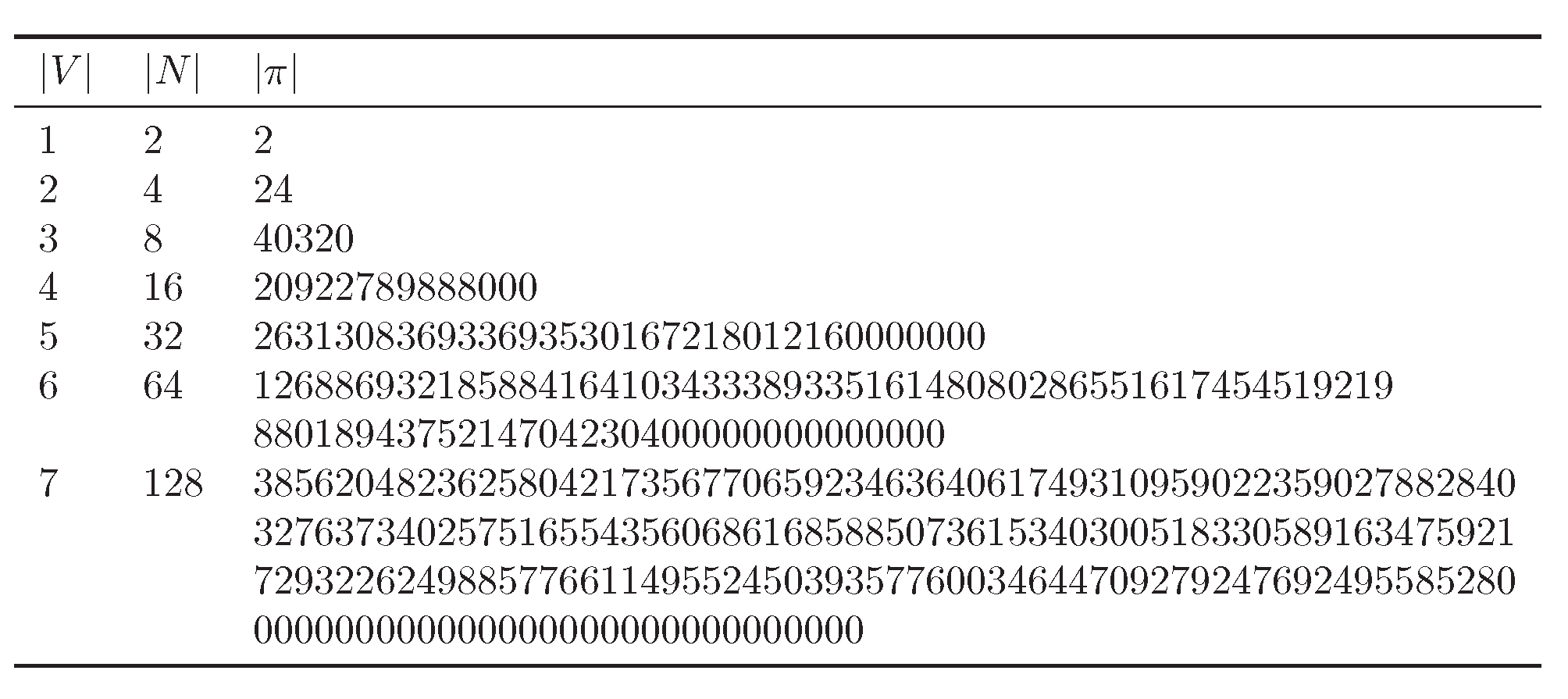
| V | n | ||
|---|---|---|---|
| 2 | 4 | 4 | 6 |
| 3 | 8 | 12 | 28 |
| 4 | 16 | 32 | 128 |
| 5 | 32 | 80 | 496 |
| 6 | 64 | 192 | 2016 |
| 7 | 128 | 448 | 8128 |

6. Conclusions and Future Work
Acknowledgments
Author Contributions
Conflicts of Interest
References
- Boutilier, C.; Brafman, R.; Domshlak, C.; Hoos, H.; Poole, D. CP-nets: A tool for representing and reasoning with conditional ceteris paribus preference statements. J. Artif. Intell. Res. 2004, 21, 135–191. [Google Scholar]
- Liu, J.L.; Liao, S.Z. Expressive efficiency of two kinds of specific CP-nets. Inf. Sci. 2015, 295, 379–394. [Google Scholar] [CrossRef]
- Majid, Z.A.L.; Emrouznejad, A.; Mustafa, A.; Al-Eraqi, A.S. Aggregating preference ranking with fuzzy Data Envelopment Analysis. Knowl. Based Syst. 2010, 23, 512–519. [Google Scholar]
- Chen, H.; Zhou, L.; Han, B. On compatibility of uncertain additive linguistic preference relations and its application in the group decision making. Knowl. Based Syst. 2011, 24, 816–823. [Google Scholar] [CrossRef]
- Ha, V.; Haddawy, P. Toward Case-Based Preference Elicitation: Similarity Measures on Preference Structures. In Proceedings of the 14th Conference on Uncertainty in Artificial Intelligence, Madison, WI, USA, 24–26 July 1998; pp. 193–201.
- Mindolin, D.; Chomicki, J. Contracting preference relations for database applications. Artif. Intell. 2009, 175, 1092–1121. [Google Scholar] [CrossRef]
- Garey, M.R.; Johnson, D.S. Computers and Intractability: A Guide to the Theory of NP-Completeness; W.H. Freeman: San Francisco, CA, USA, 1979. [Google Scholar]
- Downey, R.G.; Fellows, M.R. Parameterized Complexity; Springer: Berlin/Heidelberg, Germany, 2012. [Google Scholar]
- Chen, J.E. Parameterized computation and complexity: A new approach dealing with NP-hardness. J. Comput. Sci. Technol. 2005, 20, 18–37. [Google Scholar] [CrossRef]
- Robertson, N.; Seymour, P.D. Graph minors. II. Algorithmic aspects of tree-width. J. Algorithms 1986, 7, 309–322. [Google Scholar] [CrossRef]
- Mattei, N.; Pini, M.S.; Rossi, F.; Venable, K.B. Bribery in voting with CP-nets. Ann. Math. Artif. Intell. 2013, 68, 135–160. [Google Scholar] [CrossRef]
- Dechter, R. Bucket elimination: A unifying framework for probabilistic inference. In Learning in Graphical Models; Springer: Berlin/Heidelberg, Germany, 1998; pp. 75–104. [Google Scholar]
- Darwiche, A. Modeling and Reasoning With Bayesian Networks; Cambridge University Press: Cambridge, UK, 2009. [Google Scholar]
- Kosowski, A.; Li, B.; Nisse, N.; Suchan, K. k-chordal graphs: From cops and robber to compact routing via treewidth. In Automata, Languages, and Programming; Springer: Berlin/Heidelberg, Germany, 2012; pp. 610–622. [Google Scholar]
- Dow, P.A. Search Algorithms for Exact Treewidth. Ph.D. Thesis, University of California Los Angeles, Los Angeles, CA, USA, 2010. [Google Scholar]
- Gao, W.Y.; Li, S.H. Tree decomposition and its Application in Algorithm: Survey. Comput. Sci. 2012, 39, 14–18. [Google Scholar]
- Arnborg, S.; Corneil, D.G.; Proskurowski, A. Complexity of finding embeddings in ak-tree. SIAM J. Algebraic Discret. Methods 1987, 8, 277–284. [Google Scholar] [CrossRef]
- Bodlaender, H.L.; Fomin, F.V.; Koster, A.M.; Kratsch, D.; Thilikos, D.M. On Exact Algorithms for Treewidth; Springer: Berlin/Heidelberg, Germany, 2006. [Google Scholar]
- Kießling, W. Foundations of preferences in database systems. In Proceedings of the 28th International Conference on Very Large Data Bases, Hong Kong, China, 20–23 August 2002; pp. 311–322.
- Guerin, J.T.; Allen, T.E.; Goldsmith, J. Learning CP-net Preferences online from user queries. In Algorithmic Decision Theory; Springer: Berlin/Heidelberg, Germany, 2013; pp. 208–220. [Google Scholar]
- Bigot, D.; Mengin, J.; Zanuttini, B. Learning probabilistic CP-nets from observations of optimal items. In Proceedings of the 7th European Starting AI Researcher Symposium, Prague, Czech Republic, 18–19 August 2014; IOS Press: Amsterdam, The Netherlands, 2014; pp. 81–90. [Google Scholar]
- Liu, W.Y.; Wu, C.H.; Feng, B.; Liu, J.T. Conditional preference in recommender systems. Expert Syst. Appl. 2015, 42, 774–788. [Google Scholar] [CrossRef]
- Goldsmith, J.; Lang, J.; Truszczynski, M.; Wilson, N. The computational complexity of dominance and consistency in CP-nets. J. Artif. Intell. Res. 2008, 33, 403–432. [Google Scholar]
- Bodlaender, H.L.; Thilikos, D.M. Treewidth for graphs with small chordality. Discret. Appl. Math. 1997, 79, 45–61. [Google Scholar] [CrossRef]
- Bodlaender, H.L. A linear time algorithm for finding tree-decompositions of small treewidth. In Proceedings of the 25th Annual ACM Symposium on Theory of Computing, San Diego, CA, USA, 16–18 May 1993; ACM: New York, NY, USA, 1993; pp. 226–234. [Google Scholar]
- Dinneen, M.J.; Khosravani, M. A linear time algorithm for the minimum spanning caterpillar problem for bounded treewidth graphs. In Structural Information and Communication Complexity; Springer: Berlin/Heidelberg, Germany, 2010; pp. 237–246. [Google Scholar]
- Bodlaender, H.L.; Möhring, R.H. The pathwidth and treewidth of cographs. SIAM J. Discret. Math. 1993, 6, 181–188. [Google Scholar] [CrossRef]
- Sundaram, R.; Singh, K.S.; Rangan, C.P. Treewidth of circular-arc graphs. SIAM J. Discret. Math. 1994, 7, 647–655. [Google Scholar] [CrossRef]
- Kloks, T.; Kratsch, D. Treewidth of chordal bipartite graphs. J. Algorithms 1995, 19, 266–281. [Google Scholar] [CrossRef]
- Koster, A.M.; van Hoesel, S.P.; Kolen, A.W. Solving partial constraint satisfaction problems with tree decomposition. Networks 2002, 40, 170–180. [Google Scholar] [CrossRef]
- Zhao, J.; Che, D.; Cai, L. Comparative pathway annotation with protein-DNA interaction and operon information via graph tree decomposition. Pac. Symp. Biocomput. 2007, 12, 496–507. [Google Scholar]
- Zhao, J.; Malmberg, R.L.; Cai, L. Rapid ab initio prediction of RNA pseudoknots via graph tree decomposition. J. Math. Biol. 2008, 56, 145–159. [Google Scholar] [CrossRef] [PubMed]
- De Givry, S.; Schiex, T.; Verfaillie, G. Exploiting tree decomposition and soft local consistency in weighted CSP. In Proceedings of the 21st National Conference on Artificial Intelligence, Boston, MA, USA, 16–20 July 2006; Volume 6, pp. 1–6.
- Jégou, P.; Ndiaye, S.; Terrioux, C. Dynamic Heuristics for Backtrack Search on Tree-Decomposition of CSPs. In Proceedings of the 20th International Joint Conference on Artificial Intelligence, Hyderabad, India, 6–12 January 2007; pp. 112–117.
- Planken, L.; de Weerdt, M.; van der Krogt, R. Computing All-Pairs Shortest Paths by Leveraging Low Treewidth. J. Artif. Intell. Res. 2012, 43, 353–388. [Google Scholar]
- Bertele, U.; Brioschi, F. Nonserial Dynamic Programming; Elsevier: Amsterdam, The Netherlands, 1972. [Google Scholar]
- Zhang, C.; Naughton, J.; DeWitt, D.; Luo, Q.; Lohman, G. On supporting containment queries in relational database management systems. In Proceedings of the 2001 ACM SIGMOD International Conference on Management of Data, Santa Barbara, CA, USA, 21–24 May 2001; Volume 30, pp. 425–436.
- Shoikhet, K.; Geiger, D. A practical algorithm for finding optimal triangulations. In Proceedings of the Fourteenth National Conference on Artificial Intelligence and Ninth Innovative Applications of Artificial Intelligence Conference, Providence, RI, USA, 27–31 July 1997; pp. 185–190.
© 2016 by the authors; licensee MDPI, Basel, Switzerland. This article is an open access article distributed under the terms and conditions of the Creative Commons by Attribution (CC-BY) license (http://creativecommons.org/licenses/by/4.0/).
Share and Cite
Liu, J.; Liu, J. The Treewidth of Induced Graphs of Conditional Preference Networks Is Small. Information 2016, 7, 5. https://doi.org/10.3390/info7010005
Liu J, Liu J. The Treewidth of Induced Graphs of Conditional Preference Networks Is Small. Information. 2016; 7(1):5. https://doi.org/10.3390/info7010005
Chicago/Turabian StyleLiu, Jie, and Jinglei Liu. 2016. "The Treewidth of Induced Graphs of Conditional Preference Networks Is Small" Information 7, no. 1: 5. https://doi.org/10.3390/info7010005
APA StyleLiu, J., & Liu, J. (2016). The Treewidth of Induced Graphs of Conditional Preference Networks Is Small. Information, 7(1), 5. https://doi.org/10.3390/info7010005