Article

An Image Compression Scheme in Wireless Multimedia Sensor Networks Based on NMF

1
School of Computer, Nanjing University of Posts and Telecommunications, Nanjing 210003, China
2
Jiangsu High Technology Research Key Laboratory for Wireless Sensor Networks, Nanjing University of Posts and Telecommunications, Nanjing 210003, China
3
Key Laboratory of Broadband Wireless Communication and Sensor Network Technology, Ministry of Education, Nanjing 210003, China
*
Author to whom correspondence should be addressed.
Information 2017, 8(1), 26; https://doi.org/10.3390/info8010026
Submission received: 14 December 2016 / Accepted: 7 February 2017 / Published: 24 February 2017

Abstract

:
With the goal of addressing the issue of image compression in wireless multimedia sensor networks with high recovered quality and low energy consumption, an image compression and transmission scheme based on non-negative matrix factorization (NMF) is proposed in this paper. First, the NMF algorithm theory is studied. Then, a collaborative mechanism of image capture, block, compression and transmission is completed. Camera nodes capture images and send them to ordinary nodes which use an NMF algorithm for image compression. Compressed images are transmitted to the station by the cluster head node and received from ordinary nodes. The station takes on the image restoration. Simulation results show that, compared with the JPEG2000 and singular value decomposition (SVD) compression schemes, the proposed scheme has a higher quality of recovered images and lower total node energy consumption. It is beneficial to reduce the burden of energy consumption and prolong the life of the whole network system, which has great significance for practical applications of WMSNs.

1. Introduction

Wireless multimedia sensor networks (WMSNs) are a new type of distributed sensing network. They mainly consist of a set of multimedia sensor nodes capable of computing, storing and communicating [1]. WMSNs can perceive a variety of media information from the surrounding environment which are sensed by multimedia sensor nodes, including images, video, numerical, audio and other information.
WMSNs is a specific development of traditional wireless sensor networks (WSNs) for this application. It has some unique characteristics [2] such as the following:
  • Energy consumption and resource requirements: The key issue in WSNs is energy consumption, as recognized by research scholars. The process of wireless transmission and reception consumes the largest part of the energy in traditional WSNs. However, sensors in most WSNs are typically battery-powered, and batteries are usually infeasible in terms of being recharged or even replaced [3]. In WMSNs, sensor nodes will collect much other video and image data and consume large amounts of energy. Meanwhile, compared to conventional WSNs, since the collected audio and image information constitute a large amount of data, the bandwidth required for transmission is wider.
  • Local processing: WMSNs can be employed in the local image processing methods to reduce the amount of data among networks, such as simple image processing algorithms for background extraction from moving targets, or complex algorithms for feature extraction or scenario inference. Which algorithm to use and what level of complexity required is determined by physical conditions. For example, if you want to get information from the environment, we can use the low-level difference algorithm for edge detection [4]. If you also need a higher-level image processing mode, then we can apply complex algorithms to classify the collected targets in a basic manner.
WMSNs is a seriously resource-constrained network mechanism. Under such conditions, the entire network performance will be greatly influenced if we spend too much energy on image acquisition and processing, especially for a high degree of repeated data. In most cases, only one or two nodes wake up to monitor the implementation of image collection when an event occurs in view of the above limitations. At this time, the strategy adopted to reduce energy consumption mainly includes compression and transmission of the captured image.
As can be seen from the existing work, efficient image compression is needed to reduce the energy consumption of individual nodes and extend the life of the network in WMSNs. However, implementation of previous deep exploration in image compression lasted a long time. JPEG and JPEG2000 coding is widely used in transmissions in WMSNs [5]. The singular value decomposition (SVD) adaptive image compression method has been raised in a recent study [6]. These methods solve the collaborative problem of image compression in WMSNs to some degree, but they still have their own advantages and disadvantages. Especially in terms of energy consumption, the JPEG2000 method has a distinct weakness due to topology design. On the other hand, the SVD method exhibits many side effects in recovered images, which would have an impact on image quality.
Considering this, an image compression and transmission scheme based on non-negative matrix factorization (NMF) is proposed in this paper. We improve the existing non-negative matrix factorization algorithm and propose a multilayer NMF framework. While taking advantage of node cooperation, a characteristic of WMSNs, compression tasks are decomposed efficiently. It can make full use of the resources of each ordinary node and maintain a more balanced energy state to avoid instant incapacitation in the network, so that we can reduce energy consumption and extend the life cycle of the network, while partly reducing the noise of the image. This is vital to extending the lifetime of the whole network, which means a great deal when the network is being used for purposes such as military surveillance or industrial supervision. We can also effectively eliminate the block edge effect and improve the quality of the restored image. Therefore, the application fields for this scheme could be expanded to include video monitoring in various scenarios.

2. NMF Method and Network Model

2.1. NMF Method

In 1999, an article published in Nature proposed the NMF (Non-negative Matrix Factorization) algorithm, with the following functions [7]: factorize a non-negative matrix product of two new low-rank non-negative matrices, and only additive combinations are allowed to appear [8]. The published papers quickly attracted the attention of researchers in many fields, and provoked a great deal of further study [9].
In 2003, the non-negative matrix factorization has been interpreted geometrically and analyzed with synthetic image database under certain conditions [10]. The separability assumption turns NMF into a tractable problem. Also, a highly scalable and empirically noise robust NMF algorithm was derived in recent years [11] which shows the special significance of the NMF method.
Assume a non-negative data set { x 1 , x 2 , ... , x n } , the following formula can express the NMF algorithm:
x i j = 1 r c j i b j , i = 1 , 2 , ... , n
wherein x i + m × 1 , b i + m × 1 is the base vector, c j i 0 for the coefficients. r < < min ( m , n ) is a common condition for the selection of the base. So, the compression efficiency of the original data set (e.g., image) can be increased.
X = ( x 1 , x 2 , ... , x n ) , B = ( b 1 , b 2 , ... , b r ) , C = ( c j i ) r × n . Equation (1) is equivalent to
X B C
The minimization problem shown below aims to solve the best non-negative low rank of approximation of matrix X:
min D ( X , B C ) s . t . B 0 , C 0
D(X, BC) here represents cost function, which also known as “distance”, to measure X and BC. There are a variety of common cost functions as following:
  • Euclidean distance:
    D ( X , B C ) = X B C F 2
    Euclidean distance is more suitable for channels with Gaussian noise.
  • General Kullback-Leibler distance:
    D ( X , B C ) = i j ( x i j log x i j ( B C ) i j x i j + ( B C ) i j )
    General Kullback-Leibler distance is more suitable for channels with Additive Poisson noise.
  • Bregman distance:
    D ( X , B C ) = i j ( ( φ ( x i j ) φ ( ( B C ) i j ) ) φ ( ( B C ) i j ) ( x i j ( B C ) i j ) )
    Especially, if φ ( x ) = x 2 / 2 , Bregman distance is equivalent to Euclidean distance. If φ ( x ) = x log x x , Bregman distance is equivalent to General Kullback-Leibler distance.
  • Csiszár distance:
    D ( X , B C ) = i j ( B C ) i j φ ( x i j ( B C ) i j )
Euclidean distance [12] is the most frequently function used as the Formula (4). Such function is suitable for additive Gaussian noise conditions. In this case, the optimization problem in Equation (3) is re-described as
min X B C F 2 s . t . B 0 , C 0
There are many methods for solving optimization problems such as Formula (8). From a mathematical perspective, Formula (8) is convex with regard to both B and C which can be well utilized. There are three common methods: Adaptive Non-Linear Sampling (ANLS) method [13], the Projection Gradient method and the Multiplicative Update method. From a common point of view, we choose an alternating method to solve the Non-Negative Least Squares algorithm called Adaptive Non-Linear Sampling (ANLS). The ANLS runs as following Algorithm 1 below.
In the ANLS algorithm, there are some limitations that make this algorithm consume more time in execution. For instance, we have to determine the number of the executions alternating operation (i.e., step) when doing non-negative least squares correlation calculation.
The NMF algorithm can provide a valid constraint and sometimes “correct” results [14]. Also, the image can be considered as a matrix. At the same time, the process of rebuilding is similar to a combination of localities which has a specific physical meaning [15]. Considering these aspects, we chose the NMF algorithm to do the compression of images in WMSNs.
Algorithm 1. Adaptive Non-Linear Sampling Algorithm.
1: Initialize 2 non-negative matrices B, C;
2: First, set matrix C as a constant value, solve the Non-Negative Least Squares Problem with matrix B. Record the calculating times used above as m so matrix B consists of m optimal solutions ultimately.
3: Then, set matrix B as a constant value similarly, solve the Non-Negative Least Squares Problem with matrix C. Record the calculating times used above as n so matrix C consists of n optimal solutions ultimately.
4: If matrix B, C meet the requirements of stopping Least Square algorithm, then finish the calculation. Else, turn to Step 2.

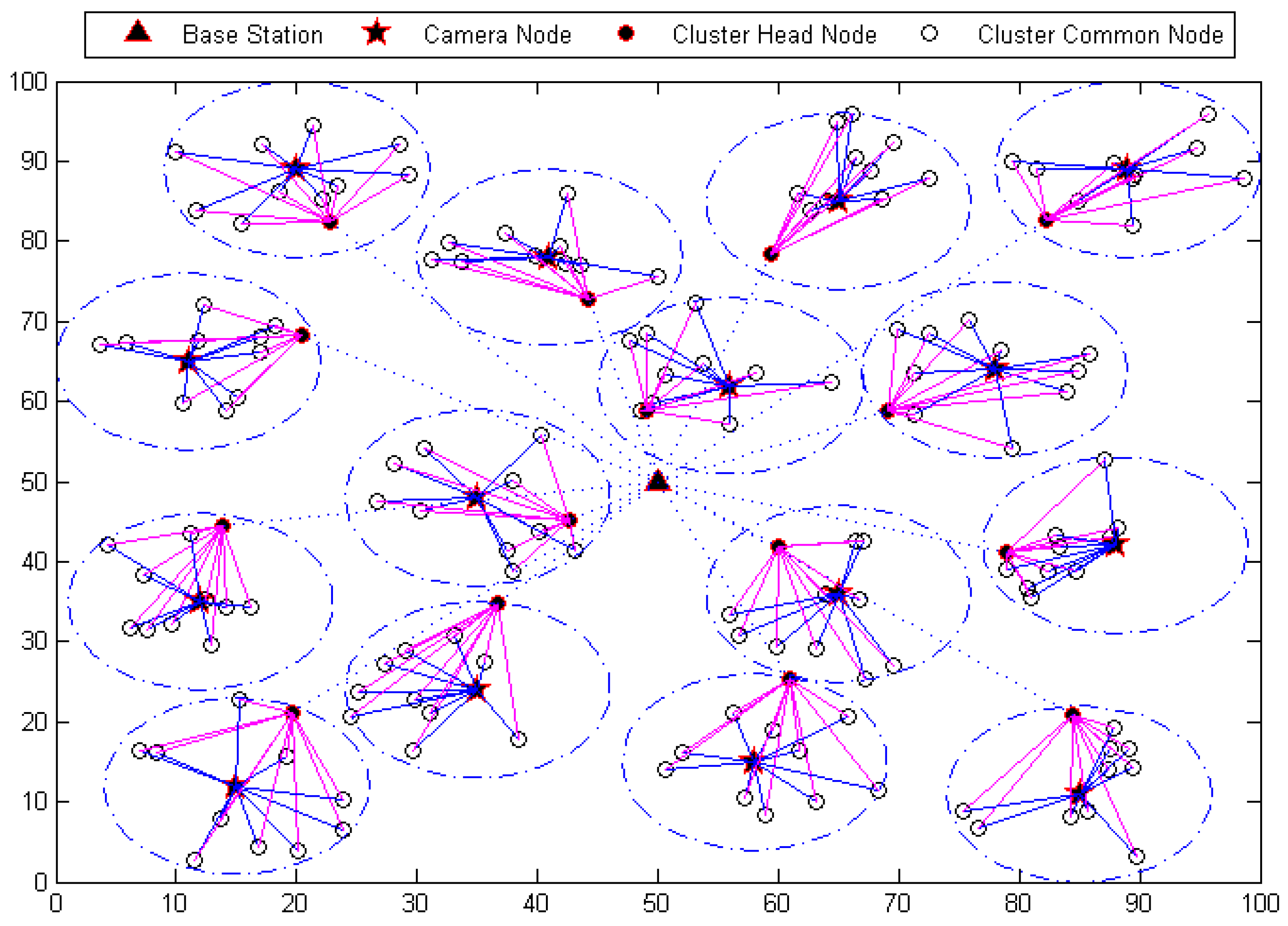
2.2. Network Topology Structure

One of the core points to improve WMSNs performance is to do our best to make the lifetime of the network as long as possible and to ensure that the image capture and transfer are regular at the same time. Based on this, we selected the layer-cluster topology. This model can decompose images more efficiently.
First, the network nodes are divided into image acquisition nodes (also known as camera nodes) and ordinary nodes with the assumptions below:
  • Node ID numbers are not allowed to be duplicated in the network, and each node has a unique identity. All nodes must ensure time synchronization after being deployed;
  • The camera nodes are deployed fixedly and different camera nodes must monitor different areas which have no duplicate parts, i.e., the distance between two cameras must be at least two nodes radius and a wireless communication connection;
  • The ordinary nodes are deployed randomly around the camera nodes with large density in order to make sure that the camera nodes can be connected to the neighboring ordinary nodes in a communication range.
Building a topology for inter-node cooperation and construction of compressing transmission based on these assumptions is a very critical process. The topology structure is constructed in the following steps:
  • The camera nodes are placed in the center of the monitoring range. Then, each ordinary node which could be connected is structured to a cluster;
  • A cluster head node should be selected in the cluster composed. Requirements are: to establish the best quality route to communicate with the base station, and to ensure adequate energy reserve. Assuming that the initial energy reserves of all nodes are basically the same, the node which is nearest to the base station is usually selected as the cluster head node;
  • The cluster head nodes use broadcast channels to inform their ID numbers and camera node ID numbers to ordinary nodes within the cluster;
  • Each ordinary node then sends their ID numbers to the camera nodes and cluster head nodes;
  • The cluster head nodes and camera nodes record all ID numbers received.
The steps above are the construction method of a collaborating image compression-transmission network topology. The expected purpose is to form a calculating cluster structure based on the existence of ordinary nodes which are in the communication range of camera nodes. The process of establishing this structure occupies a very prominent position in the compression algorithm mechanisms.

2.3. Network Energy Consumption Model

As they are irreplaceable, battery-operated devices, sensors in WMSNs usually consume even more energy than in WSNs [16]. The Heizelman model is one of the communication energy models most commonly used by researchers [17]. In this paper, we also used this model to design simulation experiments. Energy consumption of communication is composed by a transmitting unit and a receiving unit. The energy consumption of the transmitting unit is expressed by E S ( J , d ) , while the energy of the receiving unit is expressed by E R ( J ) × B . The transmission and reception circuit energy consumption is indicated with E e l e c . There are two signal fading concepts as the decline of free space d 2 , namely slow fading, and multipath effects d 4 , namely fast fading. The function of the signal amplifier is to provide subsequent energy to the signal, μ f s is a parameter of d 2 , μ a m p is a parameter of d 4 . The distance threshold set for the sending and receiving ends is d 0 , usually assumed as the communication radius. If the radius is less than d 0 , it takes a slow fading mode (fs). Otherwise it takes the fast fading mode (mp). Signal fading is originated from distance between transmit-receive ends.
Suppose a node transmitting a package in a time slot, the transmission distance of the package is d and the package size is assumed to be 1 bit. Then, the sensor launches unit energy consumption at this time according to the following formula:
E s ( J , d ) = { E e l e c + μ f s d 2 , d < d 0 E e l e c + μ u m p d 4 , d d 0
The receiving unit receives 1 bit data consumed energy as follows:
E R ( J ) = E e l e c
Network total energy consumptions consist of communication energy consumption, collecting energy consumption and image compression energy consumption. A single-hop communicating policy is adopted between the camera nodes and the ordinary nodes in the network. The ordinary nodes and the head nodes use the same method.
Assuming k as the total number of the ordinary nodes and the camera nodes, these k nodes should be located within the communication range of the camera nodes. Suppose the size of the image camera node captured is m × n, the size of an image block is p × q. The distance between a head node and each ordinary node is d 1 , d 2 , L , d k . The distance between the base station and a cluster head node is d c h s . Assuming the distance between a camera and an ordinary node as l 1 , l 2 , L , l k , in terms of simplicity, we suppose all ordinary nodes have the same amount of initial energy reserved and assuming the same probability η . This refers to the probability of the camera node transmitting information to all ordinary nodes.
η = m × n p × q k
η > 1 when the original image is divided into a plurality of blocks, and the number of blocks is even more than the total number of the ordinary nodes.
Assume that a camera node sends c bits of data to an ordinary node in a process of transmission and the image capture energy consumption of the camera node is represented by W. Then the energy consumption of the camera in each cluster is shown in Equation (12):
E c d = W + η ( c E e l e c + c μ f s l 1 2 ) + η ( c E e l e c + c μ f s l 2 2 ) + η ( c E e l e c + c μ f s l k 2 ) = W + η c i = 1 k ( E e l e c + μ f s l i 2 ) = W + η c ( k E e l e c + i = 1 k μ f s l i 2 )
Energy consumption of each ordinary node can be split into three parts, including sending data, receiving data and the compression work part. Suppose that we want to get the lowest image quality after compressing and restoring with the algorithm, then set compression ratio as ρ i , energy consumption of compressing per bit data as E c p . The energy consumption of an ordinary node can be expressed as follows:
E c d = η c E e l e c + η c E c p + n c ρ i ( E e l e c + μ f s d i 2 ) = η c ( E e l e c + ( 1 + 1 ρ i ) E e l e c + 1 ρ i μ f s d i 2 )
The energy consumption of a head node consists of two parts. The total energy consumption is calculated in Formula (14).
E c h = { k η c ρ E e l e c + k η c ρ E e l e c + k η c ρ μ f s d c h s 2 ,      d c h s < d 0 k η c ρ E e l e c + k η c ρ E e l e c + k η c ρ μ u m p d c h s 4 ,      d c h s d 0 = { k η c ρ ( 2 E e l e c + μ f s d c h s 2 ) ,          d c h s < d 0 k η c ρ ( 2 E e l e c + μ u m p d c h s 4 ) ,      d c h s d 0
ρ above refers to the real compression ratio after the base station doing data recovery.
In this paper, we focused on the energy consumption referring to the compressing process and transmission. Processing data refers to the use of the NMF algorithm compression and restoration work, including the energy model selected [18] below using Formula (15).
E = N C V d d 2
where N is the completion of a task occupied period, V d d represents the processor voltage and C is set as 0.67 nF capacitors. This is a complete cycle transition. The Heizelman model has been proved to be adaptable to the large-scale networks [19] so that we chose it to do the simulation.

3. Adaptive Blocking Image Compression Mechanism Based on the NMF Method

3.1. Adaptive Blocking Image Compression Algorithm Based on the NMF

When processing origin images, the NMF algorithm needs to execute more iteration times to get a better image quality. This results in large amounts of computation. We can divide origin images into several blocks and take the adaptive image compression algorithm based on the NMF to process each image block. Experiments show that when each block matrix is small, we can get a higher compression ratio and a higher quality of image restoration by using the NMF method with a few iterations.
The compression ratio of the NMF method only depends on the size of the rank of the base matrix. Therefore, compression ratio can be adaptively adjusted to the energy consumption demands. When a node’s energy depleted, we can choose a lower quality to improve the compression ratio in order to save energy. Suppose an original image with size of m × n , is divided into several blocks the sizes of which are p × q . The image compression ratio obtained after restoration is as Formula (16) shows below.
ρ = i = 1 m * n p * q p * q p * r i + r i * q m * n p * q = i = 1 m * n p * q p * q r i ( p + q ) m * n p * q = i = 1 m * n p * q ( p * q ) 2 r i ( p + q ) m * n
The adaptive blocking image compression method based on the NMF is shown in Algorithm 2.
Figure 1 shows that we can do a simulation experiment by taking the block method based on the SVD and the NMF in this paper respectively on a 512 × 512 × 8 bit Lena image. Results show that the NMF method has a considerable advantage when the compression ratio is consistent with the SVD method. While noting that the more blocks and the smaller the size of the images, the more artifacts and edge effects the SVD method has. This results in lower image restoration quality, which can be seen from the P (Peak Signal to Noise Ratio, PSNR) with S (Size), B (Block number) and R (Compression ratio) data.
Algorithm 2. Adaptive blocking image compression method based on the NMF.
1: V = Block (Origin Figure); // V is a divided piece from original image;
2: Set rank r of decomposition matrix;
3: Set initial value of W = V (:, 1: r), H = V (1: r, :); // initial base W, factor H;
4: Iteration:
W i a W i a μ V i μ ( W H ) i μ H a μ W i a W i a j W j a H a μ H a μ i V i μ ( W H ) i μ
5: If d = V W H F 2 < τ , or the execution time T exceeds the limit value ε , the iteration is terminated. Otherwise, go to Step 4;
6: Restoration of image matrices after compression:
V = ( W H ) i μ = a = 1 r W i a H a μ
Moreover, we undertake a simulation experiment between the NMF method and the SPIHT method. The SPIHT algorithm is a fast and effective technique for image compression. It is spatial tree-based and exploits magnitude correlation across bands of the decomposition [20]. Also, the SPIHT method possesses a lower computational complexity than the NMF method. Based on the above points, the SPIHT method has been selected for the contrast experiment.
We choose three different image block numbers for the NMF method. Figure 2 shows that, when NMF and SPIHT share the same compression ratio (e.g., 0.25 bpp), the NMF method has a slight disadvantage to SPIHT but shows a considerable advantage when the block number increases constantly. The result is similar to the result of a contrasting experiment with the SVD method we mentioned above.

3.2. Collaborating Image Compression Scheme

This paper designs a multi-point collaborating image compression mechanism based on the NMF algorithm in WMSNs. The mechanism of image compression and transmission is as follows:
  • Camera nodes are the brain of the whole network. A complete cluster structure will be established. Then the block numbers and the size of image will be determined by this structure. Camera nodes will transmit data to ordinary nodes after setting an appropriate probability for next step;
  • Ordinary nodes execute image compression based on the NMF method. All ordinary nodes within a cluster will execute adaptive compression based on the NMF method respectively once getting original image data from the camera. Then, they send the results directly to the cluster head node. At the same time, ordinary nodes continue to listen to the channel and do compression work continuously if there are new image blocks transmitted from camera nodes;
  • Cluster head nodes only collect data without integration. The head nodes receive not only image data but also location information from ordinary nodes. So, the head nodes have no need to process the data and just transmit them to the base station. As the base station reserves adequate energy, we select it to integrate image data compressed to reduce energy consumption of the whole network.

4. Simulation Experiments

4.1. Relative Parameters in Simulation Experiment

This paper uses MATLAB to build the simulation environment. Assume that 15 cameras cover each detection range of a 100 m × 100 m rectangular area and their sensing radius are 11m. Eleven ordinary nodes are randomly deployed in the communication range of each camera node. The base station node is at the center of the region. A node is selected as the cluster head node which is closest to the base station. The simulated network structure is shown in Figure 3.
512 × 512 × 8 bit grayscale images are collected by camera nodes periodically. We adopt compression ratio ρ = 4 for simulation. When calculating the energy consumption, parameters of Equation (19) are set as follows:
E e l e c = 50 nJ / bit ,   μ f s = 10 pJ / ( bit × m 2 ) ,   μ u m p = 0.0013 pJ / ( bit × m 2 ) ,   d 0 = 87   m

4.2. Analysis of Simulation Results

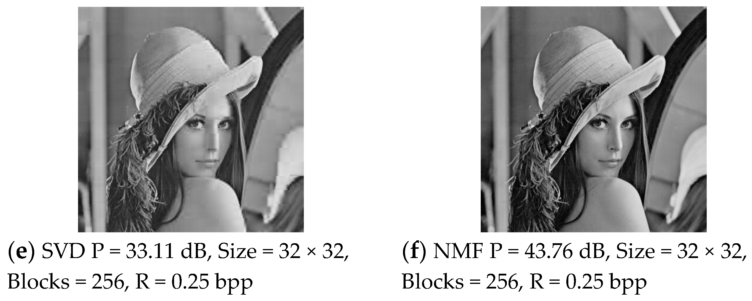
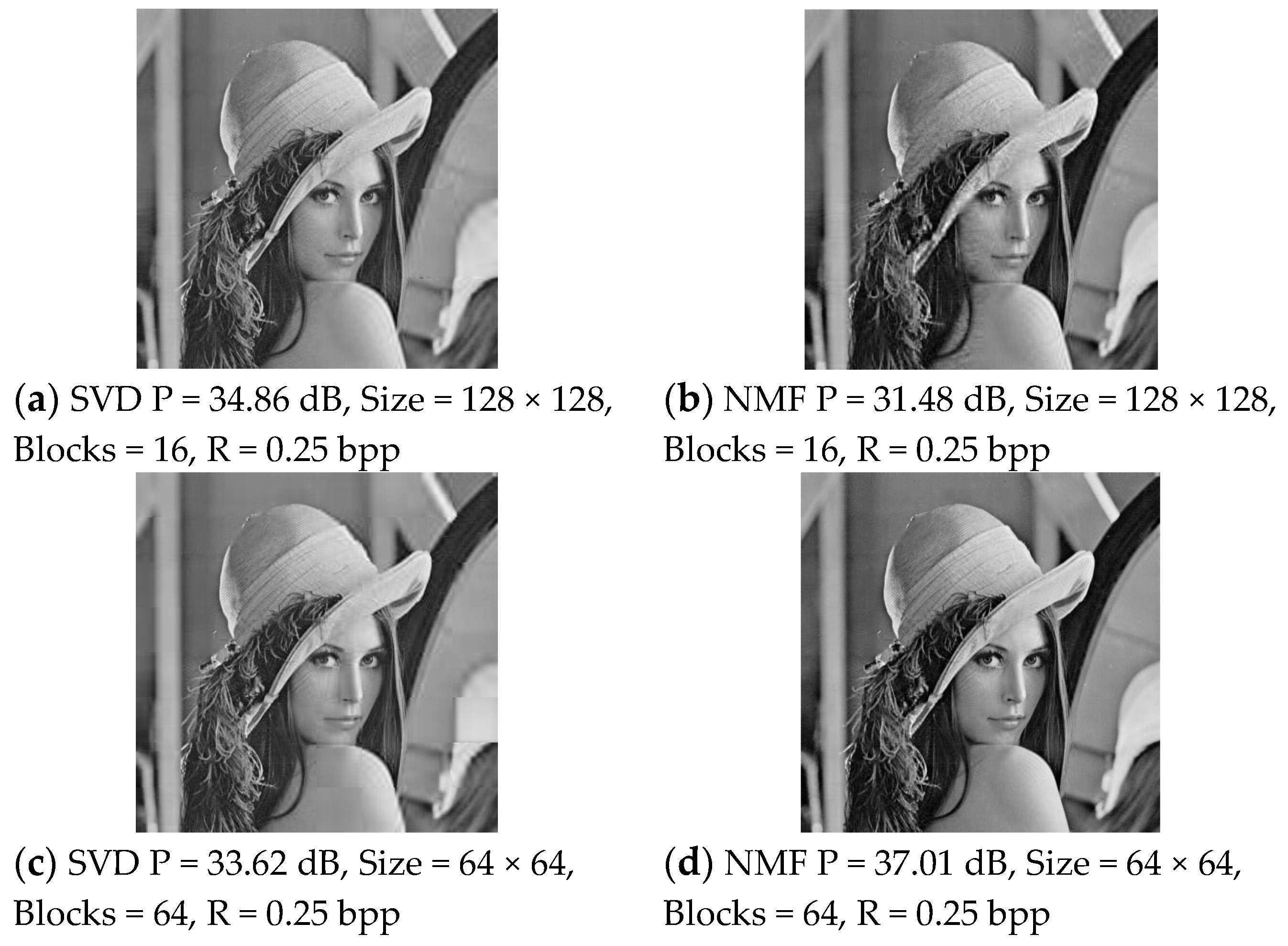
4.2.1. Impact on Compression Mechanism Caused by Image Blocks

Table 1 lists the quality of image restoration under different number of iterations (I) and blocks (B) respectively.
In Table 1, if the iteration is a constant and compression ratio is set to 0.25 bpp, the P is greater when the number of sub-blocks is greater. At the same time, P’s growth rate becomes slower which is inferred from the diminishing characteristic on ( 0 , + ) . That is, when the number of blocks is large, the image restoration quality does not necessarily become better than the small numbers.
Especially, for the image block compression and restoration algorithms, a significant growth (e.g., 1st column) of P from 26.88 to 43.76 shows that the number of image blocks plays an important role in the compression scheme. This may be one of the key issues and provide us with new ideas when doing further research in this method.

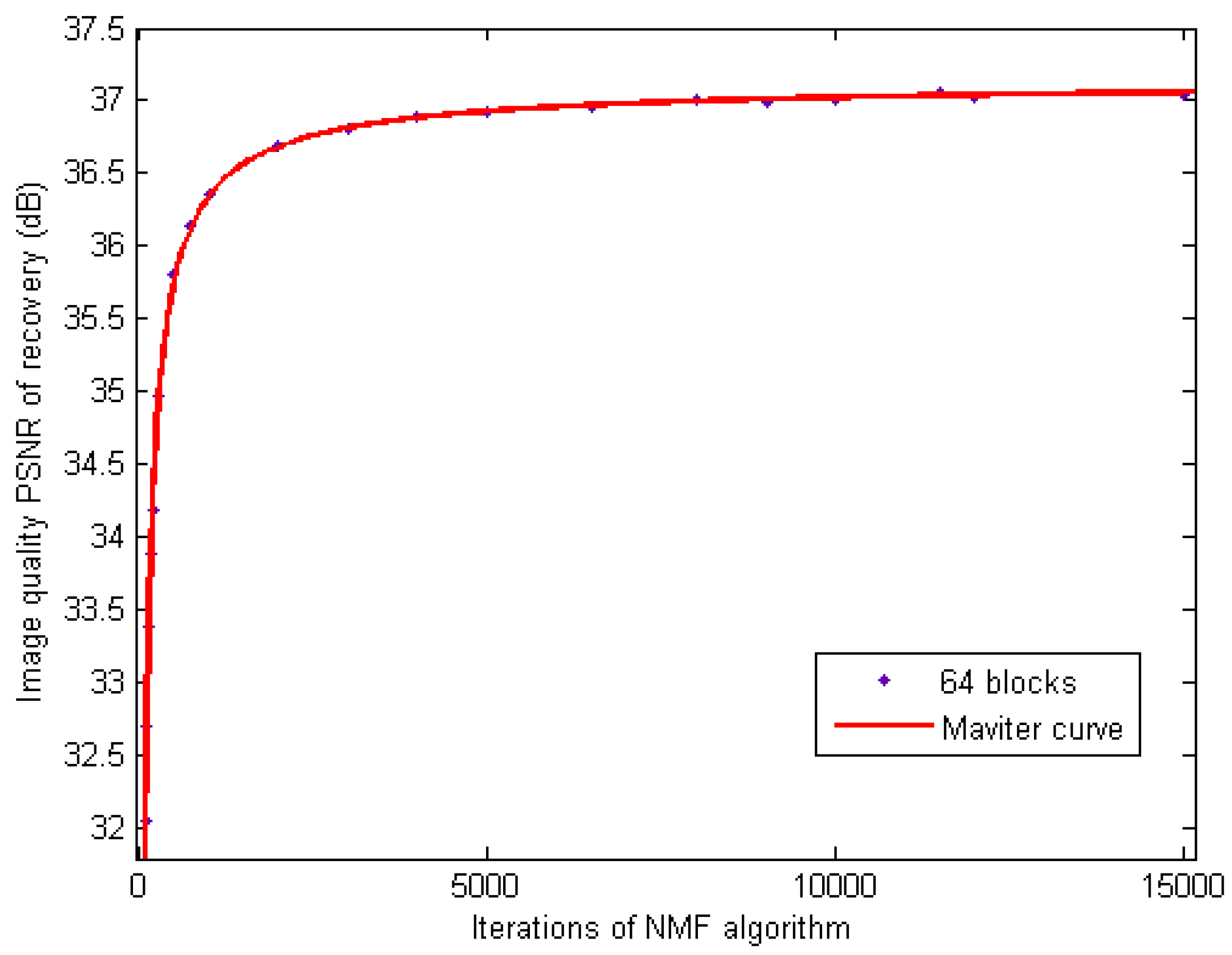
4.2.2. Impact on Compression Mechanism Caused by Iterations

Table 2 lists the quality of image restoration under different iterations when the number of blocks is 64. We use MATLAB to carry out the fitting of data in Figure 4.
As is shown in Figure 4, if the number of blocks is a constant, the P increases with the rise of iteration quickly when the iteration is small. When the iteration becomes very large, the P increases slowly and approaches a limit. This phenomenon is essential for further study as the fitting curve looks like an exponential curve.
Considering the energy consumption makes a critical difference in the whole compression scheme in WMSNs and the mathematical results above, the iteration is another key point of this method. Combining with these relations, we need to select an appropriate number of blocks and iterations in order to get moderate image quality while taking the time consumption of the algorithm into consideration.

4.3. Compression with Other Methods

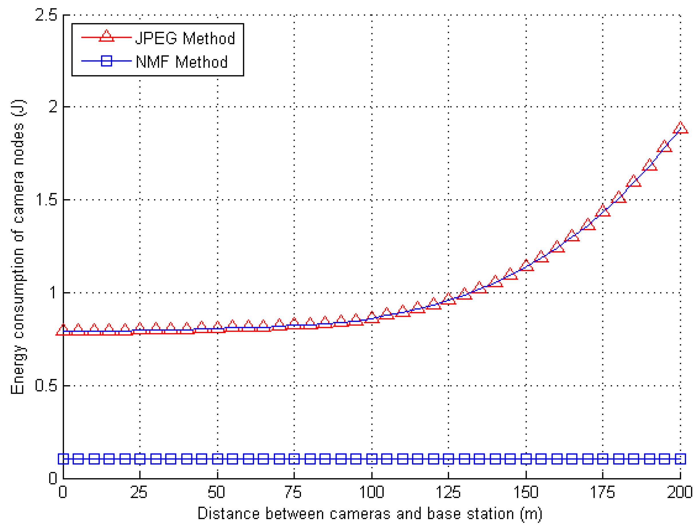
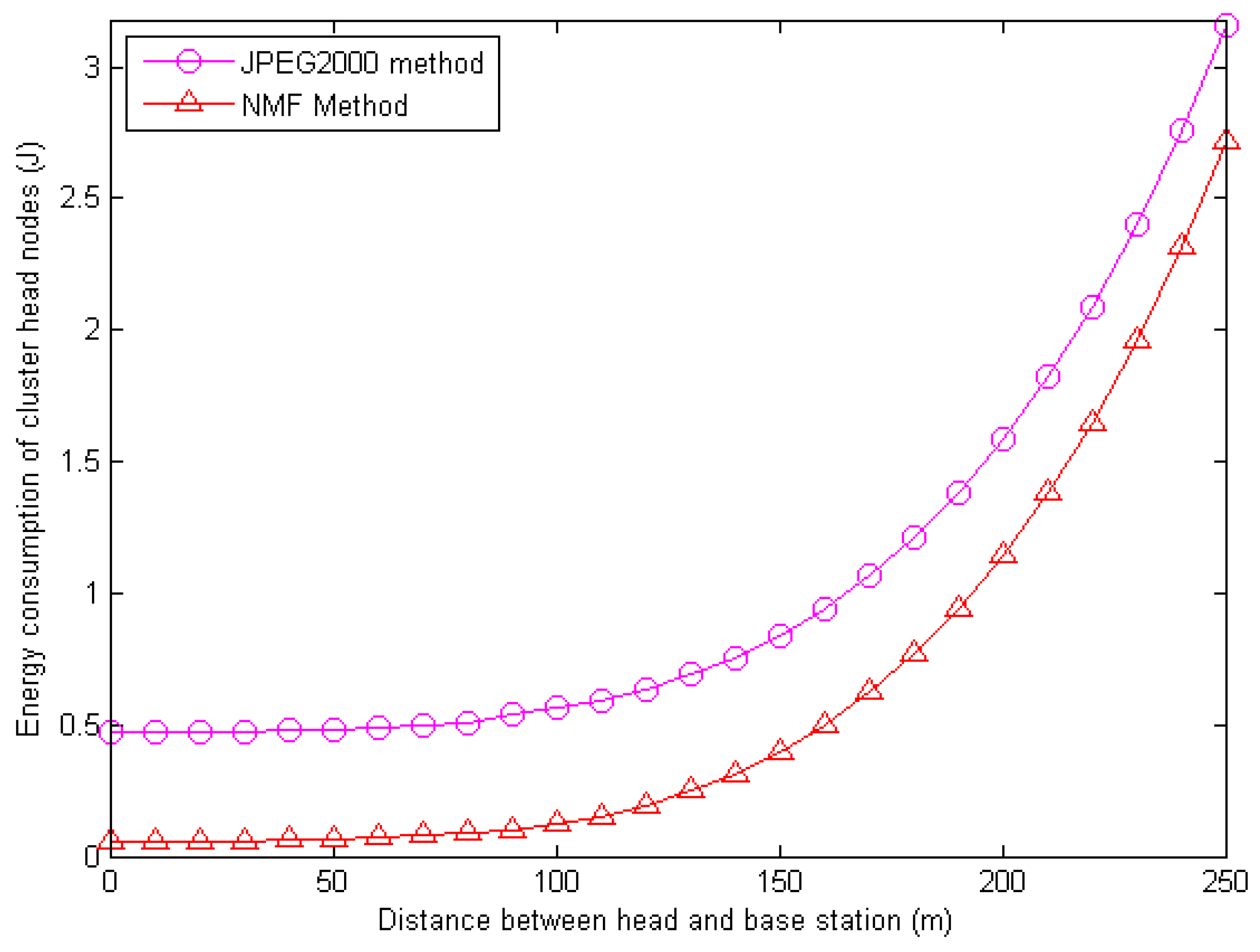
4.3.1. Analysis of Energy Consumption

Figure 5 is a comparison between centralized and collaborative image compression transmission schemes. It is an energy distribution figure when sending a 512 × 512 × 8-bit image to the base station. The simulation result shows that the use of the collaborative method described in this paper reduces the average energy consumption of the camera nodes by nearly an order of magnitude lower than the centralized approach. The energy consumption of nodes has a strong balance, which is helpful to improve lifetime of network and extend the life cycle.
Figure 6 shows the energy consumption of the cluster head node using the JPEG2000 method [21] and the NMF method.
In Figure 6, the energy consumption of the cluster head node using the method in this paper is obviously lower than the JPEG2000 method.
Because the energy consumption of the JPEG2000 method contains three parts and the energy consumption of the method in this paper contains only one part (the energy consumption in accepting data from the ordinary nodes and transferring received data to the base station), it costs less energy consumption.
We made a comparison of the energy consumption of camera nodes at the same time, as is shown in Figure 7. In this paper, cameras are only responsible for transferring blocks to ordinary nodes within a communication range at a certain probability. In the JPEG2000 algorithm mechanism, cameras are also responsible for the image preprocessing, calculating the gradient amplitude of image edge information and transferring image blocks to the cluster heads. Therefore, the total energy consumption of each node in this paper is less than in the JPEG2000 compression mechanism under the same condition.

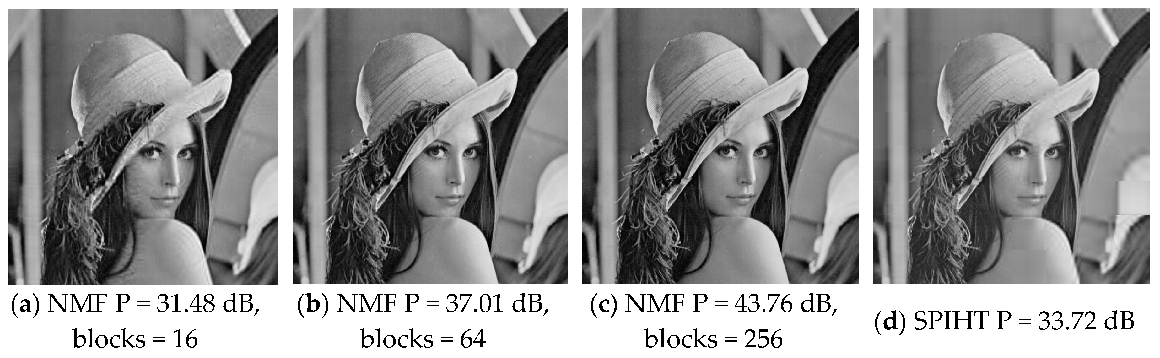
4.3.2. Quality of Image Restoration

Energy consumption of the SVD compression mechanism is partly consistent with the NMF method. However, in terms of image restoration quality, when numbers of image blocks exceed a certain value, the obtained quality in this paper is much higher than the SVD compression mechanism, as can be seen from Figure 1 in Chapter 3.1. Table 3 lists a comparison of image restoration quality with unit of dB (Signal-to-Noise ratio) between the SVD method and the NMF method.
From Table 3, we can see that, although the SVD method and the NMF method are both distributed compression mechanism, the NMF method has a more remarkable quality of image restoration under the same block numbers with the SVD method. Moreover, the NMF method can obtain the same effect as the SVD method by fewer iterations. Meanwhile, although the SPIHT method has a slight advantage over the SVD method, it does not show a better performance of the NMF method.
At the same time, we noted that in the SVD mechanism, the smaller image blocks are (i.e., the more image blocks are divided), the increasing artifacts and edge effect are more obvious and the lower image restoration quality is. Taking the above into consideration, this paper proposed a collaborative image processing method which has a lower energy consumption than the JPEG2000 and a higher image restoration quality than the SVD cooperative image processing method and the SPIHT method do.

5. Conclusions

In this paper, we studied the issue of image compression and transmission in WMSNs. Considering the data processing and energy distribution characteristics in WMSNs practical applications, we adopt the NMF method to compress and transfer images based on the collaboration of nodes in the whole system. Furthermore, we made nodes responsible for different functions, such as data processing and data transmission over long distances, respectively. This makes the energy consumption of the whole system become homogenic. Simulation results show that the proposed NMF-based image compression mechanism can alleviate the energy consumption of camera nodes which are the key roles in the network. At the same time, it can balance the energy consumption of the whole network and extend the lifetime. It can also effectively eliminate the common noise and improve the image restoration quality.

Acknowledgments

This work is supported by the National Natural Science Foundation of China under Grant No. 61572261, the Natural Science Foundation of Jiangsu Province under Grant No. BK20150868, the China Postdoctoral Science Foundation funded project under Grant No. 2014M551635, the Jiangsu Planned Projects for Postdoctoral Research Funds under Grant No. 1302085B, the NUPTSF under Grant No. NY214013, the Open Fund for the Key Laboratory for Traffic and Transportation Security of Jiangsu Province under Grant No. TTS201502.

Author Contributions

Shikang Kong mainly designed the research scheme and wrote the paper. Lijuan Sun supervised the work. Chong Han performed the research and wrote the paper. Jian Guo obtained and analyzed the data. All the authors have read and approved the final manuscript.

Conflicts of Interest

The authors declare no conflict of interest.

References

  1. Akyildiz, I.F.; Melodia, T.; Chowdhury, K.R. A survey on wireless multimedia sensor networks. Comput. Netw. 2007, 51, 921–960. [Google Scholar] [CrossRef]
  2. Gurses, E.; Akan, O.B. Multimedia communication in wireless sensor networks. Ann. Telecommun. 2005, 60, 799–827. [Google Scholar]
  3. Wei, Z.; Wang, F. A Novel Negative Multinomial Distribution Based Energy-Efficient Reputation Modeling for Wireless Sensor Networks (WSNs). J. Donghua Univ. (Eng. Ed.) 2012, 29, 153–156. [Google Scholar]
  4. Xiong, Z.Y. Study of Image Coding Algorithm for Wireless Multimedia Sensor Networks. Ph.D. Thesis, Central South University, Changsha, China, 2012. [Google Scholar]
  5. Addisu, A.; Sciandra, V.; Agueh, M.; George, L. Work in progress: Analytic hierarchy process applied to JPEG2000 video streaming over Wireless Multimedia Sensor Networks. In Proceedings of the IEEE 2014 9th International Conference on Communications and Networking in China (CHINACOM), Maoming, China, 14–16 August 2014; pp. 361–364.
  6. Han, C.; Sun, L.; Xiao, F.; Guo, J.; Wang, R. Image compression scheme in wireless multimedia sensor networks based on SVD. J. Southeast Univ. (Nat. Sci. Ed.) 2012, 42, 814–819. [Google Scholar]
  7. Lee, D.D.; Seung, H.S. Learning the parts of objects by non-negative matrix factorization. Nature 1999, 401, 788–791. [Google Scholar] [PubMed]
  8. Wang, J.; Du, H.; Hou, Y.; Jin, Y. Graph embedding projective non-negative matrix factorization method for image feature extraction. Comput. Sci. 2014, 41, 311–315. (In Chinese) [Google Scholar]
  9. Zhang, W.; Guan, N.; Tao, D.; Mao, B.; Huang, X.; Luo, Z. Correntropy supervised non-negative matrix factorization. In Proceedings of the IEEE 2015 International Joint Conference on Neural Networks (IJCNN), Killarney, Ireland, 12–17 July 2015; pp. 1–8.
  10. Donoho, D.L.; Stodden, V. When does non-negative matrix factorization give a correct decomposition into parts? In Advances in Neural Information Processing Systems 16 (NIPS 2003); MIT Press: Cambridge, MA, USA, 2003. [Google Scholar]
  11. Kumar, A.; Sindhwani, V.; Kambadur, P. Fast Conical Hull Algorithms for Near-separable Non-negative Matrix Factorization. JMLR W&CP 2013, 28, 231–239. [Google Scholar]
  12. Lee, D.D.; Seung, H.S. Algorithms for non-negative matrix factorization. In Advances in Neural Information Processing Systems 13; MIT Press: Cambridge, MA, USA, 2001; pp. 556–562. [Google Scholar]
  13. Lin, C.J. Projected gradient methods for non-negative matrix factorization. Neural Comput. 2007, 19, 2756–2779. [Google Scholar] [CrossRef] [PubMed]
  14. Huang, K.; Sidiropoulos, N.; Swami, A. Non-negative matrix factorization revisited: Uniqueness and algorithm for symmetric decomposition. IEEE Trans. Signal Process. 2014, 62, 211–224. [Google Scholar] [CrossRef]
  15. Wang, K.-J.; Zuo, C.-T. Improvements of non-negative matrix factorization for image extraction. Appl. Res. Comput. 2014, 31, 4. (In Chinese) [Google Scholar]
  16. Ehsan, S.; Hamdaoui, B. A survey on energy-efficient routing techniques with QoS assurances for wireless multimedia sensor networks. IEEE Commun. Surv. Tutor. 2012, 14, 265–278. [Google Scholar] [CrossRef]
  17. Heizelman, W.; Chandrakasan, A.; Balakrishman, H. Energy-Efficient communication protocol for wireless microsensor networks. In Proceedings of the Hawaiian International Conference on System Science (HICSS), Maui, HI, USA, 4–7 January 2000; IEEE Press: Washington, DC, USA, 2000; pp. 3005–3014. [Google Scholar]
  18. Wang, A.; Chandrakasan, A. Energy-efficient DSPs for wireless sensor networks. IEEE Signal Process. Mag. 2002, 19, 68–78. [Google Scholar] [CrossRef]
  19. Jin, Y.; Wang, L.; Yang, X.; Wen, D. Energy Consumption in Wireless Sensor Networks. J. Donghua Univ. (Eng. Ed.) 2007, 24, 646–651. [Google Scholar]
  20. Wheeler, F.W.; Pearlman, W.A. SPIHT image compression without lists. In Proceedings of the IEEE 2000 International Joint Conference on Acoustics, Speech, and Signal Processing (ICASSP’00), Istanbul, Turkey, 5–9 June 2000; Volume 42, pp. 2047–2050.
  21. Lu, Q.; Luo, W.S.; Hu, B. Multi-node cooperative JPEG2000 implementation based on neighbor clusters in wireless sensor networks. Opt. Precis. Eng. 2010, 18, 240–247. (In Chinese) [Google Scholar]
Figure 1. Reconstructed image contrast between NMF & SVD compression method.
Information 08 00026 g001aInformation 08 00026 g001b
Figure 2. Comparison between NMF (with different block numbers) & SPIHT compression method.
Information 08 00026 g002
Figure 3. Network structure of collaborative compression mechanism.
Information 08 00026 g003
Figure 4. Fitting curve of iterations and Peak Signal to Noise Ratio (PSNR) with 64 blocks.
Information 08 00026 g004
Figure 5. (a) Energy distribution of centralized image compression network; (b) Energy distribution of collaborative image compression network.
Information 08 00026 g005
Figure 6. Energy consumption of cluster head nodes in different methods.
Information 08 00026 g006
Figure 7. Energy consumption of camera nodes in different methods.
Information 08 00026 g007
Table 1. Quality of image under different iterations and blocks.
I = 1000I = 5000I = 10000
BP (dB)BP (dB)BP (dB)
426.88427.12427.13
1631.181631.451631.48
6436.366436.926437.02
25643.7625645.6325645.93
Table 2. Quality of image under different iterations with 64 blocks.
IP (dB)IP (dB)
10032.04300036.81
12032.70400036.89
15033.39500036.92
18033.89650036.96
20034.18800037.00
30034.97900036.99
50035.811000037.01
75036.1411,50037.05
100036.3612,00037.03
200036.6915,00037.04
Table 3. Comparison of image quality.
BINMF (dB)SVD (dB)SPIHT (dB)
6410032.0433.6233.72
15033.39
20034.18
30034.97
50035.81
2561024.8333.11
3030.44
5033.34
7535.38
10036.77

