An Effective and Robust Single Image Dehazing Method Using the Dark Channel Prior

Abstract

In this paper, we propose a single image dehazing method aiming at addressing the inherent limitations of the extensively employed dark channel prior (DCP). More concretely, we introduce the Gaussian mixture model (GMM) to segment the input hazy image into scenes based on the haze density feature map. With the segmentation results, combined with the proposed sky region detection method, we can effectively recognize the sky region where the DCP cannot well handle this. On the basis of sky region detection, we then present an improved global atmospheric light estimation method to increase the estimation accuracy of the atmospheric light. Further, we present a multi-scale fusion-based strategy to obtain the transmission map based on DCP, which can significantly reduce the blocking artifacts of the transmission map. To further rectify the error-prone transmission within the sky region, an adaptive sky region transmission correction method is also presented. Finally, due to the segmentation-blindness of GMM, we adopt the guided total variation (GTV) to tackle this problem while eliminating the extensive texture details contained in the transmission map. Experimental results verify the power of our method and show its superiority over several state-of-the-art methods.

1. Introduction

Due to the atmospheric suspended particles that absorb and scatter the light before reaching the camera, outdoor images are significantly degraded by bad weather conditions (fog, haze, etc.) and yield a poor visual effect, including the reduced contrast, faint color and blurred scene details. This is a major problem for most applications of computational photography and computer vision, such as satellite imaging, object recognition, intelligent vehicles, etc., since they are primarily designed under the assumption that the input images have clear visibility. Thus, removing the negative visual effects and unveiling the true scene, which is often referred to as “dehazing”, is highly desired and has strong implications. However, dehazing is a challenging ill-posed problem due to the variety of densities, types and distributions of atmospheric suspended particles, as well as the polarization states of the ambient incident light [1].

Recently, benefiting from the atmospheric scattering model proposed by Narasimhan and Nayar [1,2,3], many single image dehazing methods have been proposed [1,2,3,4,5,6,7,8,9,10,11,12,13,14,15,16,17,18,19,20,21,22,23,24], and significant progress has been made. These model-based methods estimate the values of the model coefficients by taking the hazy image degradation mechanism into consideration and, therefore, eliminate the negative effects and recover the scene albedo. In general, the success of the model-based methods lies in utilizing priors/assumptions; however, limitations may appear when the priors/assumptions are invalid under some specific conditions. For instance, Tan [4] enhances the visibility of hazy images by manipulating the contrast based on the assumption that the recovered image has higher contrast than the relevant plagued image. However, the restored image tends to be over-saturated and inevitably suffers from block artifacts. Tarel et al. [10] estimate the veil by using combinations of filters and obtain a contrast enhanced image. Despite the advantage of linear complexity, haze remains where the depth changes drastically because the median filter involved provides poor edge-preserving performance. Although Fattal’s method [5] can produce impressive results by assuming that the surface shading is uncorrelated with the scene transmission within a local patch, this method is invalid for dense haze image since the assumption is broken in this case. Zhu et al. [6] discover the color attenuation prior (CAP) and removed haze by creating a linear model for modeling the depth structure. Nevertheless, this method is proven to be invalid for a dense haze image where the prior is invalid. Similar to Zhu et al.’s method, Ju et al. [8] establish a linear model for transmission estimation, which enables us to directly obtain the transmission map, but this method cannot apply to dense haze images due to the insufficient training samples.

Remarkably, He et al. propose the sound DCP [7], which allows us to directly estimate the rough transmission based on the atmospheric scattering model. Although this DCP is physically valid in general and can recover a visually-pleasing image, two main inherent limitations still exist. That is, the sky regions tend to be over-enhanced, and the global edge-consistency is prone to be inaccurate, as we note in Section 2.

Consequently, several relevant improvements have been proposed aiming at overcoming these limitations [12,13,14,15,18,19,25,26,27,28]. For example, in order to avoid the over-enhancement within the sky regions, Shi et al. [27] design a rough sky region estimation method to detect the region where the DCP may fail and adjust the transmission map by comparing the average intensity of the detected sky region with the value of the global atmospheric light. However, this method has its limitations when processing dense haze images since it may yield a false interpretation of objects shrouded in dense haze as sky regions. Li et al. [28] obtain the sky region based on the proposed sky region prior and color edge detection and create a color normalization method to refine the transmission within the sky regions. Nevertheless, the exceptional process may not satisfy minor non-sky-region images. Ju et al. [15] design a sky region identification method using dual thresholds and further correct the corresponding transmission within the sky regions, but the fixed threshold cannot be applied to various types of haze images. On the other hand, to refine the transmission, which is obtained via DCP, the soft matting technique is adopt in [7], whereas the computational efficiency is relatively low and therefore cannot be applied to real-time processing. Consequently, several filtering-based methods are proposed to improve the efficiency of the transmission refinement, including the bilateral filter [19], guided filter [26] and guided joint bilateral filter [12]. Although the efficiency of [12,19,26] is much higher compared with the soft matting technique, the dehazing effect is unstable since these filtering-based methods may be parameter sensitive, as discussed in [11].

In this paper, we propose a single image dehazing method aiming at overcoming the inherent limitations of DCP. Compared with the previous methods, our method has several advantages: (1) benefitting from the sky region detection method, we can precisely recognize the sky region and further increase the estimation accuracy of atmospheric light via the proposed global atmospheric light estimation method; (2) to obtain a more accurate transmission map, we present a multi-scale transmission map fusion method to blend seamlessly two transmission maps that are estimated via DCP with different patch sizes and further rectify the error-prone transmission within the sky region via the proposed adaptive sky region transmission correction method; (3) we adopt the guided total variation (GTV) model to smooth the edge between the sky region and the adjacent areas aiming at compensating the segmentation-blindness of GMM; meanwhile, the extensive texture details in the transmission map can be effectively eliminated.

2. Related Work

2.1. Atmospheric Scattering Model

When light passes through the hazy atmospheric media, light that reflected from objects is attenuated and scattered along the path to the sensor. Mathematically, the degradation procedure can be described via the widely-used atmospheric scattering model [1,2,3], which can be expressed as follows:

$$I\left(x,y\right)=L_{\infty }\cdot \mathsf{\rho }\left(x,y\right)\cdot e^{-\beta \cdot d\left(x,y\right)}+L_{\infty }\cdot \left(1-e^{-\beta \cdot d\left(x,y\right)}\right)$$

(1)

where $\left(x,y\right)$ is the pixel index, $I\left(x,y\right)$ is the degraded hazy image, $L_{\infty }$ is the global atmospheric light, which is an RGB vector that describes the intensity of the scattered light, $\mathsf{\rho }\left(x,y\right)$ is the scene albedo, $\beta$ is the scattering coefficient and $d\left(x,y\right)$ is the scene depth. For expression simplicity, we use $J\left(x,y\right)=L_{\infty }\cdot \mathsf{\rho }\left(x,y\right)$ and $t\left(x,y\right)=e^{-\beta \cdot d\left(x,y\right)}$ to represent the corresponding recovered image and transmission, respectively. Thus, Equation (1) can be rewritten as:

$$I\left(x,y\right)=J\left(x,y\right)\cdot t\left(x,y\right)+L_{\infty }\cdot \left(1-t\left(x,y\right)\right)$$

(2)

Generally, the single image dehazing method is an inverse problem that predicts all of the corresponding unknown coefficients using the input hazy image $I\left(x,y\right)$ and further recovers the image $J\left(x,y\right)$.

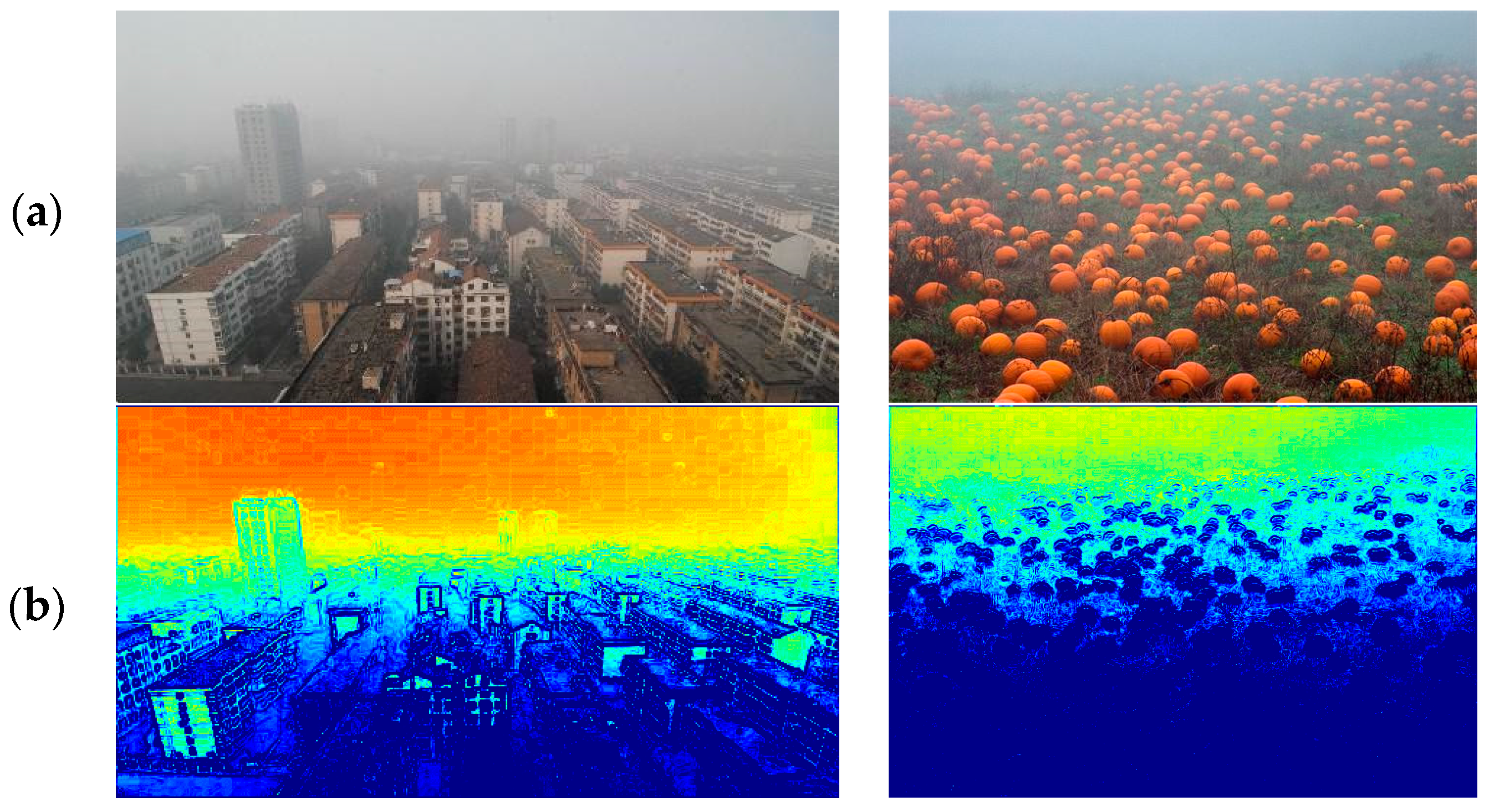
2.2. Analysis of DCP Limitations

The DCP is proposed by He et al. [7], which is a kind of statistics of extensive haze-free outdoor images, that is within most local patches (except for the sky region), at least one color channel contains the pixel whose intensity is extremely low and tends to be zero, and it can be expressed as:

$$J^{dark}\left(x,y\right)=\underset{c\in \{r,g,b\}}{\min }\left(\underset{\left(x^{\prime },y^{\prime }\right)\in \mathsf{\Omega }\left(x,y\right)}{\min }\left(J^c\left(x^{\prime },y^{\prime }\right)\right)\right)\to 0$$

(3)

where $c$ is the RGB color channel index, $\mathsf{\Omega }\left(x,y\right)$ is a local patch centered at $\left(x,y\right)$ and $J^c\left(x,y\right)$ and $J^{dark}\left(x,y\right)$ are the color channel and dark channel that correspond to image $J\left(x,y\right)$, respectively.

This prior, combined with the atmospheric scattering model, enables us to directly estimate the rough transmission for a hazy image. Despite the effectiveness of this prior, the image restored via DCP is prone to suffer from the over-enhanced sky region, as well as the poor global edge-consistency. Generally, the reason can be explained as follows: (1) DCP fails for the region where the scene brightness is similar to the atmospheric light (such as the sky region), since the dark channel that corresponds to the sky region is obviously higher than zero, and therefore, the transmission will be inevitably over-estimated if we apply the DCP directly; (2) DCP is a patch-based procedure; thus, the transmission map that is estimated via DCP may suffer from the poor edge-consistency property, and this problem will further lead to negative visual effects in the corresponding restored image.

3. Single Image Dehazing Method

In this section, we propose a single image dehazing method aiming at overcoming the inherent limitations of DCP; the main procedures are illustrated in Figure 1. Inherently inspired by [16,22], we detect the sky region based on the haze density feature map and scene segmentation technique. Then, we apply three key steps, including the improved global atmospheric light estimation, the multi-scale transmission map fusion and the adaptive sky region transmission correction. Next, we introduce the guided total variation (GTV) to smooth the edge around the sky region and eliminate the extensive texture details in the transmission map. Finally, with the knowledge of global atmospheric light and the transmission map, the image can be recovered via the atmospheric scattering model.

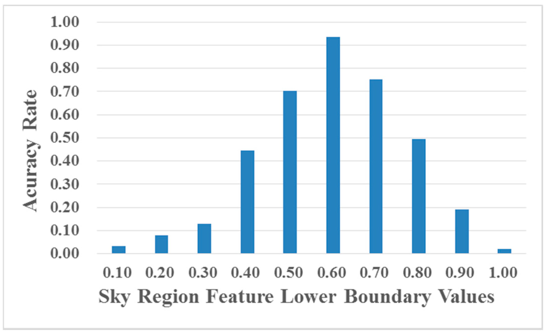
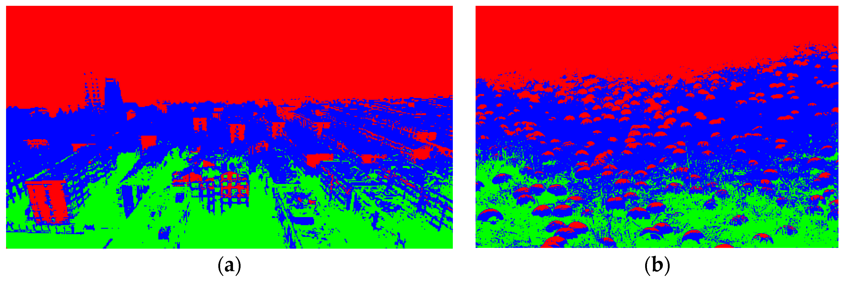
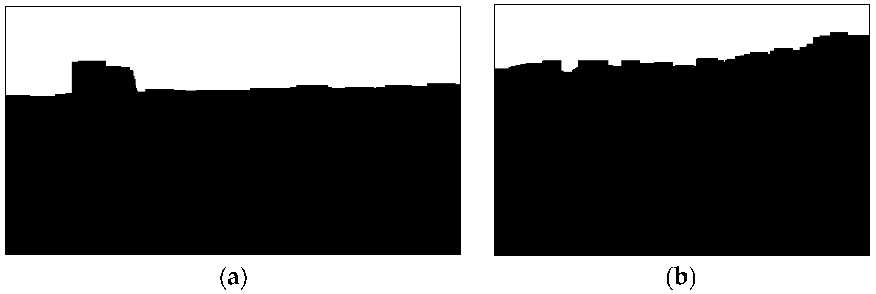
3.1. Sky Region Detection via Scene Segmentation

As discussed by [6,7,11], DCP may be invalid for a sky region where the brightness of the scene object is inherently similar to the air light. Therefore, inspired by [16,22], we introduce the haze density feature map [16] and the GMM model [29] to segment a hazy image into scenes and further recognize the sky region via the proposed sky region detection method. The detailed procedures are demonstrated as follows.

(a) Haze density feature map:

Considering the fact that the hazy images are subjected to the blurred object details, reduced contrast and fade surface color, thus it is difficult to directly segment a hazy image into scenes via scene features extraction. However, according to the atmospheric scattering model, the magnitude of degradation for a hazy image is proportional to the haze density. That is, the most haze-opaque regions should have the highest brightness and the most blurred details, and vice versa. Thus, we introduce the haze density prediction model [16] to describe the haze density feature map as:

$$\{\begin{array}{c}S(x,y)=\alpha \cdot Q_L(x,y)-\beta \cdot Q_T(x,y)\\ Q_L(x,y)=\frac{1}{\left|\mathsf{\Omega }\right|}\cdot {\displaystyle \sum _{(x\prime ,y\prime )\in \mathsf{\Omega }(x,y)}{L}_I(x\prime ,y\prime )}\\ Q_T(x,y)=\frac{1}{\left|\mathsf{\Omega }\right|}\cdot {\displaystyle \sum _{(x\prime ,y\prime )\in \mathsf{\Omega }(x,y)}\left|\nabla I(x\prime ,y\prime )\right|}\end{array}$$

(4)

where $S\left(x,y\right)$ is the haze density feature map; $\alpha =1.126$ and $\beta =0.705$ are the regularization coefficients that are used to adjust the significance of each component; $Q_L(x,y)$ and $Q_T(x,y)$ are the brightness feature index and texture detail feature index of a hazy image $I\left(x,y\right)$, respectively; $L_I(x,y)$ and $\nabla I(x,y)$ are the brightness component and the gradient component that correspond to a hazy image $I\left(x,y\right)$, respectively; $\mathsf{\Omega }\left(x,y\right)$ is the local patch which is centered at $\left(x,y\right)$;, and $\left|\mathsf{\Omega }\right|$ is the corresponding pixel number within this local patch.

In Figure 2, Figure 2a shows two hazy images and Figure 2b demonstrates the corresponding haze density feature maps. In can be noticed that the obtained haze density feature map can precisely describe the spatial relationship of the haze density distribution and is well consistent with visual perception of haze density

(b) Scene segmentation:

On the basis of the haze density feature map $S\left(x,y\right)$, we need to segment the hazy image into scenes, and pixels within a segmented scene should share approximately the same scene feature after segmentation. Thus, we convert the scene segmentation into the clustering problem. Considering the accuracy requirement and the computational cost, we introduce the Gaussian mixture model (GMM) [29] to conduct the segmentation procedure. According to [29,30], the GMM can be described via a K Gaussian component mixing model, and the relevant probability density function is expressed as:

$$p\left(S\left(x,y\right)\right)={\displaystyle \sum _{k=1}^{K}p\left(k\right)p\left(S\left(x,y\right)|k\right)={\displaystyle \sum _{k=1}^K{\pi }_{k}N\left(S\left(x,y\right)|{\mu }_k,{\sigma }_k\right)}}$$

(5)

where $S\left(x,y\right)$ is the obtained haze density feature map and $\left\{{\pi }_k,{\mu }_k,{\sigma }_k\right\}$ are the mixing proportion, mean and variance of the k-th component of GMM, respectively. The relevant log-likelihood function of Equation (5) is:

$$\lambda ={\displaystyle \sum _{x=1}^{l_w}{\displaystyle \sum _{y=1}^{l_h}\log \left\{p\left(S\left(x,y\right)\right)\right\}}}$$

(6)

where $l_w$ and $l_h$ are the width and height of $S$, respectively. We further adopt an expectation-maximization (EM) strategy to determine the model parameter $\left\{{\pi }_k,{\mu }_k,{\sigma }_k\right\}$ aimed at maximizing the log-likelihood function. Therefore, the posteriori probability $\omega (S(x,y),k)$ is defined as:

$$\omega (S(x,y),k)=\frac{{\pi }_{k}N\left(S\left(x,y\right)|{\mu }_k,{\sigma }_k\right)}{{\displaystyle {\sum }_{i=1}^K{\pi }_{k}N\left(S\left(x,y\right)|{\mu }_i,{\sigma }_i\right)}}$$

(7)

Then, we compute the model parameter $\left\{{\pi }_k,{\mu }_k,{\sigma }_k\right\}$ as:

$$\{\begin{array}{l}{\pi }_k=N_k/res\hfill \\ {\mu }_k=\frac{1}{N_k}{\displaystyle \sum _{x=1}^{l_w}{\displaystyle \sum _{y=1}^{l_h}\omega \left(S\left(x,y\right),k\right)S\left(x,y\right)}}\hfill \\ {\sigma }_k=\frac{1}{N_k}{\displaystyle \sum _{x=1}^{l_w}{\displaystyle \sum _{y=1}^{l_h}\omega \left(S\left(x,y\right),k\right)\left(S\left(x,y\right)-{\mu }_k\right){\left(S\left(x,y\right)-{\mu }_k\right)}^T}}\hfill \\ N_k={\displaystyle \sum _{x=1}^{l_w}{\displaystyle \sum _{y=1}^{l_h}\omega \left(S\left(x,y\right),k\right)}}\hfill \end{array}$$

(8)

where $res=l_w\cdot l_h$ denotes the number of pixels of $S$. This procedure is computed iteratively and terminates when the likelihood function converges.

Note that, the segmentation accuracy is generally proportional to the value of $K$ according to Equation (5); nevertheless, the computational cost is another important concern. After repeated testing, we take $K=3$ as a balanced choice for our method. The corresponding scene segmentation results for Figure 2 are displayed in Figure 3.

(c) Sky region detection:

Now that we have segmented the hazy image into $K$ scenes and the corresponding pixel index sets are denoted as $\left\{\Delta \left(k\right),k\in \left[1,K\right]\right\}$, then we will detect the sky region within these scenes based on two considerations: (1) by means of the haze density feature map, the sky region (which is the most haze-opaque region) should have the highest average scene feature value among all of the segmented scenes; (2) in fact, a few particular outdoor images do not contain the sky scene, which may cause errors if we simply correct the transmission within the scene with the highest feature value; thus, it is necessary to detect and exclude this special situation. Consequently, we create the sky region detection method as follows:

$${\Delta }_{sky}=\{\begin{array}{c}\widehat{\Delta }mean\left(S\left(\widehat{\Delta }\right)\right)\ge T_{1}and\frac{\left|\Delta \left(k\right)\right|}{res}\ge T_2\\ \varnothing else\end{array}$$

(9)

where $\widehat{\Delta }=\arg \underset{k}{\max }\left\{\frac{{\displaystyle {\sum }_{\left(x,y\right)\in \Delta \left(k\right)}S\left(x,y\right)}}{\left|\Delta \left(k\right)\right|}\right\},k\in \left[1,K\right]$ is the candidate sky region, which has the highest feature value, $T_1$ is the lower boundary of sky region feature and $T_2$ is the lower boundary of the scene area ratio.

According to our previous work [16], we set $T_2=0.2$ as the value of lower boundary of the scene area ratio. More specifically, we conduct extensive experiments to determine the relatively balanced selection of the lower boundary of sky region feature $T_1$. We randomly collect 200 hazy images from the Internet and obtain the accuracy rate of sky region detection (compared with human-rate judgement) using different values of the sky region feature lower boundary $T_1$ (0.1–0.9) and provide the corresponding statistic results in Figure 4. From Figure 4, we can notice that the highest accuracy rate of sky region detection can be achieved when $T_1=0.6$.

In addition, for the purpose of eliminating the clustering error and the high light noise, we further utilize the erosion operator of mathematical morphology [31] to refine the scene segmentation result before we detect the sky region. As shown in Figure 5, we can effectively detect the sky region for Figure 2 and mark it as white.

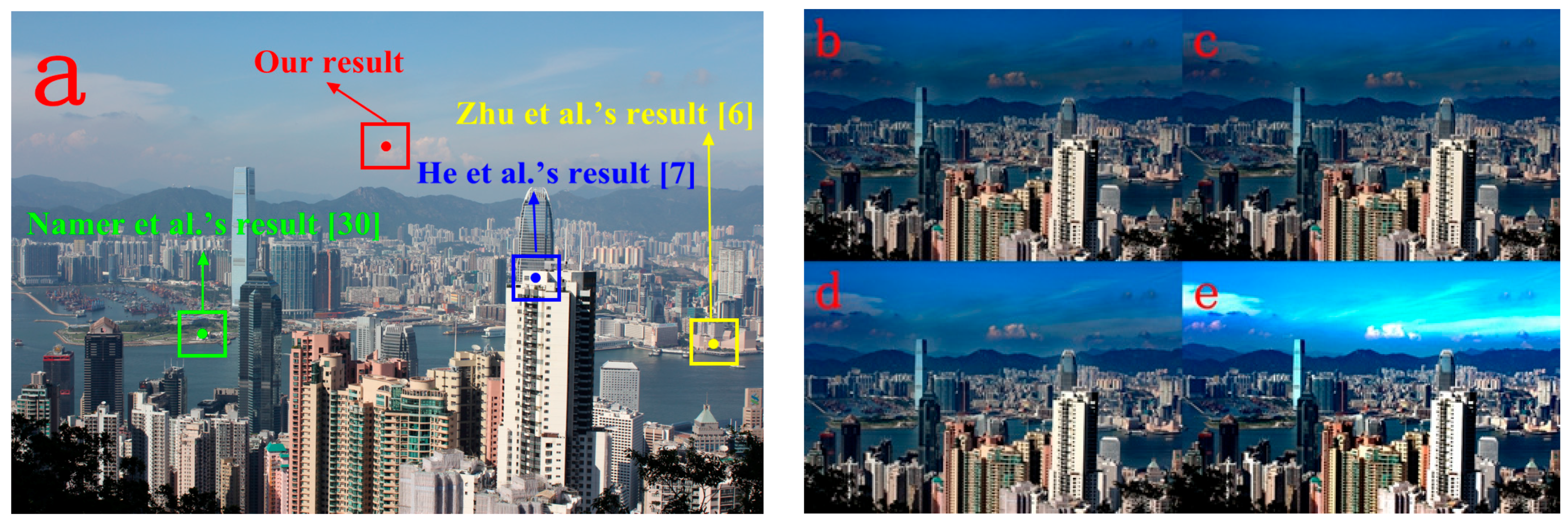
3.2. Improved Global Atmospheric Light Estimation Method

In existing dehazing methods, the global atmospheric light is either located manually or estimated using basic procedures that take the brightest pixel of the hazy image [32,33]. In fact, it is error prone to simply locate the brightest pixel of the hazy image, since it may belong to an interference object (white/gray objects, high-light, extra light source, etc.).

To increase the precision of global atmospheric light location, several improvements have been proposed. For instance, He et al. [7] pick the top 0.1% brightest pixels in the dark channel, which is estimated via DCP and take the pixel with highest intensity among these pixels as the atmospheric light. Zhu et al. [6] select the top 0.1% brightest pixels in the depth map, which is obtained via the color attenuation prior (CAP), and take the pixel with the highest intensity among these pixels as the atmospheric light. However, the accuracy of these methods is highly dependent on the validity of the priors and, therefore, may fail in some specific cases for which the assumption is broken.

On the basis of the detected sky region ${\Delta }_{sky}$ or the candidate sky region $\widehat{\Delta }$, we can significantly improve the accuracy of global atmospheric light location since most white or highlight objects will be effectively excluded [20].

More concretely, we first take the candidate sky region $\widehat{\Delta }$ (since the ${\Delta }_{sky}$ may not exist) as the searching area for the global atmospheric light. Then, we pick the top 1% pixels with the lowest saturation within the candidate sky region as the candidate global atmospheric light pixels, since the intensities of the RGB channels corresponding to the global atmospheric light pixel should be approximately the same according to [18]. Next, we take the brightest pixels among these candidate global atmospheric light pixels as the global atmospheric light $L_{\infty }$.

We further test the proposed global atmospheric light estimation method and compare with Namer et al.’s method [33], He et al.’s method [7] and Zhu et al.’s method [6] on a challenging hazy image (Figure 6). As demonstrated in Figure 6, only our method (in the red box) locates the atmospheric light successfully, while Namer et al.’s method [33] (in the green box), He et al.’s method [7] (in the blue box) and Zhu et al.’s method [6] (in the yellow box) all locate the interference object as the atmospheric light.

We further conduct experimental comparison to verify the influence of atmospheric light estimation. With the different atmospheric light estimation results that are obtained via [6,7,33] and our method, we obtain the transmission map using the same method (He et al.’s method [7]) for the sake of fairness and further get the recovered images via the atmospheric scattering model. The corresponding recovered images are demonstrated in Figure 6b–e, respectively. Through comparison, we can notice that Figure 6e has better visibility.

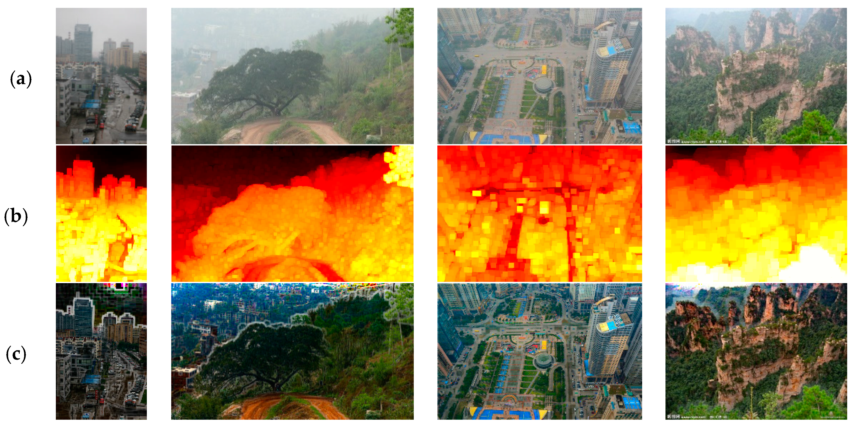
3.3. Multi-Scale Transmission Map Fusion Method

According to the atmospheric scattering model (Equation (2)), with the estimated global atmospheric light, we can directly obtain the rough transmission map $t_{\alpha }$ via DCP (using patch size 15 × 15). However, the DCP is a patch-based procedure in nature, and therefore, the estimated transmission $t_{\alpha }$ may suffer from a poor edge-consistency property.

For experimental demonstration, we choose another four hazy images (see Figure 7a), then obtain the corresponding rough transmission maps $t_{\alpha }$ (see Figure 7b) and the relevant recovered images (see Figure 7c). As we can see, the blocking effects obviously appear in the rough transmission maps $t_{\alpha }$, and therefore, the relevant recovered images are all subjected to severe halo artifacts.

If we reduce the patch size when applying the DCP, the edge-consistency property of the transmission map can be significantly improved. According to this thinking, we can obtain another rough transmission map $t_{\beta }$ using the pixel-level DCP (patch size $1\times 1$). Nevertheless, the estimation accuracy of $t_{\beta }$ is sacrificed inevitably, since the validity of DCP is determined by the information sufficiency contained within the local patch. Consequently, serious negative effects (such as large scale color distortion) appear in the recovered image inevitably.

In Figure 8a, we provide the corresponding transmission maps $t_{\beta }$ for Figure 7a. As we can see, compared with Figure 7b, the edge structure is well maintained in Figure 8a. However, we can also notice that the global color distortion is obvious in the relevant recovered images (see Figure 8c).

Consequently, it is impossible to keep the edge-consistency of the transmission map if we merely adjust the patch size of DCP. Although many transmission map refinement methods (such as the soft matting technique and the filtering-based methods) have been proposed, these methods are either time consuming or lacking in stability [11].

Inspired by [34], we propose a fusion-based global transmission refinement method to overcome this problem. The main concept behind the proposed fusion-based technique is to preserve only the positive features of the two transmission maps ($t_{\alpha }$ and $t_{\beta }$) and therefore improving the edge structure of the transmission map.

By adopting the image pyramid model [35], we decompose the transmission $t_{\alpha }$ into low frequency component $L_{\alpha }^0$ and the high frequency component $\left\{L_{\alpha }^i,i\in \left[1,M\right]\right\}$. Similarly, the transmission $t_{\beta }$ is decomposed into low frequency component $L_{\beta }^0$ and the high frequency component $\left\{L_{\beta }^i,i\in \left[1,M\right]\right\}$. Then, considering that the pyramid model $\left\{L_{\alpha }^i,i\in \left[0,M\right]\right\}$ contains extensive accuracy low frequency component and the pyramid model $\left\{L_{\beta }^i,i\in \left[0,M\right]\right\}$ consists of substantial accuracy high frequency component, the fusion strategy should be designed to support these important features; thus, the bottom level of $\left\{L_{\alpha }^i,i\in \left[0,M\right]\right\}$ should has the highest fusion weight, and the fusion weight should decrease along with the increased level index. Accordingly, the corresponding fusion weight for $\left\{L_{\beta }^i,i\in \left[0,M\right]\right\}$ should be set oppositely. Therefore, we create the adaptive multi-scale transmission fusion method as:

$$\{\begin{array}{l}{L}_i^{fusion}=\left(1-{\gamma }_i\right)\cdot L_{\alpha }^i+{\gamma }_i\cdot L_{\beta }^i,0\le i\le M\\ {\gamma }_i=1-2∕\left(1+exp\left(\frac{i}{M}\right)\right),0\le i\le M\end{array}$$

(10)

where $i$ is the level index of the transmission pyramid model, $\left\{L_i^{fusion},i\in \left[0,M\right]\right\}$ is the obtained transmission pyramid model after fusion, ${\gamma }_i$ is the corresponding adaptive fusion scale for each level, and we set $M$ as 11 after repeated testing.

Now that we have the transmission pyramid model $\left\{L_i^{fusion},i\in \left[0,M\right]\right\}$ and we can generate the final transmission $t^{fusion}$ by reconstructing the $\left\{L_i^{fusion},i\in \left[0,M\right]\right\}$, that is:

$$t^{fusion}=rec\left(L_i^{fusion},i\in \left[0,M\right]\right)$$

(11)

where $rec(\cdot )$ is the reconstruction function. By means of this fusion method, the edge structure can be well preserved in the obtained transmission $t^{fusion}$.

Figure 9 provides two hazy images, the corresponding transmission maps $t^{fusion}$ and the relevant recovered images. From Figure 9, we can notice that, the blocking artifacts are effectively eliminated in the transmission maps $t^{fusion}$, and the recovered images contain relatively few halo artifacts (except for the sky region). However, the sky regions are obviously over-enhanced due to the inherent limitations of DCP, as previously mentioned. In addition, the visual quality of the recovered image is limited, this may be caused by the extensive texture details that are introduced into the $t^{fusion}$ via the fusion procedure.

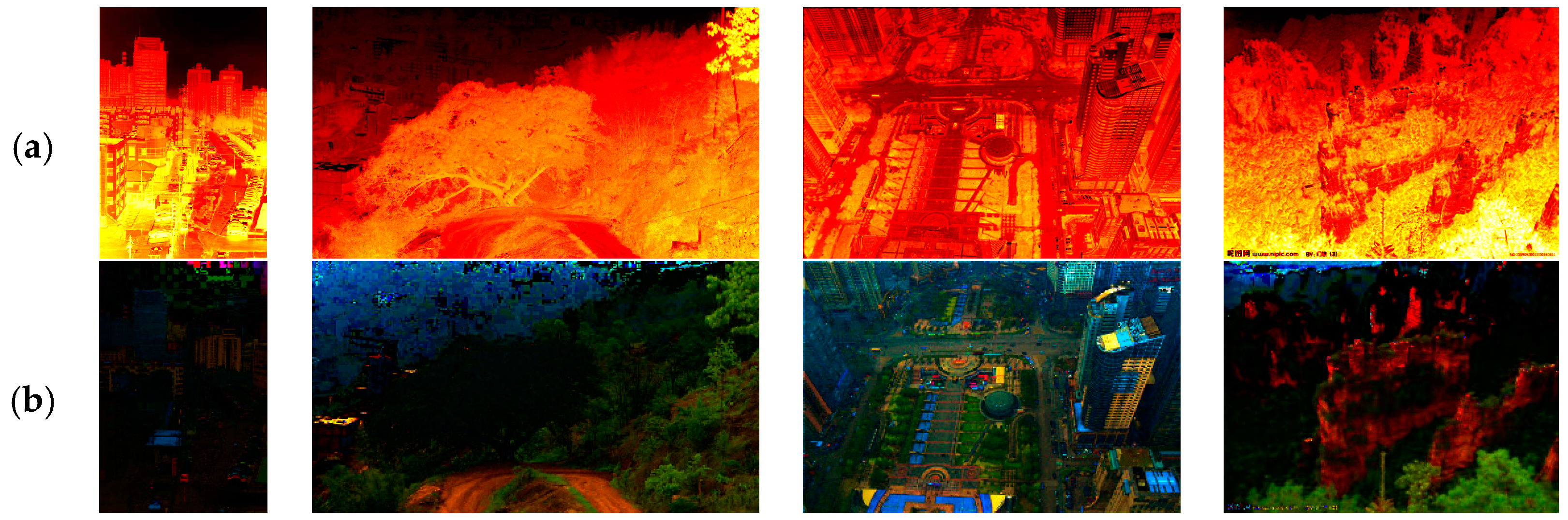
3.4. The Adaptive Sky Region Transmission Correction Method

To correct the transmission within the sky region ${\Delta }_{sky}$ (note that, if no sky region is found via Equation (9), this procedure will be skipped), we design an adaptive correction method based on the following consideration: the brightness of sky region is proportional to the haze density; thus, the magnitude of over-estimation is approximately proportional to the scene feature value $S\left(x,y\right)$. Consequently, the relevant correction magnitude should be adjusted adaptively. Thus, we have:

$$t_{fusion}^{\prime }\left(x,y\right)=min\left(max\left(\frac{S\left(x,y\right)}{mean\left(S\right)},1\right)\cdot max\left(t^{fusion}\left(x,y\right),t_0\right),1\right),\left(x,y\right)\in {\Delta }_{\mathrm{sky}}$$

(12)

where $t_0=0.1$ is the lower boundary of transmission according to [15]. We denote the corrected transmission as $t_{fusion}^{\prime }$.

In Figure 10, we demonstrate the corrected transmission maps $t_{fusion}^{\prime }$ and the corresponding recovered images for Figure 9. It can be noticed that the proposed method can effectively correct the transmission within the sky region and therefore avoid the over-enhancement.

3.5. The Transmission Map Refinement via GTV

The transmission map $t_{fusion}^{\prime }$needs to be further refined because two problems still remain: (1) extensive texture details are still contained in $t_{fusion}^{\prime }$, which may reduce the visual quality of the recovered image; (2) due to the segmentation-blindness of GMM and the scene-based sky region transmission correction method, the edge structure between the sky region and the adjacent areas cannot be well preserved. Thus, we adopt the GTV model [11] to further refine the transmission map $t_{fusion}^{\prime }$, and this procedure can be expressed as:

$$t_{final}=\frac{{\alpha }_1}{2}\cdot {\Vert t_{final}-t_{fusion}^{\prime }\Vert }_2^2+\frac{{\alpha }_2}{2}\cdot \left(W\right)\cdot {\Vert \nabla t_{final}\Vert }_2^2+\frac{{\alpha }_3}{2}\cdot \left(1-W\right)\cdot {\Vert \nabla t_{final}-\nabla G\Vert }_2^2$$

(13)

where $t_{final}$ is the refined transmission map, $W$ is the weight function and $G$ is the guidance image, which is defined as $t_{fusion}^{\prime }$. According to [11], Equation (13) can be expressed and processed using an iteration form, and we have ${\alpha }_1=1.073$, ${\alpha }_2=0.801$and ${\alpha }_3=1.697$ as the regularization parameters for the approximation term, the smoothing term and the edge-preserving term, respectively.

In Figure 11, we show the refined transmission map $t_{final}$ for Figure 9. Through comparing with $t_{fusion}^{\prime }$ (see Figure 10), we can notice that the excessive texture details can be significantly eliminated, and the edge structure between the sky region and the adjacent areas is well refined.

Finally, according to Equation (2), we can directly obtain the scene albedo $\mathsf{\rho }\left(x,y\right)$, since all of the unknown coefficients are determined, including the atmospheric light $L_{\infty }$ and the transmission map $t_{final}$. Then, the image can be recovered as $J\left(x,y\right)=L_{\infty }\cdot \mathsf{\rho }\left(x,y\right)$.

In Figure 12, we provide the images that are recovered using the refined transmission map $t_{final}$. It can be noticed that our method can unveil most of the details, recover vivid color information, with relatively few halo artifacts.

4. Experimental Results

4.1. Transmission Estimation Comparison

In this paper, we present a multi-scale fusion-based strategy, as well as an adaptive sky region transmission correction method to obtain the transmission map and introduce the GTV model to further refine the transmission map. However, to our best knowledge, many transmission estimation methods have been proposed and have made significant progress. In order to verify the advantages of our method, we conduct the experimental comparison with several state-of-the-art methods, including [12,21,26]. We choose two challenging hazy images (a dense haze image without sky region (Figure 13a) and a hazy image with sky region (Figure 13f) for the experimental comparison. The relevant comparison results are provided in Figure 13b–e and Figure 13g–j. As we can see from Figure 13, the transmission maps that are estimated using our method are more consistent with our intuition than those of [12,26] and are comparable to those of [21].

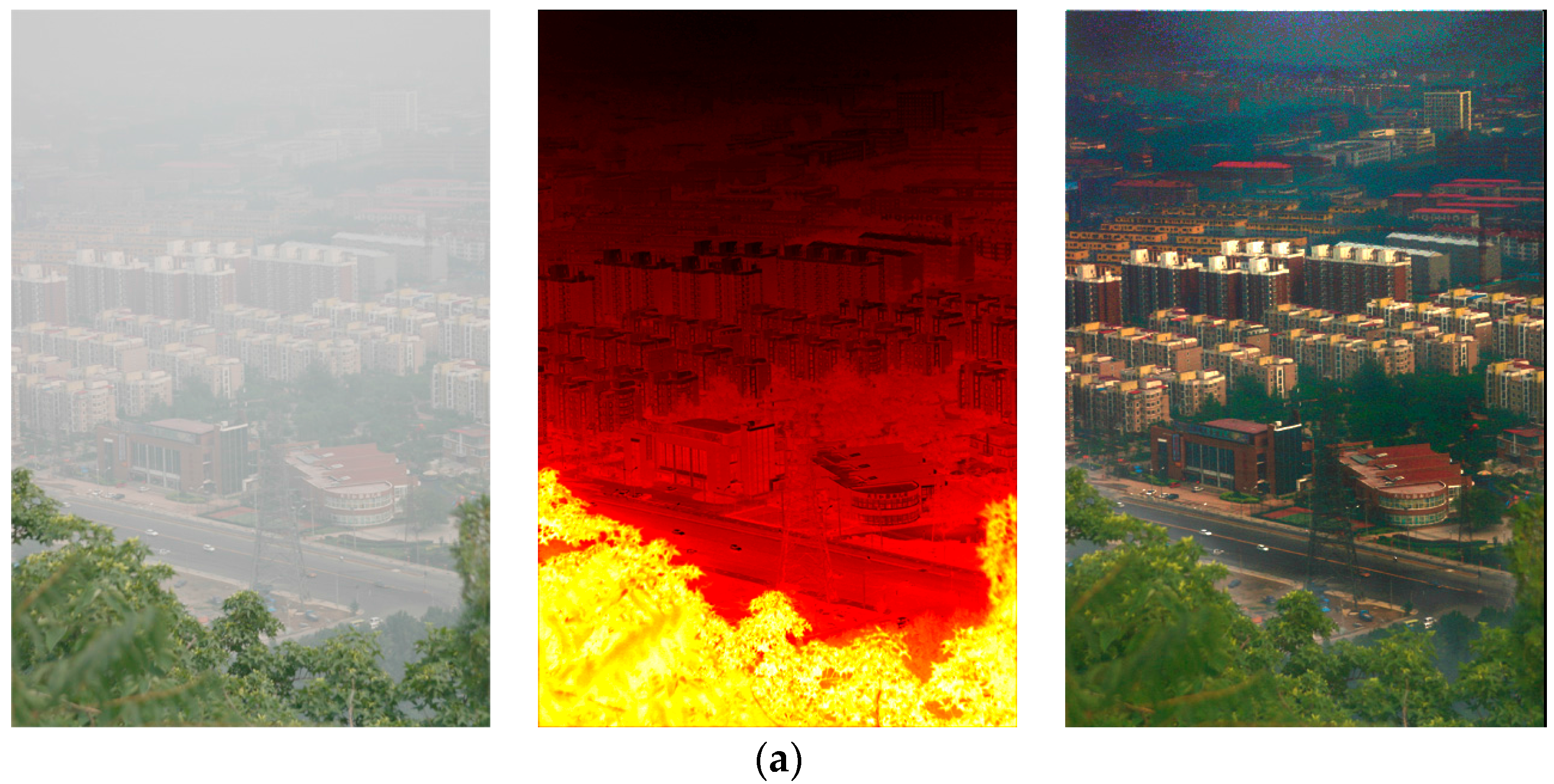
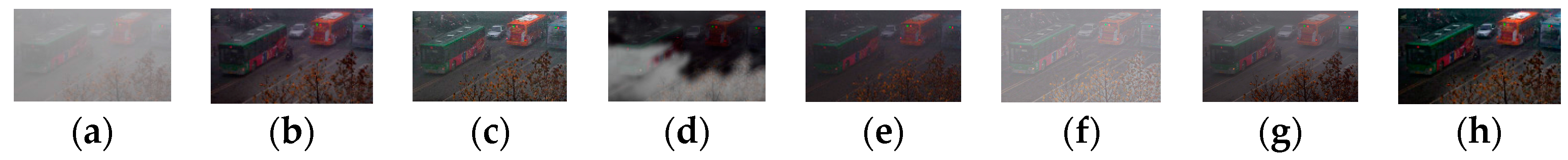
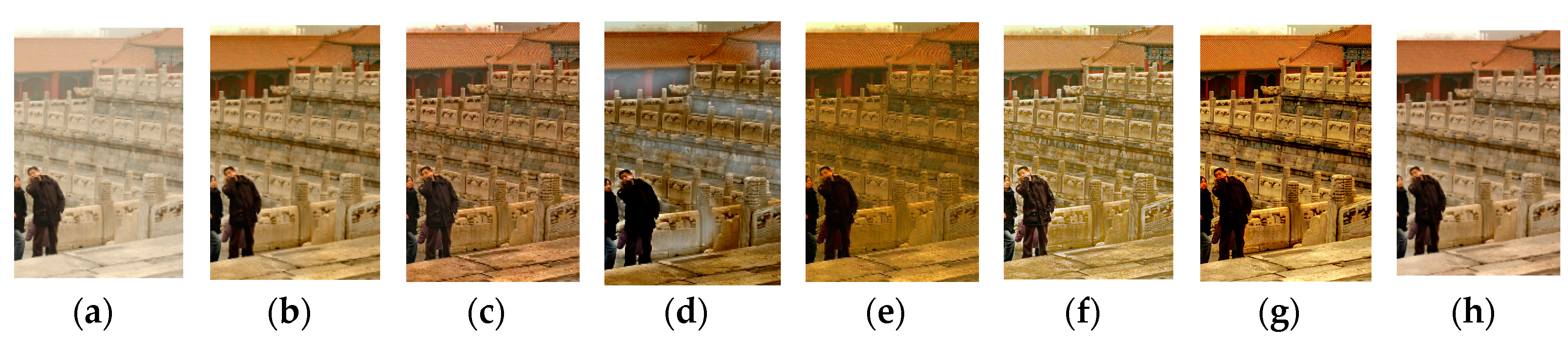
4.2. Qualitative Comparison

To verify the robustness and effectiveness of our method, we test it on various types of challenging hazy images (including both the synthetic image and the real-world image) and conduct qualitative and quantitative comparisons with several state-of-the-art dehazing methods, such as those by He et al. [7], Meng et al. [9], Ancuti et al. [36], Yu et al. [25], Tarel et al. [10] and Choi et al. [17]. All of the methods are implemented in the MATLAB R2014a environment on an Intel Core i5 2.6-GHz PC with 8 GB RAM. The relevant parameters used in the proposed method are demonstrated in Section 3. For fair comparison, we set the parameters used in the other six comparison methods according to [7,9,10,17,25,36].

We compare our method with several state-of-the-art methods on four challenging hazy images, including a synthetic misty image (Figure 14a), a real-world dense haze image (Figure 15a), a real-world hazy image with a large sky region (Figure 16a) and a real-world hazy image with large white/gray regions (Figure 17a). In Figure 14, Figure 15, Figure 16 and Figure 17, The original hazy images are displayed in Column (a); in Columns (b)–(g), from left to right, we demonstrate the dehazing results correspond to He et al.’s [7], Meng et al.’s [9], Ancuti et al.’s [36], Yu et al.’s [25], Tarel et al.’s [10] and Choi et al.’s method [17] and our method, respectively.

Figure 14b, Figure 15b, Figure 16b and Figure 17b show the dehazing results of He et al.’s method [7]. As can be seen, He et al.’s method can generate fine results without halo artifacts, especially when the hazy images do not contain the object whose brightness is similar to the air light (see Figure 14b and Figure 15b). However, owing to the inherent problem of DCP as we discussed, the estimated transmission is thus not reliable enough in some cases. Therefore, the over-enhancement appears within the sky region in Figure 16b, and slightly global color distortion can be found in Figure 17b.

Meng et al.’s method [9] improves the behavior of DCP by adding a boundary constraint, thus the recovered color is more vivid compared with those of He et al.’s method (see Figure 14c and Figure 15c, and compare with Figure 14b and Figure 15b, respectively). Nevertheless, the ambiguity between the image color and haze still cannot be tackled fundamentally; thus, the sky region in Figure 16c is severely over-enhanced, and Figure 17c is subjected to the global color distortion.

In Figure 14d, Figure 15d, Figure 16d and Figure 17d, we provide the dehazing results of Ancuti et al.’s method [36]. As we can see from Figure 15d, the method is not reliable when the hazy images are dark and haze is dense. This is because the performance of [36] is determined by the accuracy of weight maps and therefore may fail when severe dark aspects of the preprocessed image dominate. In addition, haze residual can be found in Figure 14d, as well as Figure 17d.

Yu et al.’s method [25] is another improvement of He et al.’s method [7], and the corresponding dehazing results are demonstrated in Figure 14e, Figure 15e, Figure 16e and Figure 17e. We can notice that this method cannot well handle dense haze image (see Figure 15e); both Figure 14e and Figure 16e are dim and suffer from color distortion; especially, Figure 17e is subjected to serious global color distortion.

The dehazing results of Tarel et al.’s method [10] are shown in Figure 14f, Figure 15f, Figure 16f and Figure 17f. In Figure 16f, most haze is removed, and the scene objects are well unveiled. However, as shown in Figure 15f, Tarel et al.’s method is unable to process the dense hazy image. This is because Tarel et al.’s method utilizes a geometric criterion to decide whether the observed white belongs to the haze or the scene object; thus, it is unreliable under a dense haze condition. Moreover, as previously mentioned, halo artifacts appear inevitably around the depth discontinuities (see Figure 14f and Figure 17f) due to the poor performance of the median filter involved.

In Figure 14g, Figure 15g, Figure 16g and Figure 17g, we provide the dehazing results of Choi et al.’s method [17], which is designed based on a multi-scale fusion strategy. Although this method achieves visually compelling results for Figure 14 and Figure 16, it may be unreliable for some particular case since the image degradation mechanism is not taken into account. As we can see, haze remains significant in Figure 15g, and the global color distortion is severe in Figure 17g.

In contrast, our method can remove most of the haze and well unveil the scene details, maintain the overall color fidelity, significantly eliminate the over-enhancement, with relatively few halo artifacts.

4.3. Quantitative Comparison

In order to quantitatively evaluate and rank the state-of-the-art methods and ours with respect to the structure preserving, visibility enhancement and dehazing effect, we adopt four extensively employed indicators, including the structural similarity (SSIM), the percentage of new visible edges $e$, the contrast restoration quality $\overline{r}$ and the fog-aware density evaluator (FADE). According to [37], the indicator SSIM assesses the structural information preserving ability for a dehazing methods. The indicators $e$ and $\overline{r}$ are proposed by [38], in which the indicator $e$ measures the ratio of edges that are newly visible after restoration, and indicator $\overline{r}$ verifies the average visibility enhancement obtained via restoration. The indicator FADE is proposed by [17], which is an assessment of haze removal ability.

We compute these four indicators (SSIM, $e$, $\overline{r}$ and FADE) on the dehazing results of Figure 14, Figure 15, Figure 16 and Figure 17 and list the corresponding results in

Table 1. Comparison of structural similarity (SSIM) for the dehazing results obtained via different methods.

SSIM	He et al.’s [7]	Meng et al.’s [9]	Ancuti et al.’s [36]	Yu et al.’s [25]	Tarel et al.’s [10]	Choi et al.’s [17]	Ours
Figure 14	0.7283	0.3502	0.4503	0.3109	0.3097	0.6123	0.7694
Figure 15	0.5365	0.6203	0.5284	0.5686	0.7307	0.6993	0.3625
Figure 16	0.7491	0.6986	0.3744	0.4900	0.6768	0.7963	0.7638
Figure 17	0.8220	0.7778	0.2211	0.7296	0.8580	0.6413	0.8801

,

Table 2. Comparison of $\overline{r}$ for the dehazing results obtained via different methods.

$\overline{\mathit{r}}$	He et al.’s [7]	Meng et al.’s [9]	Ancuti et al.’s [36]	Yu et al.’s [25]	Tarel et al.’s [10]	Choi et al.’s [17]	Ours
Figure 14	1.6311	4.5341	3.3588	3.4462	3.8793	1.9113	3.9868
Figure 15	3.7015	4.2383	2.9231	2.0669	2.8428	2.2243	5.2784
Figure 16	1.7584	2.7013	1.9429	1.2296	1.8631	1.4586	2.8840
Figure 17	1.5584	1.7493	2.2455	1.4611	1.5466	1.9429	1.6909

,

Table 3. Comparison of e for the dehazing results obtained via different methods.

e	He et al.’s [7]	Meng et al.’s [9]	Ancuti et al.’s [36]	Yu et al.’s [25]	Tarel et al.’s [10]	Choi et al.’s [17]	Ours
Figure 14	2.3328	1.8269	1.4599	2.4607	2.3789	2.4253	2.5318
Figure 15	53.0796	50.0129	20.0974	35.5132	28.6893	20.3140	53.3612
Figure 16	0.0454	0.3872	0.0046	0.1907	0.5697	0.0850	0.2417
Figure 17	0.3377	0.4775	0.3751	0.6067	0.2177	0.3825	0.4171

and

Table 4. Comparison of fog-aware density evaluator (FADE) for the dehazing results obtained via different methods.

FADE	He et al.’s [7]	Meng et al.’s [9]	Ancuti et al.’s [36]	Yu et al.’s [25]	Tarel et al.’s [10]	Choi et al.’s [17]	Ours
Figure 14	0.3437	0.3589	0.4964	0.2763	0.3158	0.2651	0.2299
Figure 15	0.7070	0.7728	1.2817	0.9385	1.7907	1.2396	0.3767
Figure 16	0.3113	0.2887	0.4049	0.2802	0.4291	0.4792	0.2468
Figure 17	0.2411	0.2190	0.2203	0.1861	0.4108	0.2584	0.2057

, respectively. In addition, we give the time consumption comparison with the five state-of-the-art methods in

Table 5. Comparison of time consumption for the dehazing results obtained via different methods.

Time Consumption	He et al.’s [7]	Meng et al.’s [9]	Ancuti et al.’s [36]	Yu et al.’s [25]	Tarel et al.’s [10]	Choi et al.’s [17]	Ours
Figure 14	1.36	4.02	2.23	1.29	7.60	18.50	0.88
Figure 15	0.94	5.16	2.48	0.82	19.00	24.91	0.79
Figure 16	0.84	2.18	1.69	0.69	1.55	7.13	0.81
Figure 17	0.96	3.33	2.08	0.74	7.38	15.26	0.83

. For comparison convenience, we indicate the top value in bold and the second-highest values in bold and italics.

Generally, higher values of SSIM indicate a better structural information preserving property for a dehazing method; higher values of $e$ and $\overline{r}$ imply better visual improvement after restoration; and lower values of FADE indicate less haze residual (which means a better dehazing ability).

In order to obtain the values of indicator SSIM produced by different methods for Figure 14, Figure 15, Figure 16 and Figure 17, we adopt the ground truth as the reference image for the synthetic hazy image (Figure 14) and utilize the input hazy images as the reference image for real-world hazy images (Figure 15, Figure 16 and Figure 17). The corresponding values of indicator SSIM are listed in Table 1. From Table 1, we can notice that our dehazing results achieve the best SSIM for two hazy images (Figure 14 and Figure 17) and the second best value for Figure 16, which implies the superior structure information preserving ability of the proposed method. Although the SSIM of our result for Figure 15 is relatively low, the result needs to be balanced. As we can see, Tarel et al.’s method and Choi et al.’s method achieve the top and second top value for Figure 15, respectively. However, this may be caused by the haze residual (haze remains obviously in both of their dehazing results and can be verified via the corresponding FADE values in Table 4) since we adopt the input hazy images as the reference image for real-world hazy images. In contrast, our result removes most of the haze and unveils the majority of the scene objects, which can be further verified via the FADE value from Table 4.

As shown in Table 2, our dehazing results achieve the top values for two hazy images (Figure 15 and Figure 16) and the second top value for Figure 14, which verify the robustness and effectiveness of our method for visibility recovering. Despite Meng et al.’s result being higher than ours for Figure 14, we deduce that it may be caused by the noise amplification. This is because our method can restore more visible edges for Figure 14 (see Table 3), and the value of e for Meng et al.’s result is much lower than ours. Besides, the fusion strategy proposed by Ancuti et al. cannot work for Figure 17 (see Figure 17d), and the top value of $\overline{r}$ may be caused by the poor edge-consistency property.

According to Table 3, our results yield the top value for Figure 14 and Figure 15. Although our results only achieve the third best value for Figure 16 and Figure 17, however, the result of $e$ can be increased when artificial edges become visible; for instance, Meng et al.’s results have the second highest value for Figure 16, whereas the most serious over-enhancement appears in the sky region of Figure 16c.

As shown in Table 4, our method outperforms other methods for Figure 14, Figure 15 and Figure 16 and achieves the second best value for Figure 17, and these results are well consistent with our observation of the qualitative comparison. This verifies the advantage of our method with respect to haze removal ability.

The time consumption is another important evaluation factor for a dehazing algorithm. In Table 5, we give the time consumption comparison of the above methods in Figure 14 (616 × 462), Figure 15 (845 × 496), Figure 16 (291 × 345) and Figure 17 (400 × 600). As we can see, Yu et al.’s method [25] is slightly faster than ours. However, it is a trade-off between effectiveness and efficiency in nature, since the results of [25] are inferior to our method in terms of both qualitative quality and quantitative results. Our method is faster than He et al.’s [7,26], Meng et al.’s [9], Ancuti et al.’s [36], Tarel et al.’s [10] and Choi et al.’s [17]. We attribute this advantage of our method to the proposed fusion-based strategy.

5. Discussion and Conclusions

In this paper, we have presented a simple, but effective single image dehazing method aiming at overcoming the inherent limitations of DCP. Benefitting from the scene segmentation based on the haze density feature map, we can effectively detect the sky region, which allows us to improve the accuracy of atmospheric light estimation. Then, the multi-scale transmission map fusion method and the adaptive sky region transmission correction method are proposed to obtain the transmission map with accurate edge structure. The GTV model is adopted to further refine the edge structure between the sky region and the adjacent area and eliminate the extensive texture details contained in the transmission map. Experimental results verified the advantage of our method compared with several state-of-the-art alternatives.

However, our work also shares the common limitation of most model-based single image dehazing methods. That is, the scattering coefficient $\beta$ in the atmospheric scattering model is regarded as a constant, which conflicts with the inhomogeneous atmospheric conditions. In addition, the cluster number in the scene segmentation procedure and the level number in the fusion procedure need to be determined adaptively. We leave these problems for our future research.

References

1. Narasimhan, S.G.; Nayar, S.K. Contrast restoration of weather degraded images. IEEE Trans. Pattern Anal. Mach. Intell. 2003, 25, 713–724. [Google Scholar] [CrossRef]
2. Narasimhan, S.G.; Nayar, S.K. Vision and the atmosphere. Int. J. Comput. Vis. 2002, 48, 233–254. [Google Scholar] [CrossRef]
3. Nayar, S.K.; Narasimhan, S.G. Chromatic framework for vision in bad weather. In Proceedings of the IEEE Conference on Computer Vision and Pattern Recognition, Hilton Head, SC, USA, 13–15 June 2000; pp. 598–605. [Google Scholar]
4. Tan, R.T. Visibility in bad weather from a single image. In Proceedings of the IEEE Conference on Computer Vision and Pattern Recognition, Anchorage, AK, USA, 23–28 June 2008; pp. 1–8. [Google Scholar]
5. Fattal, R. Single image dehazing. ACM Trans Graph. 2008, 27, 1–9. [Google Scholar] [CrossRef]
6. Zhu, Q.; Mai, J.; Shao, L. A fast single image haze removal algorithm using color attenuation prior. IEEE Trans. Image Process. 2015, 24, 3522–3533. [Google Scholar] [PubMed]
7. He, K.; Sun, J.; Tang, X. Single image haze removal using dark channel prior. IEEE Trans. Pattern Anal. Mach. Intell. 2009, 33, 2341–2353. [Google Scholar]
8. Ju, M.Y.; Gu, Z.F.; Zhang, D.Y. Single image haze removal based on the improved atmospheric scattering model. Neurocomputing 2017. [Google Scholar] [CrossRef]
9. Meng, G.; Wang, Y.; Duan, J.; Xiang, S. Efficient image dehazing with boundary constraint and contextual regularization. In Proceedings of the IEEE Conference on Computer Vision, Sydney, Australia, 1–8 December 2013; pp. 617–624. [Google Scholar]
10. Tarel, J.P.; Hautiere, N. Fast visibility restoration from a single color or gray level image. In Proceedings of the IEEE Conference on Computer Vision, Kyoto, Japan, 29–30 September 2009; pp. 2201–2208. [Google Scholar]
11. Ju, M.; Zhang, D.; Wang, X. Single image dehazing via an improved atmospheric scattering model. Vis. Comput. 2016, 1–13. [Google Scholar] [CrossRef]
12. Xiao, C.; Gan, J. Fast image dehazing using guided joint bilateral filter. Vis. Comput. 2012, 28, 713–721. [Google Scholar] [CrossRef]
13. Xie, B.; Guo, F.; Cai, Z. Improved single image dehazing using dark channel prior and multi-scale retinex. In Proceedings of the IEEE Conference on Intelligent System Design and Engineering Application, Changsha, China, 13–14 October 2010; pp. 848–851. [Google Scholar]
14. Yu, J.; Xiao, C.; Li, D. Physics-based fast single image fog removal. Acta Autom. Sin. 2010, 37, 1048–1052. [Google Scholar]
15. Zhang, D.Y.; Ju, M.Y.; Wang, X.M. A fast image daze removal algorithm using dark channel prior. Chin. J. Electron. 2015, 43, 1437–1443. [Google Scholar]
16. Ju, M.Y.; Zhang, D.Y.; Ji, Y.T. Image haze removal algorithm based on haze thickness estimation. Acta Autom. Sin. 2016, 42, 1367–1379. [Google Scholar]
17. Choi, L.K.; You, J.; Bovik, A.C. Referenceless prediction of perceptual fog density and perceptual image defogging. IEEE Trans. Image Process. 2015, 24, 3888–3901. [Google Scholar] [CrossRef] [PubMed]
18. Wang, J.B.; He, N.; Zhang, L.L.; Lu, K. Single image dehazing with a physical model and dark channel prior. Neurocomputing 2015, 149, 718–728. [Google Scholar] [CrossRef]
19. Yeh, C.H.; Kang, L.W.; Lee, M.S; Lin, C.Y. Haze effect removal from image via haze density estimation in optical model. Opt. Express 2013, 21, 27127–27141. [Google Scholar] [CrossRef] [PubMed]
20. Gu, Z.F.; Ju, M.Y.; Zhang, D.Y. A single image dehazing method using average saturation prior. Math. Probl. Eng. 2017, 2017, 1–17. [Google Scholar] [CrossRef]
21. Li, B.; Wang, S.; Zheng, J.; Zheng, L. Single image haze removal using content-adaptive dark channel and post enhancement. IET Comput. Vis. 2014, 8, 131–140. [Google Scholar] [CrossRef]
22. Galdran, A.; Vazquez-Corral, J.; Pardo, D.; Bertalmio, M. Fusion-based variational image dehazing. IEEE Signal Process. Lett. 2017, 24, 151–155. [Google Scholar] [CrossRef]
23. Galdran, A.; Vazquez-Corral, J.; Pardo, D.; Bertalmío, M. A variational framework for single image dehazing. In Presented at the Proceedings of the European Conference on Computer Vision, Heidelberg, Germany, 20 March 2014; pp. 259–270. [Google Scholar]
24. Yoon, I.; Jeong, S.; Jeong, J.; Seo, D.; Paik, J. Wavelength-Adaptive Dehazing Using Histogram Merging-Based Classification for UAV Images. Sensors 2015, 15, 6633–6651. [Google Scholar] [CrossRef] [PubMed]
25. Yu, T.; Riaz, I.; Piao, J.; Shin, H. Real-time single image dehazing using block-to-pixel interpolation and adaptive dark channel prior. IET Image Process. 2015, 9, 725–734. [Google Scholar] [CrossRef]
26. He, K.M.; Sun, J.; Tang, X.O. Guided image filtering. IEEE Trans. Pattern Anal. Mach. Intell. 2013, 35, 1397–1409. [Google Scholar] [CrossRef] [PubMed]
27. Shi, Z.; Long, J.; Tang, W.; Zhang, C. Single image dehazing in inhomogeneous atmosphere. Optik 2014, 125, 3868–3875. [Google Scholar] [CrossRef]
28. Li, Y.; Miao, Q.; Song, J.; Quan, Y.; Li, W. Single image haze removal based on haze physical characteristics and adaptive sky region detection. Neurocomputing 2015, 182, 221–234. [Google Scholar] [CrossRef]
29. Reynolds, D.A.; Quatieri, T.F.; Dunn, R.B. Speaker verification using adapted Gaussian mixture models. Digit. Signal Process. 2000, 10, 19–41. [Google Scholar] [CrossRef]
30. Yu, F.; Qing, C.M.; Xu, X.M.; Cai, B.L. Image and video dehazing using view-based cluster segmentation. In Proceedings of the IEEE Conference on Visual Communications and Image Processing, Chengdu, China, 27–30 November 2016; pp. 1–4. [Google Scholar]
31. Haralick, R.M.; Sternberg, S.R.; Zhuang, X. Image analysis using mathematical morphology. IEEE Trans. Pattern Anal. Mach. Intell. 1987, 9, 532–550. [Google Scholar] [CrossRef] [PubMed]
32. Sulami, M.; Glatzer, I.; Fattal, R.; Werman, M. Automatic recovery of the atmospheric light in hazy images. In Proceedings of the IEEE Conference on Computational Photography, Santa Clara, CA, USA, 2–4 May 2014; pp. 1–11. [Google Scholar]
33. Shwartz, S.; Namer, E.; Schechner, Y.Y. Blind haze separation. In Proceedings of the IEEE Computer Society Conference on Computer Vision and Pattern Recognition, Washington, DC, USA, 17–22 June 2006; pp. 1984–1991. [Google Scholar]
34. Wang, S.; Li, B.; Zheng, J. Parameter-adaptive nighttime image enhancement with multi-scale decomposition. IET Comput. Vis. 2016, 10, 425–432. [Google Scholar] [CrossRef]
35. Burt, P.J.; Adelson, E.H. The Laplacian pyramid as a compact image code. IEEE Trans. Commun. 1983, 31, 532–540. [Google Scholar] [CrossRef]
36. Ancuti, C.O.; Ancuti, C. Single image dehazing by multi-scale fusion. IEEE Trans. Image Process. 2013, 22, 3271–3282. [Google Scholar] [CrossRef] [PubMed]
37. Wang, Z.; Bovik, A.C.; Sheikh, H.R.; Simoncelli, E.P. Image quality assessment: from error visibility to structural similarity. IEEE Trans. Image Process. 2004, 13, 600–612. [Google Scholar] [CrossRef] [PubMed]
38. Hautière, N.; Tarel, J.P.; Aubert, D.; Dumont, E. Blind contrast enhancement assessment by gradient ratioing at visible edges. Image Anal. Stereol. 2008, 27, 87–95. [Google Scholar] [CrossRef]
Figure 1. Overview of our method. From the input hazy image, we first detect the sky region based on the haze density feature map and scene segmentation technique. Then, we apply three key steps, including the improved global atmospheric light estimation, the multi-scale transmission map fusion and the adaptive sky region transmission correction. Next, we introduce the guided total variation (GTV) to further refine the transmission map and recover image via the atmospheric scattering model.
Information 08 00057 g001
Figure 2. Hazy images and the corresponding haze density feature maps. (a): hazy images. (b): the corresponding haze density feature mapsobtained via Equation (4).
Information 08 00057 g002
Figure 3. The relevant scene segmentation results for Figure 2. We segment the hazy image into three scenes and mark them using red, green and blue, respectively. (a): The scene segmentation result for Figure 2a (left). (b) The scene segmentation result for Figure 2a (right).
Information 08 00057 g003
Figure 4. Accuracy rate of sky region detection using different sky region feature lower boundary values.
Information 08 00057 g004
Figure 5. The detected sky region (marked as white area) for Figure 2 using our method. (a): The detected sky region (marked as white area) for Figure 2a (left). (b) The detected sky region (marked as white area) for Figure 2a (right).
Information 08 00057 g005
Figure 6. A challenging hazy image for the atmospheric light locating comparison and the recovery effect comparison of different atmospheric light estimation results. (a) Atmospheric light locating comparison, the results of [6,7,33] and ours are depicted in boxes with different colors. (be) The recovery effect comparison; the images are recovered using different atmospheric light estimation results that are obtained via [6,7,33] and ours, respectively.
Information 08 00057 g006
Figure 7. Hazy images, the corresponding rough transmission maps t α and the relevant recovered images. (a): hazy images. (b): the corresponding rough transmission maps t α . (c): the relevant recovered images.
Information 08 00057 g007
Figure 8. The transmission maps t β estimated using pixel-level DCP and the relevant restored images for Figure 7, top. (a): the transmission maps t β . (b): the relevant restored images.
Information 08 00057 g008
Figure 9. From left to right: two challenging haze images, the corresponding transmission maps t f u s i o n and the relevant recovered images. (a) Hazy image with small sky region, the corresponding transmission map t f u s i o n , and the relevant recovered image. (b) Hazy image with large sky region, the corresponding transmission map t f u s i o n , and the relevant recovered image.
Information 08 00057 g009aInformation 08 00057 g009b
Figure 10. The corrected transmission maps t f u s i o n for Figure 9, and the corresponding recovered images. (a) The corrected transmission map t f u s i o n for the hazy image of Figure 9a, and the corresponding recovered image. (b) The corrected transmission map t f u s i o n for the hazy image of Figure 9b, and the corresponding recovered image.
Information 08 00057 g010
Figure 11. The refined transmission maps t f i n a l for Figure 9 via the GTV model. Left: The refined transmission map t f i n a l for the hazy image of Figure 9a. Right: The refined transmission map t f i n a l for the hazy image of Figure 9b.
Information 08 00057 g011
Figure 12. The corresponding images that are recovered via the refined transmission map t f i n a l . (a): The recovered image for the hazy image of Figure 9a. (b): The recovered image for the hazy image of Figure 9b.
Information 08 00057 g012
Figure 13. Comparison of the transmission maps that are estimated via [12,21,26] and our method. (a) A dense haze image without sky region. (be) From left to right; top: the transmission maps that are estimated via [12,21,26] and our method, respectively; bottom: the corresponding recovered images. (f) A hazy image with sky region. (gj) From left to right; top: the transmission maps that are estimated via [12,21,26] and our method, respectively; bottom: the corresponding recovered images.
Information 08 00057 g013
Figure 14. Qualitative comparison on synthetic misty image. (a) Synthetic misty image. (b) He et al.’s result. (c) Meng et al.’s result. (d) Ancuti et al.’s result. (e) Yu et al.’s result. (f) Tarel et al.’s result. (g) Choi et al.’s result. (h) Our result.
Information 08 00057 g014
Figure 15. Qualitative comparison on dense haze image. (a) Dense haze image. (b) He et al.’s result. (c) Meng et al.’s result. (d) Ancuti et al.’s result. (e) Yu et al.’s result. (f) Tarel et al.’s result. (g) Choi et al.’s result. (h) Our result.
Information 08 00057 g015
Figure 16. Qualitative comparison on hazy image with large sky region. (a) Hazy image with large sky region. (b) He et al.’s result. (c) Meng et al.’s result. (d) Ancuti et al.’s result. (e) Yu et al.’s result. (f) Tarel et al.’s result. (g) Choi et al.’s result. (h) Our result.
Information 08 00057 g016
Figure 17. Qualitative comparison on hazy image with large white/gray regions. (a) Hazy image with large white/gray regions. (b) He et al.’s result. (c) Meng et al.’s result. (d) Ancuti et al.’s result. (e) Yu et al.’s result. (f) Tarel et al.’s result. (g) Choi et al.’s result. (h) Our result.
Information 08 00057 g017