Article

Identifying High Quality Document–Summary Pairs through Text Matching

Intelligence Computing Research Center, Harbin Institute of Technology Shenzhen Graduate School, Shenzhen 518055, China
*
Author to whom correspondence should be addressed.
Information 2017, 8(2), 64; https://doi.org/10.3390/info8020064
Submission received: 28 March 2017 / Revised: 3 June 2017 / Accepted: 7 June 2017 / Published: 12 June 2017
(This article belongs to the Special Issue Text Mining Applications and Theory)

Abstract

:
Text summarization namely, automatically generating a short summary of a given document, is a difficult task in natural language processing. Nowadays, deep learning as a new technique has gradually been deployed for text summarization, but there is still a lack of large-scale high quality datasets for this technique. In this paper, we proposed a novel deep learning method to identify high quality document–summary pairs for building a large-scale pairs dataset. Concretely, a long short-term memory (LSTM)-based model was designed to measure the quality of document–summary pairs. In order to leverage information across all parts of each document, we further proposed an improved LSTM-based model by removing the forget gate in the LSTM unit. Experiments conducted on the training set and the test set built upon Sina Weibo (a Chinese microblog website similar to Twitter) showed that the LSTM-based models significantly outperformed baseline models with regard to the area under receiver operating characteristic curve (AUC) value.

1. Introduction

In the era of the Internet, we as humans share our experiences or transfer information between each other through multimedia processes, such as instant messaging, question-answering communities, and microblogs. Many of us can receive hundreds or thousands of messages posted by official news agencies, professional commentators, or people we pay attention to daily, most of which offer valuable information to us. It is a heavy load to process all this information, so it becomes more important to examine how to capture the brief ideas that the messages convey.
Automatic text summarization is the task of generating short summaries from the given long documents [1]. A summary includes the main idea of a given document, which is essentially what this document aims to express. As an example, a weibo is a microblog message, from one of the most popular Chinese microblog websites, Sina Weibo (http://www.weibo.com) (shown in Table 1). A weibo message is composed of a document and its summary. The document can have up to 140 Chinese characters while the summary written by the publisher usually only contains approximately 10–20 characters. By scanning the summary, we can rapidly identify whether a message is interesting for us and whether we need to read the full document word by word. Therefore, a good summarization system is necessary for us, as we may face massive amounts of information from different sources.
Automatic text summarization has been studied for years from extractive summarization to abstractive summarization [2]. In recent years, the task has been boosted by the development of deep learning algorithms and the explosive growth of data [3], especially for abstractive summarization. Large-scale high quality document–summary pairs are a precondition of high quality automatic text summarization. Summaries of documents are usually manually written, which is too expensive. An alternative way is to utilize existing raw data from the web to help us to build large document–summary training corpora (i.e., Weibo offers a large number of document–summary pairs posted by human beings). Hu et al. built their corpus by crawling raw pairs data from Weibo and filtering with the help of hundreds of heuristic rules [4]. However, building and validating these rules for filtering are also a time-consuming process.
In this paper, we proposed a novel method to extract high quality document–summary pairs. Concretely, we firstly trained a text matching model on a labeled corpus of document–summary pairs with matching degrees, then applied the model on unlabeled document–summary pairs to check their matching degree. Following this, the document–summary pairs with a high matching degree were selected. We needed almost no additional rules from developers and also complex feature engineering. The text matching model was based on a deep neural network, which had been successful in learning distributional representations of the original text and capturing feature information efficiently through well-built network architectures. In typical natural language processing tasks such as textual entailment [5], machine translation [6], question–answer matching [7,8], deep Convolutional Neural Networks (CNN), and deep Recurrent Neural Networks (RNN) and their variants, such as Long Short-Term Memory (LSTM) [9,10] and Gate Recurrent Unit (GRU) [11,12], were the models favored by most studies and the architectures built upon them had allowed for constant state-of-the-art results in these tasks. There are two main advantages of the deep learning model. On one hand, deep learning has superior learning abilities than traditional statistical machine learning. On the other hand, we can make full use of the huge amount of crawled text for unsupervised learning so as to learn more representative word–character embeddings.
Another issue we should tackle in this paper is adaptation to the diverse cases in the crawled document–summary pairs. Social media (i.e., Sina Weibo) is an open community in which users from all walks of life can post documents and summaries freely. Hence, there are no strict rules for the users to follow when they summarize their documents. As a result, the types of the crawled summaries cannot be guaranteed to be the same type. For example, one may simply pick out several words or sentences in the posted document when the publisher is not good at summarization or just wants to save time (i.e., Table 2). For pairs of documents and their summarizations in social media, the writing styles change greatly, as shown in Table 2, Table 3 and Table 4. The aim of this paper is to identify high quality document–summary pairs and remove noisy pairs with a trained model that can adapt to more document pair writing styles.
To get models for high quality document–summary pairs identifying, we firstly modified the convolutional architecture(ARC)-I proposed by Hu et al. [5] for matching two sentences, where each text segment (a document or a summary) was encoded into a fixed length vector with semantic correlation of a text pair then being evaluated through adding a multi-layer perceptron (MLP). Secondly, we built a LSTM-based model to improve the ability of learning long range dependencies. Compared with CNN, using RNN with LSTM units was appropriate for sequential inputs such as audio signal and natural language [13]. In the model, each text segment was encoded by LSTM and mean-pooling, which could preserve most information from the start to the end of the text segment. Thirdly, as LSTM still having the issue of information loss, we modified the LSTM unit by removing the forget gate so that the information across the sequence could hardly be refreshed through the network. The intuitions for the modification were mainly two phases: (1) The vanishing of gradients was still inevitable for LSTM when handed long sequences due to its architecture when a great number of documents in the Weibo data set had relatively long text lengths (over 50 words); (2) Some summaries were abstractive conclusions of the original documents, the generations of which needed an overview of the whole documents. As the forget gate played the role of removing duplicate or useless parts of the representation, a neural unit without the forget gate could retain more information from the beginning.
We carried out our experiments on a dataset randomly sampled from a benchmark corpus, the large-scale Chinese short text summarization (LCSTS) dataset [4]. The document–summary pairs in the dataset had been manually tagged as high or low quality with agreed hierarchical scores from several annotators, based on the degree of coherence between a document and its corresponding summary. The high-quality pairs were taken as positive samples while the low quality ones were negative in this paper. The dataset was further divided into training, development, and test sets. We compared the proposed LSTM model and the improved LSTM model with Recall-oriented understudy of gisting evaluation (ROUGE)-based method, supporting vector machines (SVM), latent semantic indexing (LSI), CNN, gated recurrent unit (GRU), and bidirectional LSTM (bi-LSTM). The experiment results showed that the improved LSTM model achieved an optimal area under receiver operating characteristic curve (AUC) value and outperformed the basic LSTM model by 1.16% on the training set and 0.92% on the test set.
The contributions of this paper were: (1) we analyzed the annotated document–summary pairs with five-score levels, and defined the score level for high quality document–summary pairs based on the five-score levels; (2) we proposed an LSTM-based model to identify high quality document–summary pairs which could be used to build a large-scale document–summary pairs dataset; (3) we improved the LSTM-based model to make it more suitable for identifying document–summary pairs.

2. Related Works

2.1. Automatic Text Summarization

The supervised single-document summarization techniques were the focus of this section. There were mainly two categories for automatic text summarization: extractive summarization and abstractive summarization [14,15]. The prior one aimed to identify summary sentences or summary words from a document that was a good description of the bones of the document before placing them in order [16,17,18]. In comparison, the latter one was not constrained by using the original sentences or words in the document and could generate a more abstractive summary [19,20,21]. In the supervised machine learning literature, feature-based methods including using classifiers [22,23], graphic models [19,24,25], and cluster methods [26,27] had played a vital role in the past years. Nowadays, deep learning based methods simplified the process of feature extraction [5,28,29]. By using sequence to sequence learning and generation techniques, deep models could capture the informative parts from the document and generate extractive or abstractive summaries [21,30,31]. The superior learning ability of deep neural networks greatly enhanced the state-of-the-art performance in this research field.
One of the issues for deep learning based methods was the requirement of a large-scale training corpus in order to completely estimate the huge number of parameters in well-built networks. Most of the existing benchmark datasets only contained a relatively small number of training pairs which were not enough for training deep networks. For example, in document understanding conference (DUC) datasets, there were only 567 documents belonging to 59 different topics in total in the DUC-2002 dataset and 624 document–summary pairs in the DUC-2003 dataset [32]. In the Opinosis dataset, there were 51 different topics, with each topic comprising of 50–575 sentences and including four or five gold standard summaries created by a human [19]. In the Text Analysis Conference (TAC) 2011 summarization track dataset, there were only 440 documents belonging to 44 topics, with 10 for each topic [33]. In recent years, many researchers had constructed new datasets in order to satisfy their neural models and achieved some progress in this field of research [4,34,35]. Nevertheless, a normal way for collecting such large-scale datasets was through applying web crawlers [4] or document extractors [34], by which the quality of the data could not be guaranteed. Hence it is necessary to exploit methods for automatically identifying high-quality pairs.

2.2. Text Matching

Text matching was widely applied in natural language processing (i.e., information retrieval, textual entailment, machine translation, and question answering). Generally speaking, literature could be roughly divided into statistical learning and deep learning. The feature vectors for statistical learning were usually extracted through a vector space model (VSM) [36] and its variants (i.e., term frequency–inverse document frequency (TF–IDF), mutual information and other methods), Latent Semantic Indexing (LSI) [37,38] or Latent Dirichlet Allocation (LDA) [39]. In VSM, a text was first transformed into a representation in the vector space, each dimension of which stood for the weight of the corresponding word in the text. The main advantage of VSM was its fast speed in feature extraction and computation, while the main disadvantage was the loss of semantic differences between words, including even synonyms and antonyms. LSI could tackle this issue by constructing a matrix containing each word and each text so that the relations between words and the texts could be formulated, in addition to the relationship between words [37]. By utilizing singular value decomposition (SVD) [40], a text could be represented as the multiplication of three sub-matrices. An improved version of LSI is LDA [39]. LDA introduced a concept of a topic and assumed that a document could be represented as a distribution on topics with a topic being seen as a distribution of words. In many cases, LDA and LSI performed comparatively well, especially in text classification. The above techniques were to generate representations of documents. With these representations (feature vectors), the matching degree for a text pair could be determined by cosine similarity or classifiers such as the Maximum Entropy Classifier and SVM [22].
A main drawback of the statistical learning methods is the omission of word orders, which is very important when understanding a text segment. For example, the sentences “Michael sent the book to Chris.” and “Chris sent the book to Michael.” have seven common words which cannot be distinguished by VSM or LSI, despite the distinct meanings of each sentence. Deep learning methods can address the above issue through the operation of convolution or recurrent units. In the deep learning based models, a text segment is firstly augmented with word/character embeddings. Word embeddings are often pre-trained in an unsupervised way in a large text corpus [41]. It conveys the semantic meaning of the current word through the distributional dimensions and the distance in the distribution space of two vectors stands for the semantic similarity between them. With the word embeddings, semantic features for work can be extracted directly.
Deep learning methods were widely used on text-processing tasks, including sentiment analysis, machine translation, question answering, and textual entailment, in recent studies based on pre-trained word embedding. In a previous study [42], deep CNN was used to extract features from short texts for utterance-level multimodal sentiment analysis. Another study [43] also used a seven-layer deep CNN to tag each word in opinionated sentences as either aspect or non-aspect words with the tag results used to extract aspects opinion mining. In study [5], CNN modeled each word in the sentence into fixed length vectors in a pair and generated a combined vector for similarity evaluation. The study [6] used a encoder decoder model to learn the matching between the source and target sentences in a machine translation, which integrated GRU as the recurrent unit. The study [8] applied a CNN–LSTM model to capture the dependences in a community question answering thread so as to learn question-answer matching. Another study [44] added additional attention information on hidden representations to obtain attentive sentence representation and used the result for answer selection. Another study [10] adopted a deep fusion strategy to model the strong interactions of two sentences based on LSTMs, with experiments demonstrating its efficacy with regards to the question answering matching task and textual entailment task. A previous study [45] developed hybrid models by combining convolutional and recurrent neural networks to process passage answers for the question answering matching task. Study [46] proposed a deep neural network-based method, which employed bi-LSTM to read question title and body, to analyze and quantify the relation between question title and body in community question answering.
Deep learning methods were also used for textual entailment recognition, recently. For example, in [47], word embeddings learnt by deep learning methods were used to train classifiers for textual entailment recognition. A joint Restricted Boltzmann Machines Layer was used to learn a joint representation for textual entailment recognition [48]. LSTM with the word-by-word neural attention mechanism to read two sentences was proposed to reasoning and determine textual entailment in [49]. Deep fusion LSTM model on the strong interaction of text pair was proposed to matching text semantic matching in a recursive matching way, and the model performed excellently on text semantic matching task, including the textual entailment recognition and the question and answer matching [10].
Document–summary pairs identification is partially distinct from other short text matching tasks in that: (1) the given document may contain more than one semantic text segment that can express several ideas, hence it is a document-level text; (2) although the target summary is short, it should cover most parts of the document instead of one or two single points. The characteristics demand that when using the deep learning, the architectures of the basic algorithm may need improvement so as to adapt to the special sample styles. As a result, when conducting noise reduction and building a high-quality training corpus, we also have to take these issues into account.

3. Corpus Construction and Analysis

The Large Scale Chinese Short Text Summarization (LCSTS) corpus released by Hu et al. contained 2,400,591 document–summary pairs crawled automatically from Sina Weibo and 11,772 pairs dataset with quality scores labels [4]. We removed those pairs with a length of the document being too short (length of title less than 5 characters, or length of weibo less than 10 characters) from the labeled dataset in the corpus. Finally, we got 11,675 document–summary pairs. We tagged each document–summary pair as positive or negative according to their quality scores (provided by the corpus). The scores fell into five levels: (1) the provided title we also refer to the original provided summary as the “title” and the document as a “weibo” for easier description cannot be taken as the summary of the document, i.e., the title is non-related or is a comment to the document (Table 3); (2) the title is a partially related to the document, i.e., the title is segment selected from the document (Table 2); (3) the title is related to the document to some extent but it can only covers a half of the document at most, i.e., the title only reflects the first part of the document (Table 4); (4) the title can almost be the summary of the document (Table 5); (5) the title can be a good summary of the document (Table 1). The scores from 1 to 5 are assigned to different levels corresponding to the above descriptions.
The data was annotated by five volunteers. The five volunteers were selected from computer science and technology post graduate students, who have some background in information retrieval and computational linguistics. In the training set, each pair was labeled by only one annotator; in the development set and the test set, each pair was the pair that was labeled by three annotators and had same score.
We commence a deeper analysis of the noisy pairs in the crawled data. In Table 3, although the document discusses the topic of being middle-class, we can see few relations between the document and the title in the text and there are almost no characters in common. The title is a comment after reading the document. It is almost impossible to generate such a title given this document, so it is obviously a bad sample. In Table 2, the title is the first sentence of the document. It is believed that the author of the document randomly typed or copied a sentence to be the title without summarizing the whole document. In Table 4, the title only conveys the first sentence content about the film landing time, but loses the last sentence content about the actor Bruce Willis. Those are noisy samples since the document shows several points but the title only covers one, which may cause an incomplete learning of the model.
For dataset building, we extracted the pairs with scores of four or five as positive samples and the rest as negative samples. It was considered that the summary must cover most of the aspects conveyed in a document before it could be seen as a high-quality training pair. In a positive pair, the title should be constituted of words/characters through the whole document or be an abstractive summary of the document. We also further randomly sampled a small number of data as the development and test data. The statistical figures of the constructed corpus were shown in Table 6 and Table 7.

4. Approach

In this section, we first introduced the overview of the approach for identifying document–summary pairs, before describing the models for identifying pairs, including the baselines models, such as SVM, LSI, CNN, and the proposed LSTM-based models.

4.1. Overview

The task of high-quality document–summary pairs identification is treated as a binary classification problem, where useful pairs is labeled with 1 and noisy ones with 0. The aim of this task is to learn a classification model from the labeled document–summary pairs to identify high quality document–summary pairs.
For models learning, it should first extract features for each the document–summary pair in the datasets. For statistical machine learning, such as SVM [50] and LSI [37], word-based features, such as TF–IDF, were extracted. Word/character embeddings for deep neural network models were pre-trained in advance using the whole raw corpus. With feature definition and extraction, each summary or document was seen as a sentence (we simply took the document as a sentence because the documents and titles were short according to our length limitation) and expanded into a fixed length feature vector. Afterward, the feature vectors were used as the input for classifiers to estimate the parameters based on different learning algorithms. Finally, the labels for classification were produced. In applications, only the pairs classified as “positive” were stored as useful samples.

4.2. Baselines

4.2.1. Supporting Vector Machines (SVM)

SVM is popular in machine learning for classification tasks, with a few modifications and implemented toolkits have been created [51]. SVM classifies samples into two classes by finding a separating hyper-plane in the high-dimensional space. When given a set D = { x i , y i } , where y i { 1 , + 1 ; x i R d } , i = 1 , 2 , , m , SVM searches a hyper-plane in D, which can distinguish the positive and negative samples from each other at the maximum margin. The separating hyper-plane is defined by
w t x + b = 0 ,
where w is the weight vector and b is the bias factor. Hence, the hyper-plane is decided by w and b.
Assuming that the hyper-plane can classify samples correctly, ( x i , y i ) D satisfies the following constraints for any sample pair
y i ( w T x i + b ) 1 , i = 1 , 2 , , m ,
The optimization process of SVM is to find a hyper-plane that can reach the maximum margin, which can be rewritten as
min w , b 1 2 | | w | | 2 , s u b j e c t   t o   y i ( w T x i + b ) 1 , i = 1 , 2 , , m ,

4.2.2. Latent Semantic Indexing (LSI)

LSI is also named as Latent Semantic Analysis (LSA). It is a theory and method for extracting and representing the contextual usage meaning of words by statistical computations applied to a large corpus of text [52]. In LSI, Singular Value Decomposition (SVD) [40] is applied to the document word process. LSI can be applied to extract the content-sentences and topic-words relations from documents.
When given a set of m documents including n different words, LSI first builds a n × m matrix A based on the document set, with the element aij in matrix A corresponding to the weight of the word i in document j. Following this, SVD decomposes A to three sub-matrices using
A = T S D T ,
where matrix T is a n × m matrix of real numbers. Each column can be interpreted as a topic, with matrix S being a diagonal m × m matrix. The single entry in row i of the matrix corresponds to the i-th column of T. Topics with low weights can be removed by deleting the last k rows of T, the last k rows and columns of S and the last k rows of DT. The procedure is called dimensionality reduction. The rows in T are the term vectors in the LSI space and the rows in D are the document vectors in the LSI space. Document–document, term–term, and term–document similarities are computed in the reduced dimensional approximation to A.

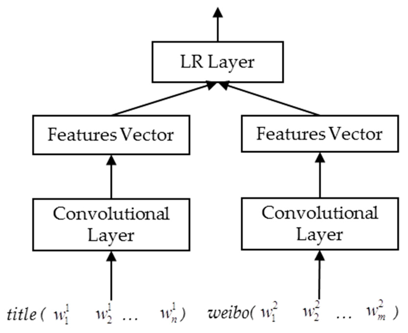
4.2.3. Convolutional Neural Networks (CNN)

CNNs have been validated as being effective in many natural language processing tasks, such as sentiment classification [42], question-answer matching [7] and text entailment [5]. It has the ability to capture local representative structures through convolution and max-pooling. The CNN architecture we adopt in this paper is a modification of ARC-I in a previous study [5], shown in Figure 1. We assumed that a sentence had been expanded with k-dimensional character embeddings and is represented as
w 1 : n = w 1 w 2 , , w n ,
where is the concatenation operator, w a : b stands for { w a , w a + 1 , , w b } and n is the maximum length for sentences in the corpus. CNN operations for sentence modeling include convolution and max-pooling. The convolution operation involves a filter W m h × k , which is a fixed length sliding window, to capture the features in a local view.
c i m = σ ( W m x i : i + h + b m ) , i = 0 , 1 , , n h + 1 ,
where c i m is the convolution result for the ith position in the mth layer, σ is the activation function and bm is the bias factor for layer m. Max-pooling is the operation that selects the unit with the maximum weighted value for a local region. It is appropriate to learn discrete representations for language signals.
c ^ i m = max ( c i m , c i + 1 m , , c i + d 1 m ) , i = 0 , d , 2 d , ,
where d is the region size and a d-max-pooling is used to select the maximum unit in every adjacent d convolutional unit. Usually, a CNN architecture can have multiple convolution and max-pooling layers, with the representations for deeper layers produced in a similar way. The output of CNN is a fixed length vector, standing for the features of a sentence. For identifying document–summary pairs, each document and its summary were considered as two sentences and were converted into two fixed length vectors by CNN separately, then two vectors were concatenated as the features for the document–summary pair and was used for classification (i.e., LR Layer in Figure 1).

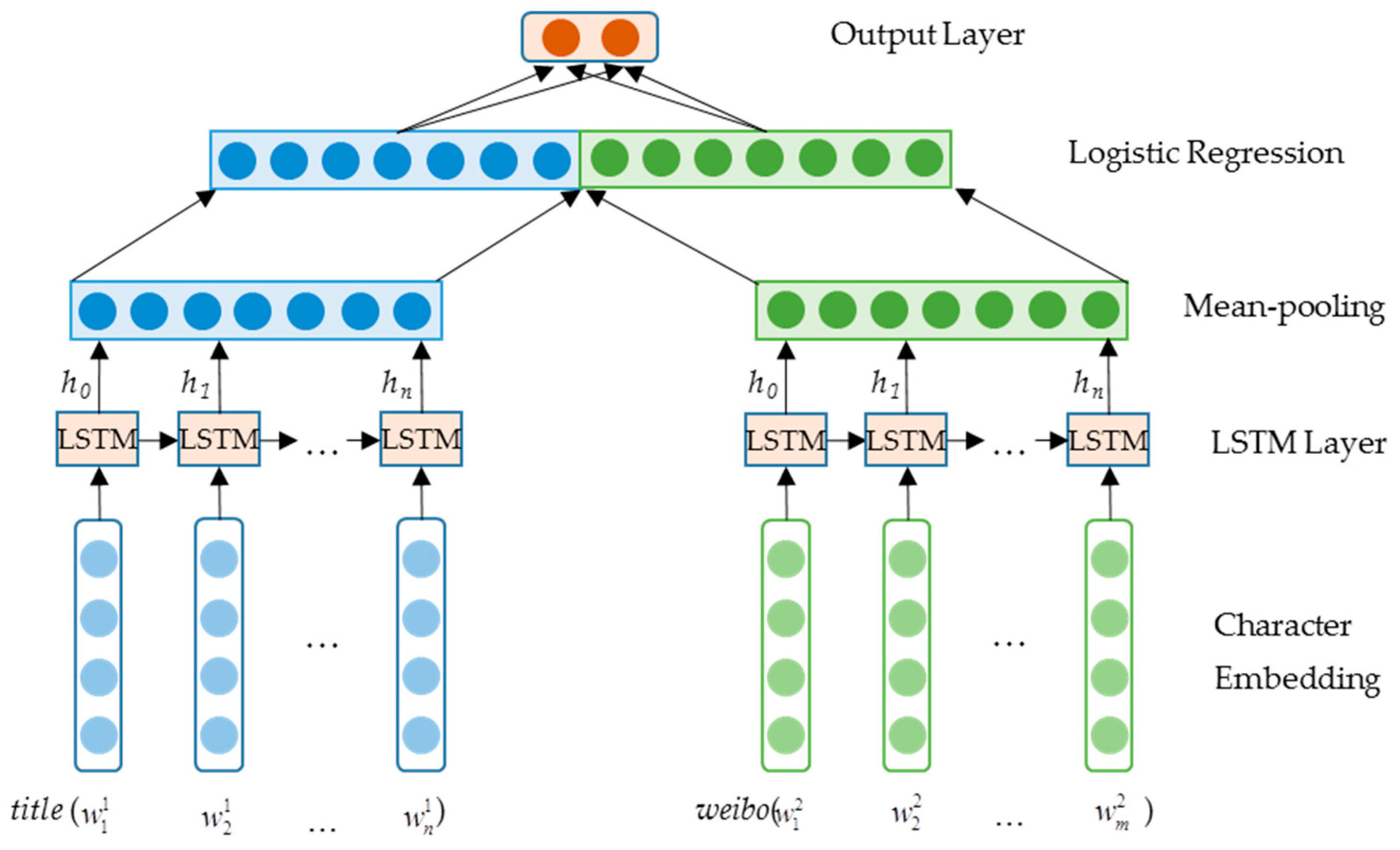
4.3. Long Short-Term Memory (LSTM)
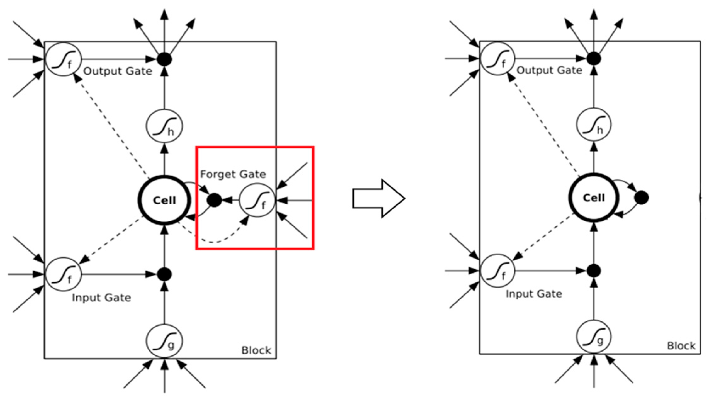
The LSTM-based architecture is analogous to the RNN-based one. The main difference is that LSTM is used to encode the input sentences into feature vectors. We denote this architecture as LSTM-I with its overview shown in Figure 2. In the input phase, each character is expanded into a vector with character embeddings. As a sequential input, each character in the sentence is taken as the input signal for each time step. LSTM, the recurrent neural network, receives signals in each step and accumulates the representations with the propagation of information. A mean-pooling layer is appended so that the information along the whole sequence can be retained. Finally, a logistical layer is used for prediction.
Concretely, a LSTM unit is constituted by an input gate (it), an output gate (ot), a forget gate (ft) and a memory cell (ct), with mathematical equations as follows.
i t = σ ( W i x t + U i h t 1 + b i ) ,
c ˜ t = t a n h ( W c x t + U c h t 1 + b c ) ,
f t = σ ( W f x t + U f h t 1 + b f ) ,
o t = σ ( W o x t + U o h t 1 + b o ) ,
c t = i t c ˜ t + f t c t 1 ,
h t = o t t a n h ( c t ) ,
where W, U, and b are weight matrices and biases for each gate and the memory cell, while σ and t a n h are activation functions, and σ is usually set as rectified linear unit [53] or Sigmoid. The memory cell stores the useful information for each step. The input gate determines what would input to the memory cell. The forget gate determines what information should be forgotten, while the output gate determines what information should be passed on to the memory cell. ht is the actual output of the neural unit which is further processed by the following layers.
A mean-pooling layer follows the LSTM layer (Figure 2). In each time step, the information from the start until the current step is accumulated and further added up to the pooling layer. Thus, the pooling layer stores the sequential information. With a mean operation, the sequential information is averaged. When comparing the two types of pooling, mean-pooling has a better ability in preserving information across the whole document, while max-pooling is good at identifying the most representative words or segments in the document. In our task, mean-pooling seemed to be more reasonable because we needed to keep the meanings of all text segments in the memory so that a more complete summary can be generated.

4.4. Improved LSTM

Text summarization is distinct from classification tasks in that it should make use of almost all the information along the input sequence rather than only capturing the most representative part. Although LSTM has a better memory ability compared to the basic RNN architecture, it still forgets some information due to the existence of the multiple gates and the variable length of the sequence. With regards to this issue, we improved the LSTM unit so that more information could be preserved along the timeline.
The forget gate in LSTM plays an important role since it automatically removes the useless parts when information is propagated. It is helpful in tasks where there are multiple noisy features for decisions, such as sentiment analysis. However, in text summarization, LSTM should have the ability to memorize the topics from the first sentence of the document to the end without any omission. Removing the forget gate seems to be a reasonable way to address the issue. Therefore, we just simply removed the forget gate from the LSTM unit (Figure 3) and expected less information loss. The equations for LSTM then become
i t = σ ( W i x t + U i h t 1 + b i ) ,
c ˜ t = t a n h ( W c x t + U c h t 1 + b c ) ,
o t = σ ( W o x t + U o h t 1 + b o ) ,
c t = i t c ˜ t + c t 1 ,
h t = o t t a n h ( c t ) ,

5. Experiments

5.1. Experimental Settings

The statistics for the dataset used was shown in Table 6, with positive samples titled 4′ + 5′ and negative samples titled 1′ + 2′ + 3′. We trained our models using the training set, fine-tuned the parameters using the development set, and validated the performance using the test set.
We used AUC as the evaluation metric. Before introducing AUC, we needed to know about the receiver operating characteristics (ROC) curve, which is produced based on the definition of TP (True Positive), FN (False Negative), FP (False Positive), and TN (True Negative) samples. The two dimensions for the ROC curve are denoted as TPR (True Positive Rate) and FPR (False Positive Rate), which are defined by Equations (19) and (20). Furthermore, AUC is the area surrounded by ROC, ranges from 0 to 1. The ideal case for classification is assigned a value of 1. The advantage of the AUC values lie in that they avoid the setting of thresholds for classification, and thus, reduce the subjective factors.
T P R = T P T P + F N ,
F P R = F P F P + T N ,
We compared performances of ROUGE-based method, LSI, SVM, CNN, GRU, LSTM, bi-LSTM, and improved LSTM method on document–summary pairs identification. The deep neural network-based methods we chose comparison achieved excellent results in previous studies on text pair classification tasks and sentence classification tasks: CNN on sentences matching [5] and question classification [29], GRU on sentiment classification [12]; LSTM on answer selection [8] and textual entailment recognition [10], bi-LSTM on question tile and body relation identifying [46].
Recall-oriented understudy of gisting evaluation (ROUGE) is an evaluation measure for text summarization. It is surface lexical similarity between summary generated automatic and summary human written [54]. The ROUGE-based method for identifying document–summary pairs here used ROUGE score between each document and its summary as quality score for the pair.
To extract features for SVM and LSI, sentences in the datasets were segmented into Chinese words using jieba (https://pypi.python.org/pypi/jieba/). The SVM model was implemented using the library Scikit-learn [51]. Each weibo and its title were converted to a TF–IDF vector separately, and the two vectors were concatenated as one sample vector. The length of the vector was 67,183. The SVM model was trained with the settings: c = 1.0, using radial basis function kernel and enabling probability estimate.
The LSI was implemented using the library Gensim [55], with the topic number set to 400 for the LSI model training. In the training step, the weibo and title were used as independent texts to train the LSI model. In the testing step, similarity between each weibo and its title was computed based on the trained LSI model, and each weibo–title pair was identified based on the similarity.
Deep neural network-based models were implemented with the help of Theano [56]. The character embeddings were pre-trained on the raw data in the LSTSC corpus with the word2vec toolkit [41]. In our study, the dimensions of character embeddings was set to 50, the sentence length was set to 50. For the deep CNN method, one layer of convolution and one layer of max-pooling were used, number of hidden layers was set to 50. For GRU, LSTM-I, bi-LSTM, and LSTM-II methods, Adadelta [57] was used as the method for parameter updating with the constant 1e-5 and the decay rate of 0.95; the batch size for the input samples was set to 16; the epoch was set at 5.
The experiments were arranged as follows: (1) We compared the AUC values to the baselines and the proposed methods to examine the learning ability of LSTM-based models on the training set and the test set; (2) As size of the labeled training set were limited, we considered how the training size would affect the AUC values so that we could further annotate more samples to enhance the current results; (3) For the document–summary pairs identification problem being considered as binary classification problem in our study, we compared the models trained with two-classes dataset and five-classes dataset; (4) As the LSTM units have the ability to retain information as state in Section 4.3, we expected how the results would change with the addition of the dimension of character embeddings. In the experimental section, we denoted the basic LSTM as LSTM-I and the improved LSTM as LSTM-II. (5) We checked whether the high quality document–summary pairs identified by the proposed method were effective in improving the deep neural network based text summarization model.

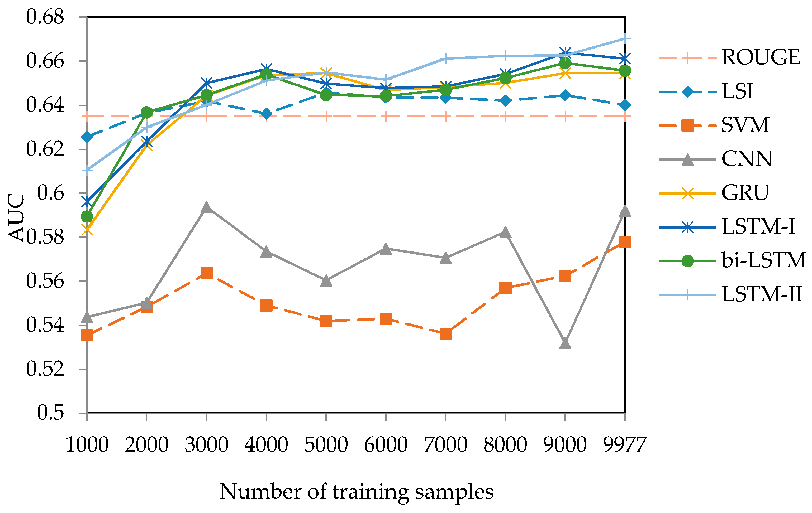
5.2. Experiment Results
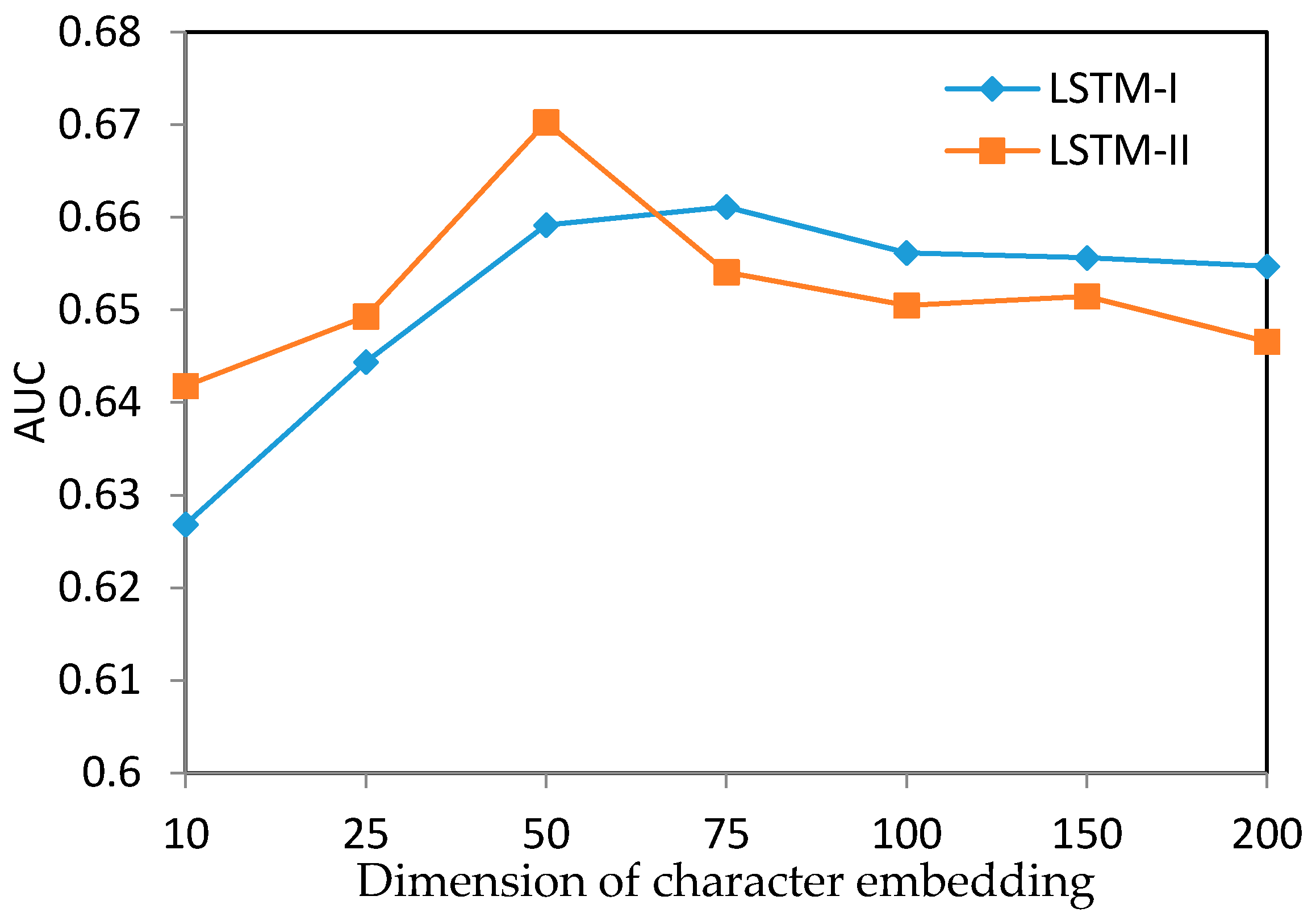
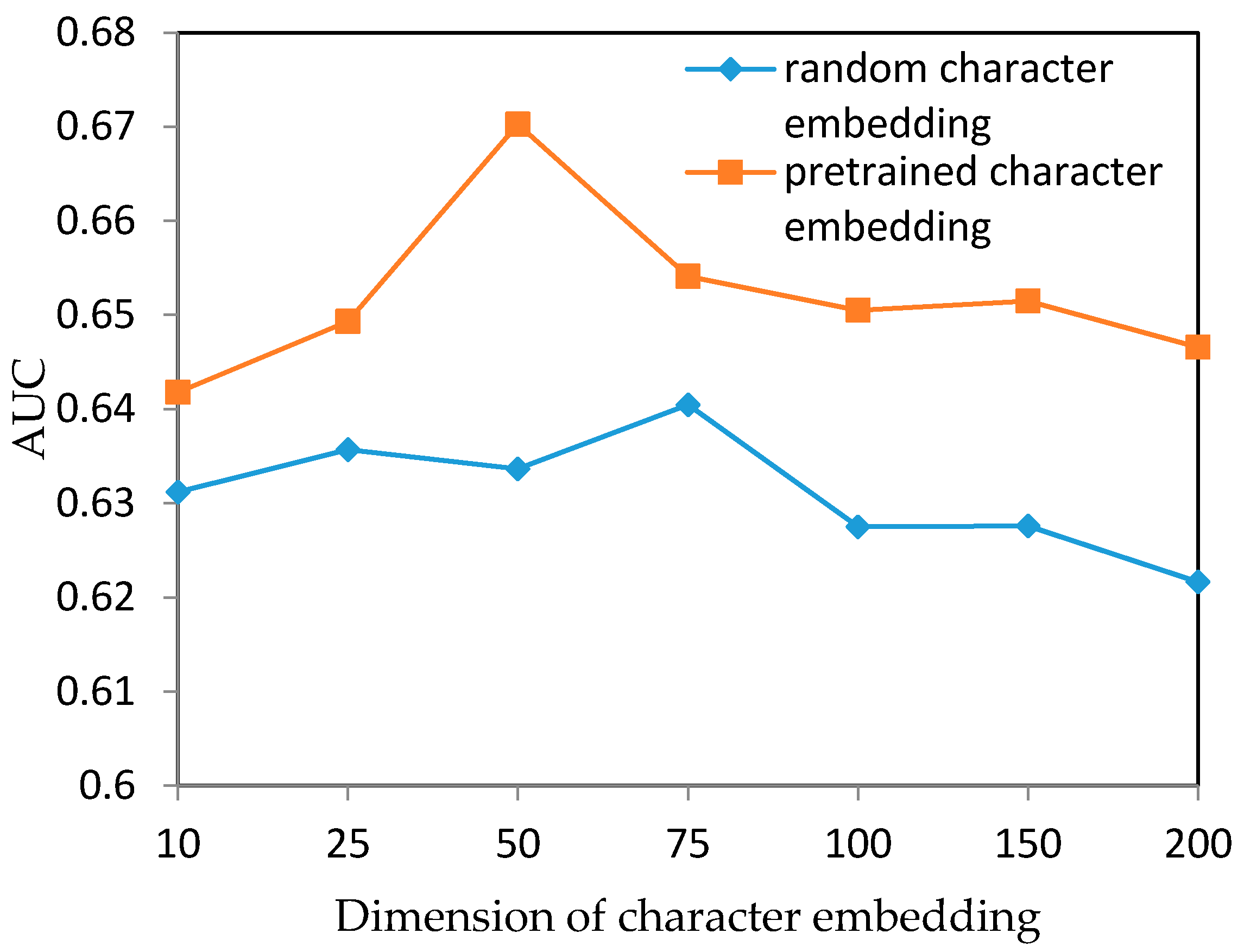
We first ran each method on the training set using 10-fold cross validation and got an average result; and then trained models of each method using the training set and tested each method on the test set. The AUC values of each method were shown in Table 8.
From Table 8 we noticed the performances of each method were consistent on the training set and the test set. The LSTM-based methods outperformed over other baseline methods on the both data sets. The two statistical learning methods, the LSI had an improvement over the SVM 6.36%, indicating the importance of the topic concept and the semantic differences of words. The performance of the method ROUGE was also better than SVM of 5.74% and CNN of 2.97% on the testing set, and even better than LSTM-I of 0.19% on the training set, which showed that the number of common words between document and its summary was an effective feature for identifying document–summary pairs. The results of CNN was not satisfactory mainly due to CNN lacking the capacity of keeping long term memories despite it being able to reserve representative features in a sentence. Hence, CNN only produced a result slightly better than SVM but worse than ROUGE-based method, LSI, GRU, and LSTM-based methods. Performance of the GRU method was better than ROUGE-based method, LSI, SVM, and CNN methods, but worse than the LSTM-based methods on the test set. Performance of Bi-LSTM was worse compared with LSTM-I and LSTM-II with respect to the test set. LSTM-II enhanced LSTM-I by 0.92% on the test set and 1.16% on the training set, and enhanced bi-LSTM by 1.46% on the test set and 0.95% on the training set. We believe LSTM-II was a good demonstration of its superior memory ability.
From Table 8 we found that the performance on the test set was higher than the performance on the training set for all methods that were run. This was caused by the different data annotation strategies on the training set and the test set. For the training set, the annotation aim was to build a large dataset with less annotation work; for the test set, the annotation aim was to ensure the correctness of the dataset. Thus, each pair in the training set was annotated by only one annotator, but each pair in the test set was annotated by three annotators. The correctness of the annotation for the test set was higher than that of the training set.
To check whether the performance of LSTM-II was better than LSTM-I in statistics on the test set, we did significant test between the results of LSTM-I and LSTM-II on the test set, and got value p-value < 0.05, which showed significant difference between the two results. So the performance of LSTM-II was better than LSTM-I on the test set in statistics based on significant test.
We further generated more AUC values and drew curves through an incremental experiment. Random subsets were selected as training data with number of pairs from 1000 to 10000 with an increase of 1000. The curves were shown in Figure 4.
From Figure 4 we could find that GRU and LSTM-based methods were generally better than others with the change of the training set size, indicating the stability of the models. When the sample size was low (< 4000), we found that the curve of ROUGE, LSI, GRU, LSTM-I, and bi-LSTM could sometimes be higher than that of LSTM-II. However, with an increase in samples, LSTM-II performed beyond other methods. Furthermore, we also noticed that when the size of training samples was small (i.e., 1000 and 2000), LSI achieved the best result, which could be explained by the insufficient training of the deep neural networks. The deep models needed a large scale of training data so that the parameters could be fully learned. Therefore, a clear trend for GRU and LSTM-based methods was that the curves were increasing in a linear manner when adding more samples. Comparatively, SVM and LSI had worse results on the AUC curves and there seemed to be less regularities to them. This was particularly the case for LSI as, although it performed well with an increase in training set size, the curve started to decline when training used over 5000 samples. This indicated that LSI possibly might not be able to mine more valuable information through expanding the training scale. The trend of bi-LSTM was similar, and slightly worse, compared to LSTM-I, which meant that the bi-LSTM method could not improve the performance compared to LSTM-I on different sizes of training data. We thought that the possible reason might be a lack of the training data for bi-LSTM, as the number of parameters for bi-LSTM was double that of LSTM-I, or difficulty in optimization for bi-LSTM based on the same sized training data for the document–summary pair identifying tasks.

5.3. Discussion

We further discussed the effects of character embeddings by using different dimensions as well as the performance of random embeddings (Figure 5). We only tested LSTM-I and LSTM-II with the dimension of character embedding ranging from 10 to 200 (small intervals at the beginning and large intervals later because we obtained the best result at dimension 50). It was noticed that the optimal AUC value was achieved when the dimension of the character embedding was 50, with the value decreasing drastically later. The curve of LSTM-I was similar to that of LSTM-II with an increase in embedding dimensions. However, when the information capacity of the character embedding as well as the dimension of LSTM units (we set the dimension of the LSTM units the same as the input character dimension in our models) was low (a low dimension, i.e., <50), we found that LSTM-II got better AUC values. To some extent, it validated the ability of LSTM-II in keeping long-term sequential information.
In the experiments, we used a pre-trained character embedding matrix which was trained on the raw data crawled from Sina Weibo. Since some studies found that using random embeddings as input could also generate good results [29], we tested the contribution of the pre-trained embeddings by comparing with LSTM-II with random input embeddings. We also tried different dimensions analogous to the above experiment, with the curves shown in Figure 6. It was clear to see that the model with pre-trained embeddings was better than that with random embeddings. Pre-training the embeddings was an operation to discover the data distributions on the corpus which was helpful for the model in searching optimal points. We believed that our model also benefits from the pre-trained character embeddings.
The document–summary pairs were annotated with five-score levels in the dataset we used. For the high quality document–summary pairs identification task, we converted these five-score levels data to two-class labels in our experiments. To check the impact of the data classes number converting, we ran an experiment using the five-score levels data directly to training five-class classifier, and compared the performance of the model trained with five-class data with the model trained with two-class data. The results were shown in Table 9. To compute the AUC values for the results of the five-class model, the predicted results with five-class labels were converted to two classes. From the Table 9, it could find that the performance of two-class model was superior to that of five-class model, performance of the LSTM-I model on the two-class data set was improved 0.24% over the five-class data set, and the LSTM-II model was improved 0.62%. The number of samples in each class in two-class data was more than five-class data set as showed in Table 6, which showed that the number of training data in each class had impact on final results, model trained with more number of training samples in each class could obtain better performance under the case of small size training set.

5.4. Case Study

Table 10 showed an example which was identified by LSTM-II method but not by other methods. This weibo contained 76 Chinese characters and it was a typical case with the key words going from the beginning to the end of the document (marked bold in Table 10).
In our experiments, it was proven that the model with 50-dimension input vectors produced the optimal results. Furthermore, it seemed that it was difficult for a model with low input dimensions to retain a larger quantity of information in its memory. From this case, we found the advantage of the LSTM-II in memorizing long term dependences. Through deeper analysis, we discovered that the LSTM-II performed better than the others mainly in the following cases: (1) the length of the document was long (more than 70 characters); (2) Some words were duplicate in semantic meaning for the title and the document but sometimes they were not the same. As an example, this was seen in claimed that the problems were hard and claimed that the examination was hard in Table 10. This case was typical especially when compared with SVM and LSI, indicating the deep models were advantageous in learning semantic distributions for words/characters. (3) The intervals between keywords in the document were relatively large, which was more appropriate for long-term information learning.

5.5. Text Summarization

We further tested the effectiveness of the high quality document–summary pairs for the deep neural network based text summarization model training. Firstly, 1,920,472 high quality document–summary pairs were identified from 2,400,591 raw pairs by the trained LSTM-II model. Secondly, a deep neural network based text summarization model was trained using the identified pairs. Finally, summaries for documents in the test set were generated using the trained text summarization model. We used the same RNN text summarization model and the same parameters setting as those used in Hu et al.’s work [4], which used GRU as the encoder to encode the aim document, and used another GRU as a decoder to generate the summary, and the local context information of the aim document was acquired from the encoding step and was used during decoding. The summaries generated were evaluated with the ROUGE metrics [54], including ROUGE-1, ROUGE-2, and ROUGE-L. The evaluation results of the generated summaries were shown in Table 11.
We compared our text summarization results with the results generated by Hu et al.’s model which trained with all the 2,400,591 raw document–summary pairs in the LCSTS corpus. RNN-context-A was the results from Hu et al.’s work, and RNN-context-B was the results of our trained model. From Table 11, we found that performance of RNN-context-B model was better than RNN-context-A model; the RNN-context-B improved 2.2% on R-L score over RNN-context-A with the number of training pairs less 480,119 than RNN-context-A. The results showed that using high quality document–summary pairs to train the deep neural network based text summarization model could improve the performance, and the high quality document–summary pairs identified by our proposed method was effective for improving the deep text summarization model training.

6. Conclusions

Automatic text summarization based on deep learning generally requires a large scale of effective training data. In this paper, we proposed a novel LSTM-based method to identify the high-quality document–summary pairs from the crawled raw data. We further removed the forget gate in the LSTM unit so as to retain more information from the beginning of the sequence. Experiments showed that the LSTM-based methods outperformed the baseline methods. Removing the forget gate was appropriate for identifying document–summary pairs as the model without the gate also enhanced the basic LSTM model. Experiments on text summarization showed that building high quality pair datasets with the proposed LSTM-II model was effective to improve performance of the deep neural network based text summarization model. In the future, more data will be added for training as well as testing. Furthermore, novel neural network layers will be considered to address the issue of information loss.

Acknowledgments

The work is supported in part by National 863 Program of China (2015AA015405), NSFCs (National Natural Science Foundation of China) (61402128, 61473101, and 61272383), and Strategic Emerging Industry Development Special Funds of Shenzhen (JCYJ20140417172417105 and JCYJ20140508161040764), Program from the Key Laboratory of Symbolic Computation and Knowledge Engineering of Ministry of Education (93K172016K12), and CCF-Tencent Open Research Fund (RAGR20160102). We thank the reviewers for their insightful comments on this paper.

Author Contributions

Yongshuai Hou, Yang Xiang, and Qingcai Chen conceived and designed the experiments; Yongshuai Hou and Fangze Zhu performed the experiments; Yongshuai Hou and Yang Xiang analyzed the data; Yongshuai Hou wrote the paper, Buzhou Tang and Xiaolong Wang checked and modified the paper. All authors have read and approved the final manuscript.

Conflicts of Interest

The authors declare no conflict of interest. The founding sponsors had no role in the design of the study; in the collection, analyses, or interpretation of data; in the writing of the manuscript, or in the decision to publish the results.

References

  1. Hovy, E.; Lin, C.Y. Automated Text Summarization and the SUMMARIST System. In Proceedings of the Workshop on TIPSTER’98, Baltimore, MD, USA, 13–15 October 1998; pp. 197–214. [Google Scholar]
  2. Gambhir, M.; Gupta, V. Recent automatic text summarization techniques: A survey. Artif. Intell. Rev. 2017, 47, 1–66. [Google Scholar] [CrossRef]
  3. Bhatia, N.; Jaiswal, A. Trends in extractive and abstractive techniques in text summarization. Int. J. Comput. Appl. 2015, 117, 21–24. [Google Scholar] [CrossRef]
  4. Hu, B.; Chen, Q.; Zhu, F. LCSTS: A Large Scale Chinese Short Text Summarization Dataset. In Proceedings of the 2015 Conference on Empirical Methods in Natural Language Processing, Lisbon, Portugal, 17–21 September 2015; pp. 1967–1972. [Google Scholar]
  5. Hu, B.; Lu, Z.; Li, H.; Chen, Q. Convolutional Neural Network Architectures for Matching Natural Language Sentences. arXiv, 2015; arXiv:1503.03244. [Google Scholar]
  6. Bahdanau, D.; Cho, K.; Bengio, Y. Neural Machine Translation by Jointly Learning to Align and Translate. arXiv, 2014; arXiv:1409.0473. [Google Scholar]
  7. Yu, L.; Hermann, K.M.; Blunsom, P.; Pulman, S. Deep Learning for Answer Sentence Selection. arXiv, 2014; arXiv:1412.1632. [Google Scholar]
  8. Zhou, X.; Hu, B.; Chen, Q.; Tang, B.; Wang, X. Answer Sequence Learning with Neural Networks for Answer Selection in Community Question Answering. arXiv, 2015; arXiv:1506.06490. [Google Scholar]
  9. Zhou, X.; Hu, B.; Chen, Q.; Wang, X. An Auto-Encoder for Learning Conversation Representation Using LSTM. In Proceedings of the International Conference on Neural Information Processing, Istanbul, Turkey, 9–12 November 2015; pp. 310–317. [Google Scholar]
  10. Liu, P.; Qiu, X.; Chen, J.; Huang, X. Deep Fusion LSTMs for Text Semantic Matching. In Proceedings of the 54th Annual Meeting of the Association for Computational Linguistics, Berlin, Germany, 7–12 August 2016; pp. 1034–1043. [Google Scholar]
  11. Chung, J.; Gulcehre, C.; Cho, K.; Bengio, Y. Empirical Evaluation of Gated Recurrent Neural Networks on Sequence Modeling. arXiv, 2014; arXiv:1412.3555. [Google Scholar]
  12. Tang, D.; Qin, B.; Liu, T. Document Modeling with Gated Recurrent Neural Network for Sentiment Classification. In Proceedings of the 2015 Conference on Empirical Methods in Natural Language Processing, Lisbon, Portugal, 17–21 September 2015; pp. 1422–1432. [Google Scholar]
  13. Hochreiter, S.; Schmidhuber, J. Long short-term memory. Neural Comput. 1997, 9, 1735–1780. [Google Scholar] [CrossRef] [PubMed]
  14. Das, D.; Martins, A.F. A survey on automatic text summarization. Lit. Surv. Lang. Stat. II Course CMU 2007, 4, 192–195. [Google Scholar]
  15. Saranyamol, C.; Sindhu, L. A survey on automatic text summarization. Int. J. Comput. Sci. Inf. Technol. 2014, 5, 7889–7893. [Google Scholar]
  16. Schluter, N.; Søgaard, A. Unsupervised extractive summarization via coverage maximization with syntactic and semantic concepts. In Proceedings of the 53rd Annual Meeting of the Association for Computational Linguistics and the 7th International Joint Conference on Natural Language Processing, Beijing, China, 26–31 July 2015; pp. 840–844. [Google Scholar]
  17. Cao, Z.; Wei, F.; Li, S.; Li, W.; Zhou, M.; Wang, H. Learning Summary Prior Representation for Extractive Summarization. In Proceedings of the 53rd Annual Meeting of the Association for Computational Linguistics and the 7th International Joint Conference on Natural Language, Beijing, China, 26–31 July 2015; pp. 829–833. [Google Scholar]
  18. Yogatama, D.; Liu, F.; Smith, N.A. Extractive Summarization by Maximizing Semantic Volume. In Proceedings of the 2015 Conference on Empirical Methods in Natural Language Processing, Lisbon, Portugal, 17–21 September 2015; pp. 1961–1966. [Google Scholar]
  19. Ganesan, K.; Zhai, C.; Han, J. Opinosis: A Graph-based Approach to Abstractive Summarization of Highly Redundant Opinions. In Proceedings of the 23rd International Conference on Computational Linguistics, Beijing, China, 23–27 August 2010; pp. 340–348. [Google Scholar]
  20. Li, W. Abstractive Multi-document Summarization with Semantic Information Extraction. In Proceedings of the 2015 Conference on Empirical Methods in Natural Language Processing, Lisbon, Portugal, 17–21 September 2015; pp. 1908–1913. [Google Scholar]
  21. Nallapati, R.; Zhou, B.; Gulcehre, C.; Xiang, B. Abstractive Text Summarization Using Sequence-to-Sequence RNNs and Beyond. arXiv, 2016; arXiv:1602.06023. [Google Scholar]
  22. Fuentes, M.; Alfonseca, E.; Rodríguez, H. Support vector machines for query-focused summarization trained and evaluated on pyramid data. In Proceedings of the 45th Annual Meeting of the ACL on Interactive Poster and Demonstration Sessions; Association for Computational Linguistics, Prague, Czech Republic, 25–27 June 2007; pp. 57–60. [Google Scholar]
  23. Wong, K.F.; Wu, M.; Li, W. Extractive summarization using supervised and semi-supervised learning. In Proceedings of the 22nd International Conference on Computational Linguistics-Volume 1; Association for Computational Linguistics, Manchester, UK, 18–22 August 2008; pp. 985–992. [Google Scholar]
  24. Erkan, G.; Radev, D.R. Lexrank: Graph-based lexical centrality as salience in text summarization. J. Artif. Intell. Res. 2004, 22, 457–479. [Google Scholar]
  25. Mihalcea, R. Graph-based Ranking Algorithms for Sentence Extraction, Applied to Text Summarization. In Proceedings of the ACL 2004 on Interactive Poster and Demonstration Sessions, ACLdemo’04, Barcelona, Spain, 21–26 July 2004. [Google Scholar]
  26. Hatzivassiloglou, V.; Klavans, J.L.; Holcombe, M.L.; Barzilay, R.; Kan, M.Y.; McKeown, K.R. Simfinder: A flexible clustering tool for summarization. In Proceedings of the NAACL Workshop on Automatic Summarization, Pittsburgh, PA, USA, 2–7 June 2001. [Google Scholar]
  27. Llewellyn, C.; Grover, C.; Oberlander, J. Improving Topic Model Clustering of Newspaper Comments for Summarisation. In Proceedings of the ACL 2016 Student Research Workshop, Berlin, Germany, 7–12 August 2016; pp. 43–50. [Google Scholar]
  28. Hochreiter, S.; Bengio, Y.; Frasconi, P.; Schmidhuber, J. Gradient Flow in Recurrent Nets: The Difficulty of Learning Long-Term Dependencies; IEEE Press: Hoboken, NJ, USA, 2001. [Google Scholar]
  29. Kim, Y. Convolutional neural networks for sentence classification. arXiv, 2014; arXiv:1408.5882. [Google Scholar]
  30. Rush, A.M.; Chopra, S.; Weston, J. A Neural Attention Model for Abstractive Sentence Summarization. In Proceedings of the 2015 Conference on Empirical Methods in Natural Language Processing, Lisbon, Portugal, 17–21 September 2015; pp. 379–389. [Google Scholar]
  31. Cheng, J.; Lapata, M. Neural Summarization by Extracting Sentences and Words. In Proceedings of the 54th Annual Meeting of the Association for Computational Linguistics, Berlin, Germany, 7–12 August 2016; pp. 484–494. [Google Scholar]
  32. Over, P.; Dang, H.; Harman, D. DUC in context. Inf. Process. Manag. 2007, 43, 1506–1520. [Google Scholar] [CrossRef]
  33. Owczarzak, K.; Dang, H.T. Overview of the TAC 2011 summarization track: Guided task and AESOP task. In Proceedings of the Text Analysis Conference (TAC 2011), Gaithersburg, MD, USA, 14–15 November 2011. [Google Scholar]
  34. Napoles, C.; Gormley, M.; Van Durme, B. Annotated Gigaword. In Proceedings of the Joint Workshop on Automatic Knowledge Base Construction and Web-Scale Knowledge Extraction, Montreal, Canada, 7–8 June 2012; pp. 95–100. [Google Scholar]
  35. Nakov, P.; Màrquez, L.; Moschitti, A.; Magdy, W.; Mubarak, H.; Freihat, A.A.; Glass, J.; Randeree, B. SemEval-2016 Task 3: Community Question Answering. In Proceedings of the 10th International Workshop on Semantic Evaluation, San Diego, CA, USA, 16–17 June 2016. [Google Scholar]
  36. Salton, G.; Wong, A.; Yang, C.-S. A vector space model for automatic indexing. Commun. ACM 1975, 18, 613–620. [Google Scholar] [CrossRef]
  37. Deerwester, S.; Dumais, S.T.; Furnas, G.W.; Landauer, T.K.; Harshman, R. Indexing by latent semantic analysis. J. Am. Soc. Inf. Sci. 1990, 41, 391. [Google Scholar] [CrossRef]
  38. Papadimitriou, C.H.; Tamaki, H.; Raghavan, P.; Vempala, S. Latent Semantic Indexing: A Probabilistic Analysis. In Proceedings of the Seventeenth ACM SIGACT-SIGMOD-SIGART Symposium on Principles of Database Systems, New York, NY, USA, 1–4 June 1998; pp. 159–168. [Google Scholar]
  39. Blei, D.M.; Ng, A.Y.; Jordan, M.I. Latent dirichlet allocation. J. Mach. Learn. Res. 2003, 3, 993–1022. [Google Scholar]
  40. Golub, G.H.; Reinsch, C. Singular value decomposition and least squares solutions. Numer. Math. 1970, 14, 403–420. [Google Scholar] [CrossRef]
  41. Mikolov, T.; Chen, K.; Corrado, G.; Dean, J. Efficient Estimation of Word Representations in Vector Space. arXiv, 2013; arXiv:1301.3781. [Google Scholar]
  42. Poria, S.; Cambria, E.; Gelbukh, A. Deep Convolutional Neural Network Textual Features and Multiple Kernel Learning for Utterance-level Multimodal Sentiment Analysis. In Proceedings of the 2015 Conference on Empirical Methods in Natural Language Processing, Lisbon, Portugal, 17–21 September 2015; pp. 2539–2544. [Google Scholar]
  43. Poria, S.; Cambria, E.; Gelbukh, A. Aspect extraction for opinion mining with a deep convolutional neural network. Knowl. Based Syst. 2016, 108, 42–49. [Google Scholar] [CrossRef]
  44. Wang, B.; Liu, K.; Zhao, J. Inner Attention based Recurrent Neural Networks for Answer Selection. In Proceedings of the 54th Annual Meeting of the Association for Computational Linguistics, Berlin, Germany, 7–12 August 2016; pp. 1288–1297. [Google Scholar]
  45. Tan, M.; dos Santos, C.; Xiang, B.; Zhou, B. Improved Representation Learning for Question Answer Matching. In Proceedings of the 54th Annual Meeting of the Association for Computational Linguistics, Berlin, Germany, 7–12 August 2016; pp. 464–473. [Google Scholar]
  46. Nie, Y.; An, C.; Huang, J.; Yan, Z.; Han, Y. A Bidirectional LSTM Model for Question Title and Body Analysis in Question Answering. In Proceedings of the 2016 IEEE First International Conference on Data Science in Cyberspace, Changsha, China, 13–16 June 2016; pp. 307–311. [Google Scholar]
  47. Zhang, Z.; Yao, D.; Pang, Y.; Lu, X. Chinese Textual Entailment Recognition Enhanced with Word Embedding; Springer International Publishing: Cham, Switzerland, 2015; pp. 89–100. [Google Scholar]
  48. Lyu, C.; Lu, Y.; Ji, D.; Chen, B. Deep Learning for Textual Entailment Recognition. In Proceedings of the 2015 IEEE 27th International Conference on Tools with Artificial Intelligence, Salerno, Italia, 9–11 November 2015; pp. 154–161. [Google Scholar]
  49. Rocktäschel, T.; Grefenstette, E.; Hermann, K.M.; Kočiský, T.; Blunsom, P. Reasoning about Entailment with Neural Attention. arXiv, 2015; arXiv:1509.06664. [Google Scholar]
  50. Vapnik, V.; Guyon, I.; Hastie, T. Support vector machines. Mach. Learn. 1995, 20, 273–297. [Google Scholar]
  51. Pedregosa, F.; Varoquaux, G.; Gramfort, A.; Michel, V.; Thirion, B.; Grisel, O.; Blondel, M.; Prettenhofer, P.; Weiss, R.; Dubourg, V.; et al. Scikit-learn: Machine Learning in Python. J. Mach. Learn. Res. 2011, 12, 2825–2830. [Google Scholar]
  52. Landauer, T.K.; Foltz, P.W.; Laham, D. An introduction to latent semantic analysis. Discourse Process. 1998, 25, 259–284. [Google Scholar] [CrossRef]
  53. Dahl, G.E.; Sainath, T.N.; Hinton, G.E. Improving deep neural networks for LVCSR using rectified linear units and dropout. In Proceedings of the 2013 IEEE International Conference on Acoustics, Speech and Signal Processing, Vancouver, Canada, 26–31 May 2013; pp. 8609–8613. [Google Scholar]
  54. Lin, C.Y. Rouge: A package for automatic evaluation of summaries. In Proceedings of the Workshop on Text Summarization Branches Out, Barcelona, Spain, 25–26 July 2004. [Google Scholar]
  55. Řehůřek, R.; Sojka, P. Software Framework for Topic Modelling with Large Corpora. In Proceedings of the LREC 2010 Workshop on New Challenges for NLP Frameworks, ELRA, Valletta, Malta, 22 May 2010; pp. 45–50. [Google Scholar]
  56. Theano Development Team. Theano: A Python framework for fast computation of mathematical expressions. arXiv, 2016; arXiv:160502688T.
  57. Zeiler, M.D. ADADELTA: An Adaptive Learning Rate Method. arXiv, 2012; arXiv:1212.5701. [Google Scholar]
Figure 1. The convolutional neural networks (CNN) architecture implemented for document–summary pairs identification.
Information 08 00064 g001
Figure 2. The architecture of the long short-term memory (LSTM)-based model for document–summary pairs identification.
Information 08 00064 g002
Figure 3. The architecture of the source LSTM unit (left) and the improved LSTM unit (right).
Information 08 00064 g003
Figure 4. AUC Curves with an increase in the number of training samples for different methods on the test set.
Information 08 00064 g004
Figure 5. AUC curves with an increase in character embedding dimensions for the LSTM-I and LSTM-II methods.
Information 08 00064 g005
Figure 6. AUC curves of LSTM-II using random character embeddings and pre-trained embeddings.
Information 08 00064 g006
Table 1. An example document and its summary from Sina Weibo.
SummaryDocument
The CVs from postgraduate students were rejected. The company said: undergraduate students were enough.On the 6th, the job fair for graduate students majoring in science and technology was held in Jiangsu Province. During the fair, the CV from a postgraduate student named Xie was refused because the employer said an undergraduate student was enough. Many companies also declared that they would only need undergraduates. Some postgraduates exclaimed that they found that it was more difficult to be employed, despite having learned three years more. Do you agree?
Table 2. An example of noisy pair from Sina Weibo, with the summary being a selection clause from its document.
SummaryDocument
The accumulated number of organ donation in our country reached 5384Until 9th November, the accumulated number of organ donation in our country reached 5384 and the total number of donated organs reached 14,721. However, currently there are only 169 hospitals around China that has at least one qualifications for organ transplantation, with only over 20 surgeons having the ability to do heart and lung transplantations. As China has stepped into the international organ transplant family, our top priority is to cultivate transplant medicine talents.
Table 3. An example of noisy pair from Sina Weibo, with the summary being a comment of its document.
SummaryDocument
Are you a middle-class person?The family finance investigation by Southwestern University of Finance and Economics in 2015 showed: In 2015, the average property for a Chinese family was 919 thousand RMB (China yuan), 69.2% of which were house properties. An adult person from a Chinese middle-class family has an average of 127 thousand dollars (about 810 thousand RMB), which accounts for 21.4% in the adult population.
Table 4. An example of noisy pair from Sina Weibo, with the summary only covering half of the document.
SummaryDocument
The schedule of “Die Hard 5” was determined, being premiered on March 14 nationwide“Die Hard 5” officially announced as screening in the mainland cinema on March 14. This series have gone through 25 glorious years, and won the love of the world fans. The film has taken more than $200 million in overseas box offices in just two weeks. Bruce Willis, aged 58 years old, will powerfully return, will fight terrorists once again and help his son this time.
Table 5. An example of a useful pair from Sina Weibo, with the summary being an abstractive of its document.
TitleDocument
Those superior “foreign hospitals” have difficulty in landing.The policy for hospitals of foreign and individual properties has been attempted for over a year, but there is only one newly established hospital. Constrained by the medical system and market concept, most of them are acclimatized currently. The primary affairs of these hospitals are still international-transfer treatments and medical training cooperation for senior markets, with the landing in most areas still needing time.
Table 6. The quality score of document–summary pair distribution among the datasets.
Dataset1′2′3′1′ + 2′ + 3′4′5′4′ + 5′
Train87797618753728293233176249
Develop6463144271197211408
Test178216227521301197498
Table 7. The document length (in word) distribution among the training set.
Document LengthDocument CountProportion (%)
0~1940.04
20~293843.85
30~39371832.27
40~49519252.04
50~806796.81
total9977100
Table 8. Results of different methods for identifying document–summary pairs on the training set and the test set.
MethodTraining Set (AUC)Test Set (AUC)
ROUGE-based0.62210.6351
LSI0.61600.6413
SVM0.53040.5777
CNN0.52170.6054
GRU0.61860.6545
LSTM-I0.62020.6611
bi-LSTM0.62230.6557
LSTM-II0.63180.6703
Table 9. Results of models trained with two-class data set and five-class data set to identify document–summary pairs.
Data SetLSTM-I (AUC)LSTM-II (AUC)
Five-Class0.65870.6640
Two-Class0.66110.6702
Table 10. An example document–summary pair correctly identified by LSTM-II but failed by other methods.
SummaryDocument
Hundreds of primary school students participated in the “little TOEFL” examination, even top students in English claimed that the problems were hard.At 9 a.m. on the 23th, the ETSTOEFL Junior examination, which is also known as the “little TOEFL” began in Jiangcheng City and it was the first examination. It attracted participants from hundreds of students from primary schools. The “little TOEFL” needs comprehensive abilities of listening, speaking, reading and writing as well as focusing more on practice. Many top students in English claimed that the examination was hard.
Table 11. Evaluation results of summaries generated by models trained with raw pairs and with identified high quality pairs.
ModelTraining Pairs NumberR-1R-2R-L
RNN-context-A [4]2,400,5910.2990.1740.272
RNN-context-B1,920,4720.3120.1950.294

