Reliability Analysis of the High-speed Train Bearing Based on Wiener Process

Abstract

Because of the existence of uncertainty measurement in the process of bearings degradation, it is difficult to carry out the reliability analysis. The random performance degradation model is used to analyze the reliability life of high-speed train bearing with the characteristics of slow degradation process and relatively stable degradation path. The unknown coefficients are viewed as random variables in the model. According to the analysis to a bearing testing data, the reliability analysis of the bearing life is finally completed. The results show that the method can assess reliability of the bearing life with zero failure by taking full advantage of the performance degradation data in the small sample size.

1. Introduction

The requirements for the performance and reliability of key devices are increasing as the complexity of modern industrial equipment increases. The complex equipment is mechanical and has multiple parts. Its working performance changes as the service cycle increases or as environmental stress changes. That is, common degradation, wear, and so on will occur.

With the development of modern information acquisition technology, it is relatively easy for the signal of the system to degrade. However, the degenerate signals generally have random characteristics in practice, such as the fatigue crack growth of metal, the reduction of gyroscope precision, and the reduction of lithium battery capacity. Therefore, it is very difficult and sometimes even impossible to obtain the results of its reliability assessment for a stochastic degradation system.

In fact, uncertainty measurement and individual differences between systems widely vary in the process of system degradation, resulting in uncertainty of system reliability. Integrating the influence of uncertainty measurement and individual differences into reliability analysis to achieve more accurate reliability analysis of stochastic degradation systems is worth studying. In recent years, many scholars have been devoted to this [1,2,3,4,5,6,7,8]. Zhang [4] models the degradation state evolution of a system through a diffusion process with piecewise but time-dependent drift coefficient functions. A numerical study and a case study of Li-ion batteries were carried out to illustrate and demonstrate the proposed prognostic method. Pan et al. [6,7,8] analyzed product reliability using accelerated degradation modeling based on Wiener and gamma processes with fewer pan re-products. Zheng et al. [5] built a nonlinear degradation model based on a nonlinear diffusion degradation process to incorporate the uncertainty measurement and the unit-to-unit variability into the estimated RUL. To analyze the reliability of the light emitting diode, Wang [9] studied the two types of lifetime prediction based on gamma processes. Tsai [10] used the gamma process to provide information about the reliability of highly reliable products that are not likely to fail within a reasonable period of time under traditional life tests, or even accelerated life tests. Although the Wiener process has been widely applied in terms of degradation modeling, in all of the above models, the parameters’ estimation was commonly based on the same distribution and large sample. The individual differences were not considered, and the performance degradation analysis was limited by a small sample.

In this paper, according to the range of performance degradation and engineering experience, a random performance degradation model with a slow degradation process and a relatively stable degradation path, where the unknown coefficients are viewed as random variables, was employed to analyze the reliability of the high-speed train bearing (HSTB). We then made a corrective estimation for the parameters of the model by adopting the maximum likelihood estimation method to solve the problem of a small sample. The reliability function was then determined. By using the living test data of a type of bearing, we verified the feasibility of the above method. The results show that the method can assess reliability of the bearing life with zero failure by taking full advantage of the performance degradation data in the small sample size.

Section 2 first constructs a random performance degradation model with both the random performance degradation and individual differences. An estimation method for the unknown parameters in the model and a solution to the question of a small sample are presented in Section 3. Section 4 provides an example to verify the validity of the reliability model, and Section 5 concludes the paper.

2. Random Degradation Model

2.1. Model Assumption

The degradation model satisfies the following assumptions:

• Product failure is caused by degradation, and degradation failure shows that the change trend of a certain performance parameter is monotonous over time. Let Z(t) denote the performance parameter value at time t. The measured data, written as X(t), corresponding to Z(t), are called “degraded.” The measured error is written as ε(t). Thus, we have Z(t) = X(t) + ε(t). In this paper, we would not consider the measured error, i.e., Z(t) = X(t).
• The tested samples are randomly selected. The test condition and the measurement errors of all products are the same.
• The observed values of the performance parameters obey the independent and identical distribution at all times, whether it is continuous damage or is discrete. The measure is nondestructive.
• The product is identified as a failure when the performance degradation value increases to the failure threshold l.

2.2. Degradation Model

If there are n samples measured in the performance degradation test, the m-fold measures of test data are respectively made at times t₁, t₂, …, t_m. Thus, the performance degradation data are obtained as follows:

X₁(t₁), X₁(t₂), …, X₁(t_m)
   X₂(t₁), X₂(t₂), …, X₂(t_m)
   …  …  …  …
   X_n(t₁), X_n(t₂), …, X_n(t_m)

where X_i(t_j) is the performance degradation value for the ith sample at time t_j, i = 1, 2, …, n, and j = 1, 2, …, m. According to Assumption III, we know that X₁(t_i), X₂(t_i), …, X_n(t_i) obey the independent and identical distribution.

To estimate the sample reliability, we process for the obtained data. The detailed procedure is as follows:

(1)

Collect the degradation data, make the statistical analysis, remove the anomalous data, and judge which distribution is coincident with the performance degradation value at every moment.

(2)

Solve the average and variance of performance degradation value at all times and finally computing the reliability of the tested bearings.

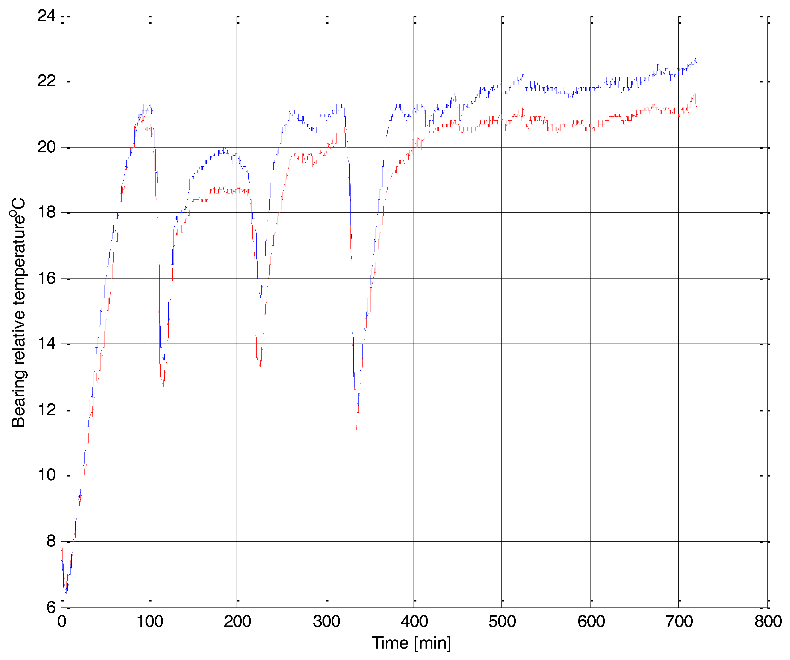
The failure reason is usually too much or too little lubricant, the wear of the cage, or the occurrence of fatigue pitting for the HSTB. However, the external characteristic of failure is the rise of the bearing temperature. Thus, we can forecast the bearing life by viewing the bearing temperature as the parameter of performance degradation. We then randomly select two higher reliability bearings, installed in the same testing machine, to carry out the reliability test, which is conducted in the constant load and speed. The test data are measured nondestructively at the same time and once every 10 s so that Assumptions II and III are confirmed. The tendency chart of the tested bearings about relative temperature, which is relative to the ambient temperature, is shown in Figure 1.

From Figure 1, although we can see three sudden changes in the curve, which are caused by the suspension of the testing machine since the lubrication pressure is under the lower limit of the set value during the test, overall, the bearing’s relative temperature rises slowly with time. This phenomenon reflects the gradual degenerating trend of bearing performance.

We know that, even though the HSTB is a high-reliability and long-life product, the temperature change still shows slow linear rise as time goes on. Relative to an ordinary bearing, the degenerated process is slower, and the degenerated path is more stationary. In addition, as a result of uncertain random factors in the testing environment, there is a rising trend in the curve in Figure 1. In light of the above features of the bearing relative temperature, we used the Wiener process for modeling [6,7,8,9,10,11]. This mathematical model can be expressed as follows:

X(t;v,δ²) = b + vt + δW(t)

(1)

where X(t;v,δ²) is the relative temperature of bearing at time t, b is the initial value of bearing relative temperature, v and δ are unknown parameters, and W(t) is the standard Wiener process, with E[W(t)] = 0, E[W(t₁)W(t₂)] = min(t₁, t₂).

According to Equation (1), we know that the degradation process, i.e., E[X(t)] = b + vt, is linear, so it is often applied to models for products of linear degradation. Nevertheless, it can also be used to describe the nonlinear if we make some transformation for the time variable t.

In Equation (1), if b and v are regarded as constant, the difference cannot be reflected between multiple samples. All samples obey the same distribution. However, they are different in processing technique, manufacturing error, assembling technique, and so on, and the bearing performance is also different in different working environments.

The above problems may cause instability in bearing performance, so the accuracy in the reliability assessment may be reduced if the individual differences are not considered when the sample reliability is evaluated, and it is necessary to describe this uncertain random character. Therefore, we regard b and v as random variables, which obey the normal distribution, i.e., b ~ N(μ_b, ${\sigma }_b^2$), v ~ N(μ_v, ${\sigma }_v^2$).

Most products’ failure in performance will occur as the performance parameter first reaches the failure threshold. The product fails when the performance degradation value X(t) reaches a particular level l. Thus, the failure time T can be defined as [12]

T = inf{X(t) ≥ l, t ≥ 0}.

(2)

For the failure time T, the inverse Gaussian distribution is mainly a description for the time needed to achieve the set distance, so its distribution is defined as the inverse Gaussian distribution in [13]. It is expressed in the following form

$$F\left(t\right)=\Phi \left(\frac{b+vt-l}{\delta \sqrt{t}}\right)+\exp \left(\frac{2\mu l}{{\delta }^2}\right)\Phi (\frac{-b-vt-l}{\delta \sqrt{t}})$$

(3)

where $\Phi \left(t\right)$ is the standard normal distribution function of t. Thus, the probability density function (PDF) of t can be expressed as

$$f\left(t\right)=\sqrt{\frac{l^2}{2\pi {\delta }^2{t}^3}}\exp (-\frac{{(l-b-vt)}^2}{2{\delta }^{2t}})$$

(4)

on the condition of the known failure threshold l, and the parameters b and v are viewed as random variables. We can gain the PDF of bearing life as

$$f\left(t|l\right)={\int }_{-\infty }^{\infty }{\int }_{-\infty }^{\infty }f\left(t\right)\cdot N\left(b|{\mu }_b,{\delta }_b^2\right)\cdot N\left(v|{\mu }_v,{\delta }_v^2\right)dbdv=l/\sqrt{2\pi \left({\delta }^{2}t+{\delta }_b^2+{\delta }_v^2{t}^2\right)}\cdot \exp \left(-\frac{{\left(l-{\mu }_b-{\mu }_{v}t\right)}^2}{2\left({\delta }^{2}t+{\delta }_b^2+{\delta }_b^2{t}^2\right)}\right).$$

(5)

Its distribution function is

$$F\left(t\right)={\int }_{-\infty }^{t}f\left(x|l\right)dx={\int }_{-\infty }^{t}l/\sqrt{2\pi \left({\delta }^{2}x+{\delta }_b^2+{\delta }_v^2{x}^2\right)x^2}\cdot \exp \left(-\frac{{\left(l-{\mu }_b-{\mu }_{v}x\right)}^2}{2\left({\delta }^{2}x+{\delta }_b^2+{\delta }_v^2{x}^2\right)}\right)dx$$

(6)

so the reliability function of bearing can be evaluated by the following integral:

$$R\left(t\right)=1-F\left(t\right)={\int }_t^{\infty }l/\sqrt{2\pi \left({\delta }^{2}x+{\delta }_b^2+{\delta }_v^2{x}^2\right)x^2}\cdot \exp \left(-\frac{{\left(l-{\mu }_b-{\mu }_{v}x\right)}^2}{2\left({\delta }^{2}x+{\delta }_b^2+{\delta }_v^2{x}^2\right)}\right)dx.$$

(7)

3. Parameter Estimation

After arranging for the collected test data, we get the bearing relative temperature X_i(t_j) for the ith test sample at time t_j, so we take points from the above bearing relative temperature data as follows: (t₀, X_i(t₀)), (t₁, X_i(t₁)), …, (t_k, X_i(t_k)), and t₀ ≤ t₁ ≤ … ≤ t_k ≤t_m. It is noted that X_i = [X_i(t₀), X_i(t₁), …, X_i(t_k)] [14,15].

By Equation (1), for the ith test sample, we have

Δx_ij = v_iΔt_j + δ_iΔW(t_j)

(8)

where Δx_ij = X_i(t_j) − X_i(t_j−1), Δt_j=t_j − t_j−1, ΔW(t_j)=W(t_j) − W(t_j−1), i = 1, 2, …, n, and j = 1, 2, …, k.

According to the Wiener process, ΔW(t_j) ~ N(0, Δt_j), so we have

Δx_ij ~ N(v_iΔt_j, δ_i²Δt_j)

(9)

and the Wiener process has the property of stationary independent increments, so we can obtain the joint PDF about Δx_i1, Δx_i2, …, Δx_ik; i.e., the sample likelihood function is

L(v_i, δ_i) = f(Δx_i1, Δx_i2, …, Δx_ik)= f(Δx_i1)f(Δx_i2)…f(Δx_ik).

(20)

Substituting Equation (9) in Equation (10), and taking logarithm on both sides of the equal sign in (10), we get

$$\ln L\left(v_i,{\delta }_i\right)=\ln {\displaystyle \prod _{j=1}^k}f\left(\Delta t_j\right)={\displaystyle \sum _{j=1}^k}(\ln \frac{1}{\sqrt{2\pi {\delta }_i^2\Delta t_j}}-\frac{{\left(\Delta x_{ij}-v_i\Delta t_j\right)}^2}{2{\delta }_i^2\Delta t_j}).$$

(11)

Calculating separately the partial derivative to v_i and δ_i in Equation (11), we get

$$\frac{\partial \ln L}{\partial v_i}={\displaystyle \sum _{j=1}^k}\frac{\Delta x_{ij}-v_i\Delta t_j}{{\delta }_i^2\Delta t_j}=0$$

(12)

$$\frac{\partial \ln L}{\partial {\delta }_i}={\displaystyle \sum _{j=1}^k}(-\frac{1}{{\delta }_i}+\frac{{\left(\Delta x_{ij}-v_i\Delta t_j\right)}^2}{{\delta }_i^3\Delta t_j})=0.$$

(13)

Thus, by solving Equations (12) and (13), we get the maximum likelihood estimate of v_i and δ_i as follows:

$${\widehat{v}}_i=\frac{1}{k}{\displaystyle \sum _{j=1}^k}\frac{\Delta x_{ij}}{\Delta t_j}$$

(14)

$${\widehat{\delta }}_i={\left[\frac{1}{k}{\displaystyle \sum _{j=1}^k}\frac{{\left(\Delta x_{ij}-{\widehat{v}}_i\Delta t_j\right)}^2}{\Delta t_j}\right]}^{\frac{1}{2}}.$$

(15)

Assuming the sample size is n, from Equations (8)–(15), we can get the drifting coefficient $D_v=\{{\widehat{v}}_1,{\widehat{v}}_2,\cdots ,{\widehat{v}}_n\}$ and diffusion coefficient $D_{\delta }=\{{\widehat{\delta }}_1,{\widehat{\delta }}_2,\cdots ,{\widehat{\delta }}_n\}$ of every test sample, and the original value of bearing relative temperature is $D_b=\{b_1,b_2,\cdots ,b_n\}$. ${\widehat{v}}_i$ and ${\widehat{\delta }}_i$ is the estimating value of drifting coefficient and the diffusion coefficient of the ith bearing, respectively, and b_i is the original temperature of the ith bearing, i = 1, 2, …, n.

We can then calculate the estimating values of μ_b, ${\sigma }_b^2$, μ_v, and ${\sigma }_v^2$, which are as follows:

$${\widehat{\mu }}_b=\frac{1}{n}{\displaystyle \sum _{i=1}^n}{b}_i,{\widehat{\sigma }}_b^2=\frac{1}{n}{\displaystyle \sum _{i=1}^n}{\left[b_i-{\widehat{\mu }}_b\right]}^2$$

$${\widehat{\mu }}_v=\frac{1}{n}{\displaystyle \sum _{i=1}^n}{\widehat{v}}_i,{\widehat{\sigma }}_v^2=\frac{1}{n}{\displaystyle \sum _{i=1}^n}{\left[{\widehat{v}}_i-{\widehat{\mu }}_v\right]}^2.$$

At the same time, the estimation of diffusion coefficient $\overline{\delta }$ is defined as the average of the diffusion coefficient $\delta$ of all test samples. That is, $\overline{\delta }=E(\widehat{\delta })=\frac{1}{n}{\displaystyle \sum _{i=1}^n{\delta }_i}$.

Substituting them in Equation (7), we get

$$R\left(t\right)={\int }_t^{\infty }\frac{l}{\sqrt{2\pi ({\overline{\delta }}^{2}x+{\widehat{\delta }}_b^2+{\widehat{\delta }}_v^2{x}^2)x^2}}\cdot \exp \left(-\frac{{(l-{\widehat{\mu }}_b-{\widehat{\mu }}_{v}x)}^2}{2({\overline{\delta }}^{2}x+{\widehat{\delta }}_b^2+{\widehat{\delta }}_v^2{x}^2)}\right)dx$$

(16)

4. Example Analysis

Since the HSTB test is still in the design stage, it is unable to provide the required test data for verifying the validity of the above method. Consequently, we used the test data of two bearings that are similar to the HSTB, shown in Figure 1, as an example to carry out our analysis. The initial values of the bearing relative temperature are b(1) = −0.2 °C and b(2) = −0.9 °C. After the data points from the test data were extracted every minute and the abnormal data were removed, we had 245 degradation data points shown in Figure 2.

For the HSTB, considering that it is hard to obtain good data in a short time since the reliability requirement is higher, the degradation rate is smaller, the degradation process is also slower, and the design index requirement requires a year for the bench test, so we can extend the interval time of data point extraction, such as once every 12 h or every other day, to obtain more effective performance degradation data.

According to Equations (14) and (15), the estimated values of the drift parameters v and the diffusion parameters $\delta$ are obtained.

$$\widehat{v}(1)=0.019,\widehat{\delta }(1)=0.1142$$

$$\widehat{v}(2)=0.025,\widehat{\delta }(2)=0.1141.$$

By calculation, we have

$${\widehat{\mu }}_b=-0.55,{\widehat{\sigma }}_b^2=0.097$$

$${\widehat{\mu }}_v=-0.003,{\widehat{\sigma }}_v^2=2.27\times {10}^{-6}.$$

Then, averaging for the diffusion coefficients of bearings, we get

$$\overline{\delta }=(\hat{\delta }(1)+\hat{\delta }(2)/2=0.11415.$$

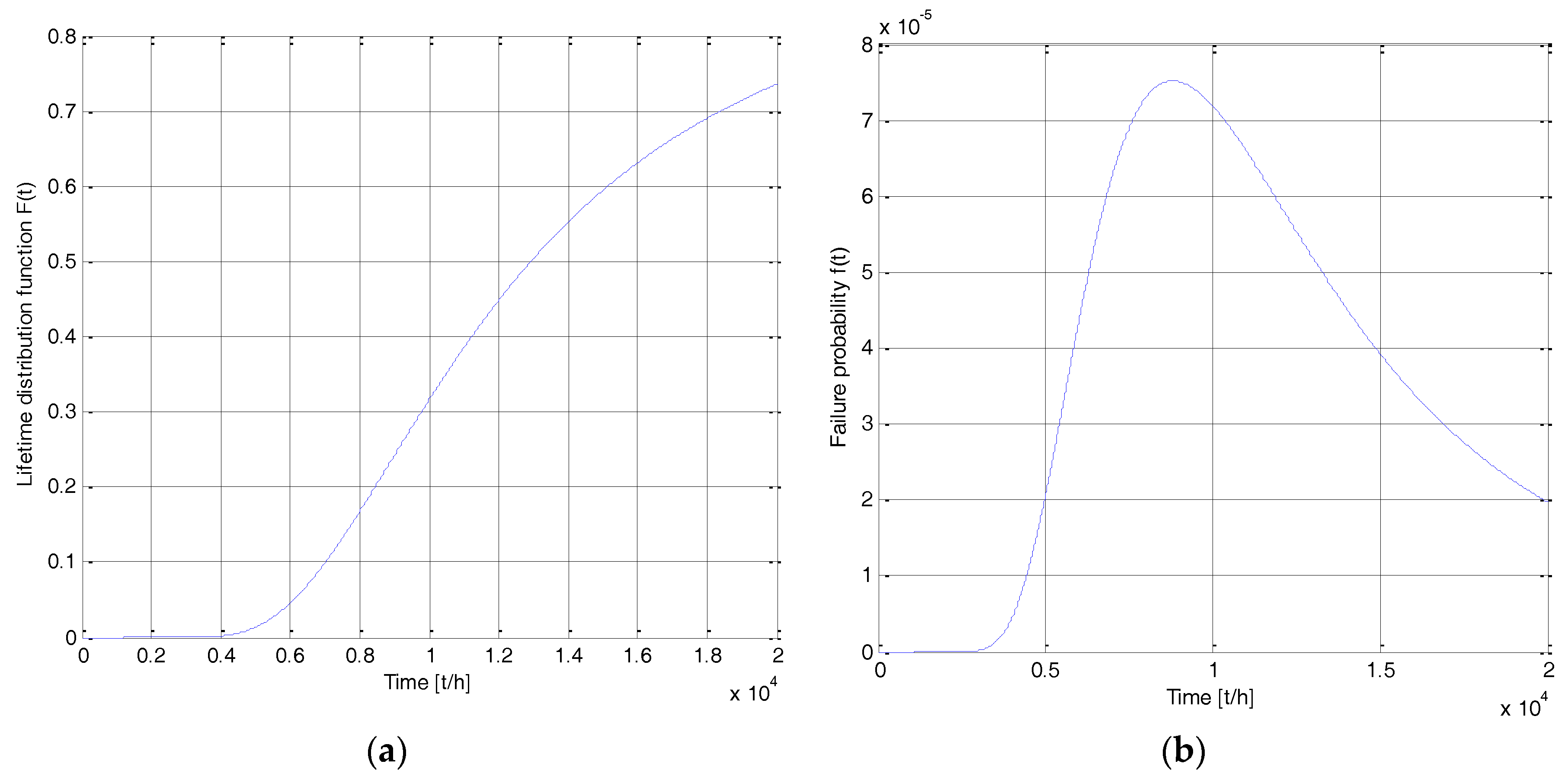
According to the requirements of the bearing design index, the bearing is regarded as a failure when the bearing temperature is 40° higher than the ambient temperature. That is, the failure threshold of the bearing relative temperature is 40°. Therefore, substituting the estimate of the above parameters and the failure threshold in Equations (5), (6), and (16), we get the distribution function, the PDF, and the reliability function of the bearing life shown in Figure 3.

A railway bearing bench test demands 800,000 km equivalent mileage, and the loading test demands a possible reach of 1 million km and a potential speed higher than 200 km/h [16]. Thus, the loading test should not be less than 3333.3 h, and reliability should not be less than 99% for a train speed of 300 km/h.

In Figure 4, we can clearly observe that Curve 2 is more consistent with the actual situation than Curve 1, which is obtained from the literature [17]. The reliability of the test bearings is very high, almost 100%, within 4000 h. At the same time, after the bearing works for 6000 h, with the continual wear and tear of bearing operation, the reliability decline gradually increases. This result basically meets the request of the tested bearings installed in the train, whose highest speed is 200 km/h. However, the observation data was only recorded for 12 h, which is not enough to evaluate reliability, so there is a small gap between the results attained above and the information provided by the manufacturer. Therefore, in order to better evaluate bearing reliability, we still need a long test period to make necessary corrections to reliability evaluation results.

5. Conclusions

Compared with the traditional method based on failure data, performance degradation data can be measured real time during bearing operation, and the results of the reliability analysis can be further revised as the test continues. To avoid additional testing, more sufficient reliability information is necessary. Moreover, differences in product performance may be caused by differences in processing technology, manufacturing errors, and assembling technology in batch production. Therefore, in order to forecast the life of different products and determine general characteristics, we take the unknown coefficients in the model as random variables, so that the model can take the differences between individuals into account and avoid any reduction in the accuracy of reliability assessment.

Future work may aim to study multiple performance degradation indices to improve the efficiency of reliability assessment, since a single performance index generally requires a longer test time.

References

- Si, X.; Wang, W.; Hu, C.; Zhou, D. Estimating remaining useful life with three-source variability in degradation modeling. IEEE Trans. Reliab. 2014, 63, 167–190. [Google Scholar] [CrossRef]
- Jiang, X.; Liu, H.; Zi, J.; Liu, J. Extremely small sample’s reliability of motorized spindle based on Bayes method. J. Vib. Shock 2015, 34, 121–127. [Google Scholar]
- Cai, Z.; Chen, Y.; Li, S.; Wang, Z. Residual Lifetime Prediction Method with Random Degradation and Information Fusion. J. Shanghai Jiao Tong Univ. 2016, 50, 1778–1783. [Google Scholar]
- Zhang, Z.; Si, X.; Hu, C.; Pecht, M. A Prognostic Model for Stochastic Degrading Systems with State Recovery: Application to Li-Ion Batteries. IEEE Trans. Reliab. 2017, 66, 1293–1308. [Google Scholar] [CrossRef]
- Zheng, J.; Hu, C.; Si, X.; Zhang, X. Remaining Useful Life Estimation for Nonlinear Stochastic Degrading Systems with Uncertain Measurement and Unit-to-unit Variability. Acta Autom. Sin. 2017, 43, 259–270. [Google Scholar]
- Pan, Z.; Balakrishnan, N. Multiple-steps step-stress accelerated degradation modeling based on Wiener and gamma processes. Commun. Stat. Simul. Comput. 2010, 39, 1384–1402. [Google Scholar] [CrossRef]
- Pan, Z.; Balakrishnan, N.; Sun, N. Bivariate degradation analysis of products based on Wiener processes and copulas. J. Stat. Comput. Simul. 2013, 83, 1316–1329. [Google Scholar] [CrossRef]
- Pan, Z.; Zhou, J.; Peng, B. Optimal design for accelerated degradation tests with several stresses based on Wiener process. Syst. Eng. Theory Pract. 2009, 29, 64–71. [Google Scholar] [CrossRef]
- Wang, H.; Xu, T.; Mi, Q. Lifetime prediction based on Gamma processes from accelerated degradation data. Chin. J. Aeronaut. 2015, 28, 172–179. [Google Scholar] [CrossRef]
- Tsai, C.C.; Tseng, S.T.; Balakrishnan, N. Optimal design for degradation tests based on Gamma processes with random effects. IEEE Trans. Reliab. 2012, 61, 604–613. [Google Scholar] [CrossRef]
- Lee, M.L.T.; Whitmore, G.A. Threshold regression for survival analysis: Modeling event times by a stochastic process reaching a boundary. Stat. Sci. 2006, 21, 501–513. [Google Scholar] [CrossRef]
- Tsai, C.C.; Tseng, S.T.; Balakrishnan, N. Mis-specification analyses of Gamma and Wiener degradation processes. J. Stat. Plan. Inference 2011, 141, 3725–3735. [Google Scholar] [CrossRef]
- Kim, Y.S.; Sung, S. Practical lifetime estimation strategy based on partially step-stress-accelerated degradation tests. Proc. Instit. Mech. Eng. J. Risk Reliab. 2017, 231, 605–614. [Google Scholar] [CrossRef]
- Balka, J.; Desmond, A.F.; McNicholas, P.D. Review and implementation of cure models based on first hitting times for Wiener Processes. Lifetime Data Anal. 2009, 15, 147–176. [Google Scholar] [CrossRef] [PubMed]
- Chikkara, R.S.; Folks, J.L. The Inverse Gaussian Distribution; Marcell Dekker: New York, NY, USA, 1989. [Google Scholar]
- Yang, X. Overview of High Speed Rail Bearings. Bearings 2011, 10, 59–61. [Google Scholar]
- Zhu, D.; Liu, H.; Yuan, D. Time determination and life assessment of high-speed railway bearing reliability test. China Mech. Eng. 2014, 25, 2886–2891. [Google Scholar]
Figure 1.
The changed tendency of the bearing’s relative temperature.
Figure 2.
Processed bearing performance degradation data.
Figure 3.
(a) Distribution function of bearing life; (b) probability density function (PDF) of bearing life.
Figure 4.
Reliability function of bearing life.
© 2018 by the authors. Licensee MDPI, Basel, Switzerland. This article is an open access article distributed under the terms and conditions of the Creative Commons Attribution (CC BY) license (http://creativecommons.org/licenses/by/4.0/).
Share and Cite
MDPI and ACS Style
Zhu, D.; Nan, C. Reliability Analysis of the High-speed Train Bearing Based on Wiener Process. Information 2018, 9, 15. https://doi.org/10.3390/info9010015
AMA Style
Zhu D, Nan C. Reliability Analysis of the High-speed Train Bearing Based on Wiener Process. Information. 2018; 9(1):15. https://doi.org/10.3390/info9010015
Chicago/Turabian StyleZhu, Dexin, and Cui Nan. 2018. "Reliability Analysis of the High-speed Train Bearing Based on Wiener Process" Information 9, no. 1: 15. https://doi.org/10.3390/info9010015
Note that from the first issue of 2016, this journal uses article numbers instead of page numbers. See further details here.