Gene Selection for Microarray Cancer Data Classification by a Novel Rule-Based Algorithm


Graduate School of Applied Informatics, University of Hyogo, Computational Science Center Building 5-7F, 7-1-28 Minatojima-minamimachi, Chuo-ku, Kobe, Hyogo 650-0047, Japan
Information 2018, 9(1), 6; https://doi.org/10.3390/info9010006
Submission received: 31 October 2017
/
Revised: 26 December 2017
/
Accepted: 27 December 2017
/
Published: 2 January 2018
(This article belongs to the Special Issue Feature Selection for High-Dimensional Data)
Abstract
:Due to the disproportionate difference between the number of genes and samples, microarray data analysis is considered an extremely difficult task in sample classification. Feature selection mitigates this problem by removing irrelevant and redundant genes from data. In this paper, we propose a new methodology for feature selection that aims to detect relevant, non-redundant and interacting genes by analysing the feature value space instead of the feature space. Following this methodology, we also propose a new feature selection algorithm, namely Pavicd (Probabilistic Attribute-Value for Class Distinction). Experiments in fourteen microarray cancer datasets reveal that Pavicd obtains the best performance in terms of running time and classification accuracy when using Ripper-k and C4.5 as classifiers. When using SVM (Support Vector Machine), the Gbc (Genetic Bee Colony) wrapper algorithm gets the best results. However, Pavicd is significantly faster.
1. Introduction
Microarray is a multiplex technology used in molecular biology and medicine that enables biologists to monitor expression levels of thousands of genes [1]. Many microarray experiments have been designed to investigate the genetic mechanisms of cancer [2] and to discover new drug designs in the pharmaceutical industry [3]. According to the World Health Organization, cancer is among the leading causes of death worldwide accounting for more than 8 million deaths. Therefore, finding a mechanism to discover the genetic expressions that may lead to an abnormal growth of cells is a first order task today. To build a microarray, short sequences of genes tagged with fluorescent materials are printed on a glass surface for hibridization [4]. Then, the slice is scanned and goes through various data processing steps including image data collection, quality control and normalization. The resulting dataset is a two-dimensional array with thousands of columns (genes) and several rows (instances):
Every instance (a row in D) is described by a row vector that represents a labeled genetic expression: refers to the expression level of gene , and is the classification for the j-th sample. C may represent different types of cancer or a binary label for cancerous and non-cancerous tissue.
Analysis of microarray data presents unprecedented opportunities and challenges for data mining in areas such as: sample classification and gene selection [5,6]. For sample classification, the microarray matrices serve as training sets to a given classifier, to find a classification function that is able to classify an arbitrary sequence of genes with unknown class from . Classification function ℓ is built from analysing the relation between labeled sequence of genes in D. The performance of supervised classifiers is often measured in three directions: efficiency, representation complexity and accuracy. The efficiency refers to the time required to learn the classification function ℓ, while the representation complexity often refers to the number of bits used to represent the classification function [7]. One of the most common metrics to measure the accuracy of a supervised classifier is the error rate defined as:
where m is the number of sequence of genes in and is the complement of the Kronecker’s delta function, which returns 0 if both arguments are equal and 1 otherwise.
The main obstacle in microarray datasets arises from the fact that the genes greatly outnumber the sample observations. As a popular example, in the “Leukemia” dataset, there are only 72 observations of the expression level of 7129 genes [8]. It is clear that, in this extreme scenario sample, classification methods cannot perform well because of the “curse of dimensionality” phenomena, where excessive features may actually degrade the performance of a classifier if the number of training examples used to build the classifier is relatively small compared to the number of features [7].
Feature selection plays an essential role in microarray data classification since its main goal is to identify and remove irrelevant and redundant genes that do not contribute to minimize the error of a given classifier [9]. Basically, the advantages of feature selection include selecting a set of genes with:
where is the result of projecting over D. In addition, when a small number of genes are selected, their biological relationship with the target diseases is more easily identified. These “marker” genes thus provide additional scientific understanding of the causes of the disease [6]. Feature selection plays a fundamental role for increasing efficiency and enhancing the comprehensibility of the results.
In gene selection, genes are evaluated based on (i) their individual relevance to the target class, (ii) the redundancy level respect to other genes, and (iii) how the gene interacts to other genes [10]. The relevance and the redundancy level of a gene are often measured by correlation coefficients such as: Pearson’s correlation [11], Mutual Information (MI) [12], Symmetrical Uncertainty [13] and others. On the other hand, it is said that a gene interacts with other genes if, when combined, it becomes more relevant [14]. Most of the feature selection algorithms in the literature evaluate features by only using one or two of these aspects, but not using all three of them as a whole. This may lead the algorithm to output low-quality solutions, especially when redundant genes and interacting genes are abundant in the problem. In addition, we have detected that most of feature selection algorithms in the literature suffer from what we call the integrality problem (to be defined). Roughly speaking, the integrality problem occurs when the relevance of a gene is measured by the average of the correlation of their values with the target class. We will further analyse this problem in Section 3.
While not losing sight of the fact that microarray cancer datasets are large and abundant in “noisy” genes, the first goal of this paper is to present a new algorithm able to efficiently detect and select relevant, non-redundant and interacting genes to improve the accuracy of classification algorithms. In order to reach this task:
- We first introduce a new feature selection methodology that can avoid the integrality problem.
- Second, we present a new simple algorithm that can detect irrelevant, redundant and interacting genes in an efficient way.
- Finally, the new algorithm is compared with five state-of-the-art feature selection algorithms in fourteen microarray datasets, which include leukemia, ovarian, lymphoma, breast and other cancer data.
2. Feature Selection for Microarray Cancer Data
Feature selection can be accomplished in a variety of ways depending on the characteristics of the data. In this section, we review most popular algorithms used in microarray cancer data, taking into account two basic group of algorithms: gene ranking and pairwise evaluation methods.
2.1. Gene Ranking Methods
In order to find the optimal subset of features that maximize some feature selection criterion function, an exhaustive search is required, which is a classic NP (non-polynomial) hard problem. Various heuristics and greedy algorithms have been proposed to find suboptimal solutions. The individual relevance score of a gene is a common term that refers to the power of a single gene to predict the class feature C. Assuming independence between genes, the individual relevance score can be used as a metric to select the genes that better predict the class (target disease or phenotype) under certain thresholds. That is, genes are ranked using their individual relevance score and then the top genes are selected. These algorithms are called gene ranking methods and often use correlation, distance and information measures between a single gene and the target class to find genes with high discriminatory power among diseases or phenotypes.
As an instance, the Recursive Feature Elimination algorithm evaluates a gene by computing the added error when is removed from the current set [15]:
where returns the class corresponding to the instance . is the optimal weight of the k-th instance, which is computed with a linear discriminatory classifier such as the Support Vector Machine (Svm). Different from most of the gene ranking algorithms, in the Recursive Feature Elimination approach, a greedy search is performed to add at the end of the ranking the gene that minimize . Although this atypical way of building a ranking leads to a relatively high computational complexity, the quality of the output is high [15]. Fisher Score [16] is a distance-based gene ranking algorithm. Let be the number of instances with class c and let and be the mean and variance of the -th value of all instances in the data, respectively. The Fisher Score represents the average of the distances among instances with different classes when the data are projected with the gene . The Fisher score metric is defined as follows:
Another example is Relief [17], which computes the relevance score of a gene based on the capability of to discriminate among instances of different classes. Assuming instance with class is randomly sampled from the data, and and are two sets of instances (in the neighborhood of ) with class and , respectively, then a gene has high separability power if it has similar values (expression) in instances from and different values in instances from . ReliefF is an extension of Relief that handles multiple classes by splitting the data into series of two-class data [18]. The individual relevance of each gene is assessed by computing the average of its separability power in l instances randomly sampled. That is,
where is the probability that an instance is labeled with class c and , with and being the maximum and minimum value of gene .
It is well known that the assumption of independence between genes leads to the selection of redundant genes and over simplifies the complex relationship between genes [19]. Genes are well known to interact with each other [20]. Several recent research papers on feature selection, especially gene selection [19,21,22], took into consideration the correlation between genes explicitly by genes’ pairwise evaluation.
2.2. Pairwise Evaluation Methods
Oppositely to the gene ranking algorithms, pairwise evaluation algorithms are able to remove redundant genes. The way most of these algorithms operate is as follows. First, the relevance score of each gene is computed, and, second, pairwise evaluations between genes are performed to detect genes that are highly correlated to others (redundant genes). Finally, following some criteria, only relevant and non-redundant genes are selected. As an example, the algorithm Fcbf (Fast Correlation based-Filter) [23] first ranks all genes in the descending order of the Symmetrical Uncertainty scores. Then, starting from the best/first gene in the ranking (with ), it applies a redundancy filter to all of the genes with as follows. If holds, then gene is removed. Since the overall complexity of algorithm Fcbf is , where m is the number of instances in the data, this algorithm is scalable to large microarray data.
Cfs(Correlation-based Feature Selection) is one of the most well-known feature selection algorithms that take advantage of a redundancy filter [24]. Cfs use a Sequential Forward Search to generate candidate sets. Every candidate set is heuristically evaluated as follows:
where represents the average of the relevance score of each gene in and is the average of the redundancy score of all possible pair of genes in . Finally, from all the candidate sets, the one with higher Cfs() value is selected. The time complexity of this algorithm is quadratic in terms of number of genes. Therefore, Cfs is not recommended for high-dimensional microarray data classification problems.
The Minimum Relevance Maximum Relevance (mRMR) algorithm uses a very similar process to select sets of genes [22]. In each iteration, the gene that optimizes certain evaluation functions is selected. Again, the evaluation function corresponds to a balance between the averages of the relevance score and redundancy score of the set of genes already selected :
Assuming that the optimal number of features is not known a priori, one of the disadvantages of mRMR is that the number of features to select must be specified.
Genetic Bee Colony (Gbc) [25] is a well known algorithm in the field of microarray data analysis. Gbc combines the advantages of two naturally inspired algorithms: Genetic Algorithm and Artificial Bee Colony. Since evolutionary algorithms are time-consuming, in Gbc algorithm, the search space is drastically reduced in the first step by discarding the features eliminated by mRmr. In the reduced dataset, Artificial Bee Colony for feature selection is then run with additional crossover and mutation operations, borrowed from Genetic Algorithms, to enhance the exploration process. Although this algorithm is not so fast, it can have a high accuracy since a Support Vector Machine algorithm is used to evaluate the candidate sets by cross validation.
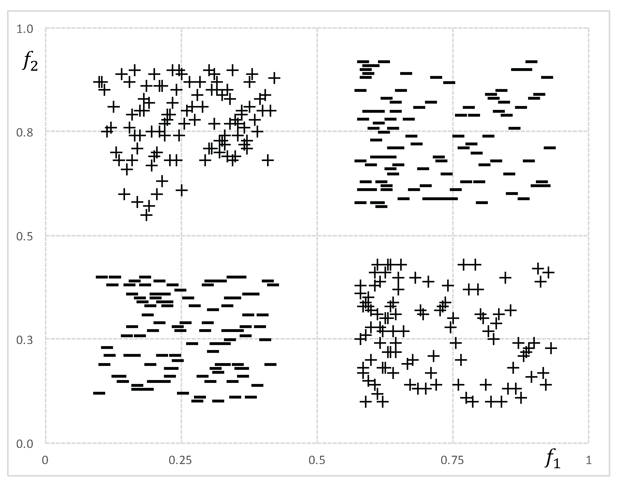
Although feature ranking and pairwise evaluation methods are quite fast and easy to implement, they are not able to detect complex relations among genes. This is why, in high-dimensional microarray data, they may output low-quality sets. To illustrate, consider the class target function where are binary genes and ⊕ denotes the xor operator. Beforehand, we may expect that won’t be selected because both genes by themselves are uncorrelated with c. If we consider that genes in can not accurately describe the class, then we can not expect a good performance of the classifier after reducing F by any of the feature ranking or pairwise evaluation algorithms. Figure 1 depicts a numerical version of the aforementioned example.
The main motivation of this paper is to present an efficient gene selection algorithm able to detect complex relation among relevant genes that yields a significant improvement in the sample classification problem. In the next section, we present a novel methodology for gene selection and a new algorithm derived from such methodology.
3. Materials and Methods
In this section, we introduce a new methodology to create feature selection algorithms that take advantage of feature value information to avoid the integrality problem mentioned in Section 1. For a better understanding of the integrality problem, consider the dataset depicted in Figure 2.
Note that the Symmetrical Uncertainty of , , and with respect to class C is , , and respectively. Therefore, most of the feature selection algorithms described in Section 2, will select as the best feature, and the rest of the features might be selected or not according to their correlation (redundancy score) with . However, it is clear that class C is perfectly predictable by three one-precedent rules when is selected.
This problem occurs because features in have at least one value that is highly correlated with a class label and its other values are not correlated with the class. Consequently, if the relevance of these features (genes) is measured by averaging the prediction power of all its feature values, then this feature may be considered irrelevant. We call this phenomena the integrality problem. Note that we call the correlation of a feature value with respect to a class label of C, to the existing correlation between the binary feature obtained from the respective feature and a given class label. As an example, the feature value of feature is . Note that the correlation between and the target class C, given that , is maximal.
3.1. New Methodology for the Gene Selection Problem
Several feature selection methodologies have been proposed in the literature [9,23]. However, the methodology we introduce in this section is designed so that the search is performed over the expressions of genes (feature values) and not over genes (features). For simplicity, from now on, we refer to an expression of a gene as a feature value, and we refer to a gene as a feature.
As stated above, when a feature has only a feature value that is highly correlated with a class label, then the average of the relevance of all the feature values may be small. Consequently, this feature is often removed by most of the current feature selection algorithms, leading to the loss of important information to predict certain class labels. In order to avoid the integrality problem, our methodology is as follows:
- First, for each class label the feature values that are highly correlated with the class label (according to some evaluation function) are stored in . Optionally, a filter process may be carried out, by eliminating feature values in , whose correlation score does not exceed a certain threshold. From now on, we call this step the Relevance Analysis. Note that is a cluster of feature values with the highest correlation score with respect to .
- Second, feature values in are evaluated/tested among them to determine their redundancy and interaction level. Feature values that are redundant and do not interact with other feature values are removed from . From now on, we call this step the Integration Analysis.
- Third, the set of features that correspond to the feature values in each is returned as the solution.
This methodology is very simple and easy to reproduce. The only entries required are: an evaluation function (that estimates how good an individual feature value is to predict a class label) and a threshold for the Relevance Analysis; and an evaluation function (to measure how good two or more feature values are to predict a class label) for the Integration Analysis. However, the main property that distinguishes this methodology from other feature selection algorithms relies on the fact that the selection process is carried out over the feature value space and not over the feature space. This property may enhance the quality of the feature selection process because features are discriminated according to their contribution to predict only one class label and they are not forced to contain all the necessary information to predict the entire set of class labels, in order to be classified as “good” features. The methodology is depicted in Figure 3.
3.2. Pavicd: A Probabilistic Rule-Based Algorithm
We now introduce a new algorithm, namely Pavicd (Probabilistic Attribute-Value Integration for Class Distinction), which is based on the methodology aforementioned. In order to develop the algorithm, we take into account three aspects: first, how to deal with non-binary datasets, second, how to build for each class label , and third, to develop functions to measure the relevance, redundancy and interaction score of feature values.
The first step in Pavicd is the preparation of data. Since the proposed methodology is based on the evaluation of feature values, instead of features, dealing with non-binary data can be difficult. However, to deal with non-binary data, Pavicd builds a new space of binary features through the decomposition of each feature in (v number of feature values of ) new binary features where each one of them take value “1” in the position, where the respective feature value appears in the original feature and takes value “0” in the other positions. Note that this conversion is reversible because the original feature could be obtained through the union of its binary features. With this transformation, a feature is analysed piecemeal, so that its most intrinsic useful information to predict a given class label is easily identified.
The second step is to determine, and store in which of the entire sets of feature values are relevant for a given class label . Here, we adopt a very simple approach that consists of selecting the covering or reliable feature values for a given class label . Note that we use two thresholds, namely and , to fix the lower bound value for the selection of covering and reliable values, respectively.
Definition 1.
A feature value is said to be covering with respect to the class label if and .
Definition 1 suggests that a feature value is covering with respect to the class if the conditional probability of given is the largest among all the class labels in C. Note that all features values in are covering for at least one class label. Therefore, we use the threshold to discriminate between “good” covering values and "bad" covering values for a given class label.
Definition 2.
A feature value is said to be reliable with respect to the class label if and .
According to Definition 2, a feature value is likely to be reliable for a given class if it occurs many times in and almost does not occur in the rest of the class labels. Note that, again, we introduce a new threshold to filter the feature values.
In the third step, we carried out the Integration Analysis by means of a sequential forward search. The sequential forward search is twofold. First, the best feature value in is identified and included in the current solution set ; and second, the sequential forward search itself is performed. To select the best feature value in , we use the following evaluation function:
This measure is equal to 1 when completely covers and does not occur in any other instance with different class (as feature values , and in the example of Figure 2), and it takes value 0 if the feature value does not occur in any of the instances labelled with class . In other words, we may expect that the best feature value is a highly-covering and highly-reliable one. For the sequential forward search, we start with equal to the feature value in that maximizes Equation (7), and, then, in each iteration, we explore so that feature value that maximizes is selected, and feature value such that holds, is removed from and never tested again. Note that, since Pavicd deals with binary features (or feature values), the current solution is also a binary feature because it is the result of one of “AND” or “OR” operators between two binary features. This is briefly explained below.
To evaluate how good a feature value is with respect to the already selected set , we use the following set of rules:
- Rule 1. If both and are covering feature values, then
- Rule 2. If both and are reliable feature values, then
- Rule 3. If neither Rule 1 or Rule 2 hold, then apply the Rule (1 or 2) that maximizes .
Note that is treated as a feature value (or a binary feature) because every time a feature value is “added” to , is transformed to or if Rule 1 or Rule 2 holds, respectively. Algorithm 1 shows the pseudo code of Pavicd.
| Algorithm 1: Algorithm of Pavicd |
 |
3.3. Complexity Analysis
The first part of Pavicd has a linear time complexity with respect to the number of features n. In this step, instead of computing the mean relevance of each feature as the common feature selection algorithms do, Pavicd analyses all the feature values, which is equivalent in terms of complexity. On the other hand, assuming that each feature has v feature values, the computational complexity in the second step is on average, that is, when the half of the remaining feature values are removed in each iteration.
3.4. Preliminary Evaluation
It is well known that microarray datasets contain interacting genes. In order to test the proposed algorithm, we run some benchmark algorithms in four datasets where the optimal solution is known. Table 1 shows the features selected by each algorithm and the number of errors () for each algorithm. In Table 1—means that a feature that should be selected was not selected, and features in bold letters represent the features that do not belong to the optimal solution.
4. Empirical Study
To evaluate the proposed algorithm, we conduct experiments in fourteen microarray cancer datasets. We compare Pavicd with some of the state-of-the-art feature selection algorithms such as: ReliefF [17], mRMR [22], Fcbf [23], Cfs [24], Interact [26] and Gbc [25]. To run experiments, we implemented mRMR and Gbc algorithms in weka. The rest of the algorithms are available on the weka framework. The experiments were conducted as follows. Given a dataset, we perform the feature selection with all the algorithms listed above to obtain seven reduced datasets, one for each algorithm. At this point, the number of features selected and the running time of each algorithm is compared. To evaluate the accuracy of each algorithm, a ten-fold cross validation is performed over the reduced sets, using four different classifiers: Support Vector Machine (SVM) [27], C4.5 [28], Ripper-k [29] and Naïve Bayes [30]. Classification accuracy is computed and then compared. The classification accuracy depends on the number of instances correctly classified t (true positive + true negative) and is computed by the following formula:
where m is the number of instances of the dataset.
As a final step, non-parametric statistical tests are performed to detect significant differences among the feature selection algorithms. The experiment was performed on the machine learning suite, namely weka [31]. When running Pavicd, we fix the parameters to . For the rest of the algorithms, we use the default values for their parameters. For Svm, we use an Rbf (Radial basis function) kernel with and . To evaluate a feature set, the Gbc algorithm requires training and testing the SVM classifier by cross-validation. After running extensive experiments we decided to train and test the SVM using all the instances in the datasets. In our experiments, there was no difference (in the selected set) between this approach and the leave-one-out cross-validation, except for the running time. Table 2 shows the characteristic of each dataset, which can be found in the OpenML machine learning repository [32].
4.1. Accuracy Evaluation
Table 3, Table 4, Table 5 and Table 6 represent the classification accuracy computed for each classifier after their application on the reduced data. Avg. denotes averaged classification accuracy. It can be seen that Pavicd performs consistently better for Ripper-k and C4.5. We attribute this to the fact that Pavicd detects gene interaction while Naïve Bayes assumes independence between genes. For Svm, Pavicd does not perform so well. However, non-parametric tests reveal that there are not significant differences between the best algorithm when using SVM (Gbc) and Pavicd. For Naïve Bayes, Pavicd has comparable results with the other algorithms in all datasets. One interesting thing to notice is that in many cases the best classification results correspond to Naïve Bayes. The best answer we find by investigating the results more deeply is that in these datasets there are a lot of genes highly-correlated with the target class. However, according to the results, Pavicd is able to detect these type of genes, but the interacting genes found by Pavicd may be useless for Naïve Bayes. Table 3, Table 4, Table 5 and Table 6 also show the averaged ranking of the results.
For Ripper-k, Pavicd found the best reduced sets in ten out of fourteen datasets, which is a promising result. For C4.5, Pavicd found the best results for the fifty percentage of datasets. Figure 4 shows the Critical Distance chart. The Critical Distance was computed using Nemenyi’s equation [33] with .
The post hoc Nemenyi test shows significant differences among the algorithms for the four classifiers. For SVM (Figure 4a), Gbc and Pavicd have significant differences with ReliefF and Interact. Moreover, there are not significant diferences among Gbc and Pavicd. For Naïve Bayes (Figure 4b), algorithms Fcbf, Pavicd, Cfs and mRMR have no differences among them. However, Fcbf and Pavicd show significantly better results than ReliefF and Interact. Speaking about Ripper-k (Figure 4d), Pavicd is significantly better with respect to the rest of the algorithms, and the rest of the algorithms do not have significant differences among them. For C4.5 (Figure 4c), Pavicd is significantly better to all of the algorithms except for Interact.
Next, we examine the performance of the algorithms in terms of number of features selected and running time.
4.2. Number of Features Selected and Running Time
The main goal of feature selection is to reduce the data so that machine learning algorithms can improve their performance. Table 7 shows the running time and the number of genes selected by each feature selection algorithm.
Speaking about the number of genes selected, it is clearly revealed that Interact and Gbc select a small number of genes. However, when we look at the performance of Interact in terms of accuracy (see Section 4.1), we reach the conclusion that Interact might be removing genes with important information for classification. The same applies to Gbc in all the classifiers except SVM. Nevertheless, Pavicd selects a similar number of features with respect to Interact and Gbc, but its performance in terms of accuracy is high. Another conclusion to reach is that the algorithms Cfs and ReliefF select a huge number of features with respect to the rest of the algorithms.
Speaking about running time, surprisingly, Pavicd is the fastest in all datasets except in Var, Ecm and Leu. We further investigated this result and realized that Pavicd removes a lot of genes in early iterations. In addition, we tested two types of implementations of Pavicd: (1) without binarizing the genes and (2) with the binarization process mentioned in Section 3.2. With the first implementation, the running time of Pavicd was slightly larger to Fcbf. However, with the binarization process that transforms the gene space in a binary genes space, the algorithm is extremely fast as shown in Table 7. To better understand the trade-off between the efficiency and effectiveness of the algorithms, Figure 5 depicts a visual comparison between these aspects.
In Figure 5, every algorithm is placed according to their averaged ranks for both running time (vertical axis) and classification accuracy (horizontal axis). Again, the Nemenyi test is performed to compute the critical distance () with . The shadowed area represents the region where there are not significant differences between Pavicd and the rest of the algorithms in terms of both the accuracy and running time. In the context of this experiment, and speaking about the balance between the efficiency and accuracy, we reach the conclusion that Pavicd and Fcbf are the best algorithms for Naïve Bayes and C4.5. While Pavicd performs the best for Ripper-k, Gbc obtains the best results for SVM in terms of accuracy, but the running time is very large in the datasets with the largest dimensions.
We also more deeply investigate the statistical significance of the obtained results, specifically, the observed difference of Pavicd from the other benchmark algorithms by conducting the Benjamini–Hochberg (BH) test [34]. The Bh test controls the false discovery rate (FDR) instead of the family wise error rate (FWER). FWER is the probability of rejecting one or more null hypotheses assuming that all of the null hypotheses are true, while FDR is the conditional probability that a null hypothesis is true when the test indicates rejecting the null hypothesis. The inequality implies a test that controls FDR may be less conservative than a test that controls FWER. In our investigation, we run the Bh test on the maximum values across the classifiers. Fcbf, Cfs, mRmr, Gbc and Pavicd form the top group, and the Bh test showed that the difference is not significant. For the maximum values across the classifiers, we can conclude that all of five of these algorithms are comparable with respect to accuracy, while Fcbf and Pavicd are comparable with respect to time efficiency.
5. Conclusions
Due to the intrinsic distribution of the data population of microarray datasets, where genes greatly outnumber the sample observations, feature selection has proven to be a crucial step for further data analysis such as sample classification. In this paper, we propose a new feature selection algorithm based on a novel methodology, which aims to mitigate the integrality problem. The proposed algorithm, Pavicd, works on the space of feature values instead of the features’ space. This gives the algorithm the opportunity to better detect relevant, non-redundant and interacting features. Experiments in fourteen microarray cancer datasets reveal that Pavicd obtains the best performance in terms of running time and classification accuracy when using Ripper-k and C4.5 as classifiers. When using SVM, the Gbc wrapper algorithm gets the best results. However, Pavicd is significantly faster. In future work, we will evaluate the incidence of the parameters and in the algorithm of Pavicd.
Acknowledgments
This work was partially supported by the Grant-in-Aid for Scientific Research (JSPS KAKENHI Grant Number 17H00762) from the Japan Society for the Promotion of Science.
Conflicts of Interest
The author declares no conflict of interest.
References
- Ruskin, H.J. Computational Modeling and Analysis of Microarray Data: New Horizons. Microarrays 2016, 5, 26. [Google Scholar] [CrossRef] [PubMed]
- Wojtas, B.; Pfeifer, A.; Oczko-Wojciechowska, M.; Krajewska, J.; Czarniecka, A.; Kukulska, A.; Eszlinger, M.; Musholt, T.; Stokowy, T.; Swierniak, M.; et al. Gene Expression (mRNA) Markers for Differentiating between Malignant and Benign Follicular Thyroid Tumours. Int. J. Mol. Sci. 2017, 18, 1184. [Google Scholar] [CrossRef] [PubMed]
- Ferreira, L.G.; dos Santos, R.N.; Oliva, G.; Andricopulo, A.D. Molecular Docking and Structure-Based Drug Design Strategies. Molecules 2015, 20, 13384–13421. [Google Scholar] [CrossRef] [PubMed]
- Hong, H.J.; Koom, W.S.; Koh, W.-G. Cell Microarray Technologies for High-Throughput Cell-Based Biosensors. Sensors 2017, 17, 1293. [Google Scholar] [CrossRef] [PubMed]
- Wang, A.; Gehan, E. Gene selection for microarray data analysis using principle component analysis. Stat. Med. 2005, 24, 2069–2087. [Google Scholar] [CrossRef] [PubMed]
- Zhou, X.; Mao, K. LS bound based gene selection for DNA microarray data. Bioinformatics 2005, 21, 1559–1564. [Google Scholar] [CrossRef] [PubMed]
- Duda, P.; Stork, D.G. Pattern Classification; Wiley-Interscience Publication: Hoboken, NJ, USA, 2001. [Google Scholar]
- Golub, T.; Slonim, D.K.; Tamayo, P.; Huard, C.; Gaasenbeek, M.; Mesirov, J.P.; Coller, H.; Loh, M.L.; Downing, J.R.; Caligiuri, M.A.; et al. Molecular classification of cancer: Class discovery and class prediction by gene expression. Science 1999, 286, 531–537. [Google Scholar] [CrossRef] [PubMed]
- Kohavi, R.; John, G.H. Wrapper for feature subset selection. Artif. Intell. 1997, 97, 273–324. [Google Scholar] [CrossRef]
- Jakulin, A.; Bratko, I. Analyzing attribute dependencies. In Knowledge Discovery in Databases: PKDD; Springer: Berlin, Germany, 2003; pp. 229–240. [Google Scholar]
- Miyahara, K.; Pazzani, M.J. Collaborative filtering with the simple bayesian classifier. In Proceedings of the Pacific Rim International Conference on Artificial Intelligence, Melbourne, Australia, 28 August–1 September 2000; pp. 679–689. [Google Scholar]
- Torkkola, K. Feature extraction by non-parametric mutual information maximization. J. Mach. Learn. Res. 2003, 3, 1415–1438. [Google Scholar]
- Press, W.H.; Flannery, B.P.; Teukolski, S.A.; Vetterling, W.T. Numerical Recipes in C; Cambridge University Press: Cambridge, UK, 1988. [Google Scholar]
- Jakulin, A.; Bratko, I. Quantifying and visualizing attribute interactions: An approach based on entropy. arXiv, 2004; arXiv:cs/0308002v3. [Google Scholar]
- Guyon, I.; Weston, J.; Barnhill, S.; Vapnik, V. Gene Selection for Cancer Classification Using Support Vector Machines. Mach. Learn. 2002, 46, 389–422. [Google Scholar] [CrossRef]
- Gu, Q.; Li, Z.; Han, J. Generalized Fisher score for feature selection. In Proceedings of the Twenty-Seventh Conference on Uncertainty in Artificial Intelligence (UAI’11), Barcelona, Spain, 14–17 July 2011; pp. 266–273. [Google Scholar]
- Kira, K.; Rendell, L.A. A practical approach to feature selection. In Proceedings of the Ninth International Workshop on Machine Learning, Aberdeen, UK, 1–3 July 1992; Morgan Kaufman Publishers Inc.: San Francisco, CA, USA, 1992; pp. 249–256. [Google Scholar]
- Kononenko, I. Estimating attributes: Analysis and extensions of RELIEF. In Proceedings of the European Conference on Machine Learning, Catania, Italy, 6–8 April 1994; pp. 171–182. [Google Scholar]
- Harol, A.; Lai, C.; Pezkalska, E.; Duin, R.P.W. Pairwise feature evaluation for constructing reduced representations. Pattern Anal. Appl. 2007, 10, 55–68. [Google Scholar] [CrossRef]
- Wang, H.; Lo, S.-H.; Zheng, T.; Hu, I. Interaction-based feature selection and classification for high-dimensional biological data. Bioinformatics 2012, 28, 2834–2842. [Google Scholar] [CrossRef] [PubMed]
- Gentile, C. Fast Feature Selection from Microarray Expression Data via Multiplicative Large Margin Algorithms. In Advances in Neural Information Processing Systems 16; MIT Press: Cambridge, MA, USA, 2004; pp. 121–128. [Google Scholar]
- Peng, H.; Long, F.; Ding, C.H.Q. Feature selection based on mutual information: Criteria of max-dependency, max-relevance, and min-redundancy. IEEE Trans. Pattern Anal. Mach. Intell. 2005, 27, 1226–1238. [Google Scholar] [CrossRef] [PubMed]
- Yu, L.; Liu, H. Efficient feature selection via analysis relevance and redundancy. J. Mach. Learn. Res. 2004, 5, 1205–1224. [Google Scholar]
- Hall, M. Correlation-Based Feature Selection for Machine Learning. Ph.D. Thesis, University of Waikato, Hamilton, New Zealand, 2000. [Google Scholar]
- Alshamlan, H.M.; Ghada, H.; Yousef, A. Genetic Bee Colony (GBC) algorithm: A new gene selection method for microarray cancer classification. Comput. Biol. Chem. 2015, 56, 49–60. [Google Scholar] [CrossRef] [PubMed]
- Zhao, Z.; Liu, H. Searching for interacting features. In Proceedings of the IJCAI International Joint Conference on Artificial Intelligence, Hyderabad, India, 6–12 January 2007; pp. 1156–1161. [Google Scholar]
- Ingo, S.; Andreas, C. Support Vector Machines, 1st ed.; Springer: Berlin, Germany, 2008. [Google Scholar]
- Quinlan, J.R. C4.5: Programs for Machine Learning; Morgan Kaufmann Publishers Inc.: San Francisco, CA, USA, 1993. [Google Scholar]
- William, W.C. Fast Effective Rule Induction. In Proceedings of the Twelfth International Conference on Machine Learning, Tahoe City, CA, USA, 9–12 July 1995; pp. 115–123. [Google Scholar]
- Platt, J. Fast Training of Support Vector Machines using Sequential Minimal Optimization. In Advances in Kernel Methods—Support Vector Learning; Schoelkopf, B., Burges, C., Smola, A., Eds.; MIT Press: Cambridge, MA, USA, 1998. [Google Scholar]
- Hall, M.; Frank, E.; Holmes, G.; Pfahringer, B.; Reutemann, P.; Witten, H. The WEKA Data Mining Software: An Update. SIGKDD Explor. 2009, 11, 10–18. [Google Scholar] [CrossRef]
- Vanschoren, J.; Jan, N.; Rijn, V.; Bischl, B.; Torgo, L. OpenML: Networked science in machine learning. SIGKDD Explor. 2013, 15, 49–60. [Google Scholar] [CrossRef]
- Janez, D. Statistical Comparisons of Classifiers over Multiple Data Sets. J. Mach. Learn. Res. 2006, 7, 1–30. [Google Scholar]
- Shaffer, J.P. Multiple hypothesis testing. Ann. Rev. Psychol. 1995, 46, 561–584. [Google Scholar] [CrossRef]
Figure 1.
Numerical features and are represented in a two-dimensional space to demonstrate their interaction to discriminate between class + and class −.
Figure 1.
Numerical features and are represented in a two-dimensional space to demonstrate their interaction to discriminate between class + and class −.

Figure 2.
Dataset with interacting-genes.

Figure 3.
New feature selection methodology, based on the search of feature values, to avoid the integrality problem.
Figure 3.
New feature selection methodology, based on the search of feature values, to avoid the integrality problem.

Figure 4.
Critical Distance charts that show the average ranking of the feature selection algorithms and their significant differences with . (a) Critical Distance chart for SVM; (b) Critical Distance chart for Naïve Bayes; (c) Critical Distance chart for C4.5; (d) Critical Distance chart for Ripper-k.

Figure 5.
Visual comparison of the accuracy and the running time of each algorithm. The figure plots a cross for each algorithm. Each cross is centered on its averaged ranks (for accuracy and running time parameters). The shadowed region represents the area of non-significant difference according to the Nemenyi test with (critical distance is 1.609).


Table 1.
Features selected by some benchmark algorithms in artificial datasets with known solutions.
Table 1.
Features selected by some benchmark algorithms in artificial datasets with known solutions.
| Dataset | Relevant Features | FCBF | Cfs | INTERACT | GBC | PAVICD |
|---|---|---|---|---|---|---|
| Corral | , , , | , , , , | , —, —, —, | , , , | , , , , | , , , |
| Monk1 | , , | , —, , , | —, —, | , , | , , , , | , , |
| Monk2 | , , , , , | —, —, —, , , | —, —, —, , , | , , , , , | , , , , , | , , —, , —, |
| Monk3 | , , | , —, , | , —, | , , , | , , , , | , , |
| #Error | 9 | 10 | 1 | 5 | 3 | |
Table 2.
Datasets used in the experiments.
| Data | Acronym | # Features | # Instances | #Classes | Available at: |
|---|---|---|---|---|---|
| Leukemia | LEU | 7130 | 72 | 2 | https://www.openml.org/d/1104 |
| Anthracycline | ANT | 61,360 | 159 | 2 | https://www.openml.org/d/1085 |
| BreastCancer | BRE | 24,482 | 97 | 2 | http://mldata.org/repository/data/viewslug |
| BurkittLymphoma | BUR | 22,284 | 220 | 3 | https://www.openml.org/d/1084 |
| Central Nervous System | CEN | 7130 | 60 | 2 | http://eps.upo.es/bigs/datasets.html |
| Lymphoma | LYM | 4027 | 96 | 11 | http://eps.upo.es/bigs/datasets.html |
| Difusse B Cell | STAN | 4027 | 47 | 2 | http://eps.upo.es/bigs/datasets.html |
| ECML | ECM | 27,680 | 90 | 43 | http://eps.upo.es/bigs/datasets.html |
| Global Cancer Map | GCM | 16,064 | 144 | 14 | http://eps.upo.es/bigs/datasets.html |
| HepatitisC | HEP | 22,278 | 123 | 4 | https://www.openml.org/search?q=hepatitisC&type=data |
| Leukemia MLL | MLL | 12,583 | 72 | 3 | http://mldata.org/repository/data/viewslug/leukemia-mll/ |
| MouseType | MOU | 45,102 | 214 | 7 | https://www.openml.org/d/1083 |
| Ovarian Cancer | OVA | 54,622 | 283 | 3 | https://www.openml.org/d/1086 |
| Various Cancer | VAR | 54,676 | 383 | 9 | https://www.openml.org/d/1088 |
Table 3.
Classification accuracy with Support Vector Machine.
| Data | LEU | ANT | BRE | BUR | CEN | COM | STAN | ECM | GCM | HEP | MLL | MOU | OVA | VAR | AVG. |
|---|---|---|---|---|---|---|---|---|---|---|---|---|---|---|---|
| SVM | |||||||||||||||
| Fcbf | 100 | 83.6 | 87.4 | 95.5 | 91.7 | 85.7 | 100 | 76.7 | 69.6 | 93.9 | 94.2 | 87.4 | 92.0 | 90.1 | 89.1 |
| RF | 98.6 | 59.7 | 70.2 | 96.0 | 65.0 | 82.4 | 97.3 | 87.8 | 58.5 | 91.0 | 96.7 | 78.4 | 92.2 | 88.4 | 83.0 |
| Cfs | 94.8 | 65.8 | 84.2 | 93.8 | 87.4 | 87.8 | 96.8 | 100 | 63.2 | 93.0 | 97.2 | 72.6 | 94.2 | 98.3 | 87.8 |
| mRMR | 98.6 | 78.0 | 80.1 | 96.0 | 88.3 | 84.3 | 93.2 | 75.6 | 55.6 | 91.8 | 100 | 77.1 | 94.0 | 93.8 | 79.1 |
| INT | 94.3 | 63.5 | 75.2 | 92.3 | 78.3 | 89.2 | 92.9 | 91.1 | 59.0 | 82.9 | 91.7 | 63.6 | 95.4 | 93.9 | 83.1 |
| GBC | 100 | 59.1 | 87.6 | 95.5 | 78.3 | 86.4 | 97.1 | 100 | 86.8 | 96.2 | 97.5 | 57.9 | 95.0 | 97.4 | 87.4 |
| PAV | 95.7 | 66.0 | 84.2 | 96.0 | 83.3 | 86.4 | 97.3 | 89.7 | 64.4 | 94.3 | 97.2 | 74.8 | 94.5 | 94.8 | 86.9 |
| Ranking | |||||||||||||||
| Fcbf | 1.5 | 1.0 | 2.0 | 4.5 | 1.0 | 5.0 | 1.0 | 6.0 | 2.0 | 3.0 | 5.0 | 1.0 | 7.0 | 6.0 | 3.29 |
| RF | 3.5 | 6.0 | 7.0 | 2.0 | 7.0 | 7.0 | 2.5 | 5.0 | 6.0 | 6.0 | 4.0 | 2.0 | 6.0 | 7.0 | 5.07 |
| Cfs | 6.0 | 4.0 | 3.5 | 6.0 | 3.0 | 2.0 | 5.0 | 1.5 | 4.0 | 4.0 | 2.5 | 5.0 | 4.0 | 1.0 | 3.68 |
| mRMR | 3.5 | 2.0 | 5.0 | 2.0 | 2.0 | 6.0 | 6.0 | 7.0 | 7.0 | 5.0 | 7.0 | 3.0 | 5.0 | 5.0 | 4.68 |
| INT | 7.0 | 5.0 | 6.0 | 7.0 | 5.5 | 1.0 | 7.0 | 3.0 | 5.0 | 7.0 | 6.0 | 6.0 | 1.0 | 4.0 | 5.04 |
| GBC | 1.5 | 7.0 | 1.0 | 4.5 | 5.5 | 3.5 | 4.0 | 1.5 | 1.0 | 1.0 | 1.0 | 7.0 | 2.0 | 2.0 | 3.04 |
| PAV | 5.0 | 3.0 | 3.5 | 2.0 | 4.0 | 3.5 | 2.5 | 4.0 | 3.0 | 2.0 | 2.5 | 4.0 | 3.0 | 3.0 | 3.21 |
Table 4.
Classification accuracy with Naïve Bayes.
| Data | LEU | ANT | BRE | BUR | CEN | COM | STAN | ECM | GCM | HEP | LEU | MOU | OVA | VAR | AVG. |
|---|---|---|---|---|---|---|---|---|---|---|---|---|---|---|---|
| Naive Bayes | |||||||||||||||
| Fcbf | 100 | 78.0 | 54.6 | 96.0 | 73.3 | 93.2 | 99.5 | 66.7 | 96.1 | 92.7 | 97.4 | 94.9 | 93.7 | 96.3 | 88.0 |
| RF | 95.8 | 59.7 | 66.0 | 87.7 | 65.0 | 90.9 | 99.2 | 66.7 | 87.6 | 89.4 | 100 | 86.6 | 80.6 | 93.2 | 83.5 |
| Cfs | 96.4 | 77.5 | 76.2 | 92.8 | 71.7 | 92.8 | 99.5 | 69.3 | 96.1 | 87.8 | 93.4 | 93.8 | 93.9 | 95.5 | 88.3 |
| mRMR | 97.2 | 88.7 | 56.7 | 95.0 | 71.7 | 93.4 | 99.5 | 67.2 | 96.1 | 90.2 | 100 | 94.2 | 98.2 | 95.7 | 88.8 |
| INT | 94.4 | 84.0 | 52.6 | 90.0 | 81.7 | 88.7 | 98.9 | 67.1 | 88.1 | 87.8 | 97.4 | 87.1 | 84.3 | 90.0 | 85.2 |
| GBC | 95.8 | 80.2 | 84.5 | 93.6 | 70.0 | 90.2 | 96.4 | 67.0 | 95.2 | 91.9 | 97.4 | 91.0 | 94.2 | 94.1 | 88.7 |
| PAV | 97.2 | 86.9 | 76.2 | 94.1 | 75.0 | 93.9 | 99.3 | 67.2 | 96.3 | 91.9 | 97.4 | 94.9 | 94.5 | 95.6 | 90.0 |
| Ranking | |||||||||||||||
| Fcbf | 1.0 | 5.0 | 6.0 | 1.0 | 3.0 | 3.0 | 2.0 | 6.5 | 3.0 | 1.0 | 4.5 | 1.5 | 5.0 | 1.0 | 3.11 |
| RF | 5.5 | 7.0 | 4.0 | 7.0 | 7.0 | 5.0 | 5.0 | 6.5 | 7.0 | 5.0 | 1.5 | 7.0 | 7.0 | 6.0 | 5.75 |
| Cfs | 4.0 | 6.0 | 2.5 | 5.0 | 4.5 | 4.0 | 2.0 | 1.0 | 3.0 | 6.5 | 7.0 | 4.0 | 4.0 | 4.0 | 4.11 |
| mRMR | 2.5 | 1.0 | 5.0 | 2.0 | 4.5 | 2.0 | 2.0 | 2.5 | 3.0 | 4.0 | 1.5 | 3.0 | 1.0 | 2.0 | 2.57 |
| INT | 7.0 | 3.0 | 7.0 | 6.0 | 1.0 | 7.0 | 6.0 | 4.0 | 6.0 | 6.5 | 4.5 | 6.0 | 6.0 | 7.0 | 5.50 |
| GBC | 5.5 | 4.0 | 1.0 | 4.0 | 6.0 | 6.0 | 7.0 | 5.0 | 5.0 | 2.5 | 4.5 | 5.0 | 3.0 | 5.0 | 4.54 |
| PAV | 2.5 | 2.0 | 2.5 | 3.0 | 2.0 | 1.0 | 4.0 | 2.5 | 1.0 | 2.5 | 4.5 | 1.5 | 2.0 | 3.0 | 2.43 |
Table 5.
Classification accuracy with C4.5.
| Data | LEU | ANT | BRE | BUR | CEN | LYM | DIF | ECM | GCM | HEP | LEU | MOU | OVA | VAR | AVG. |
|---|---|---|---|---|---|---|---|---|---|---|---|---|---|---|---|
| C4.5 | |||||||||||||||
| Fcbf | 80.6 | 68.6 | 67.0 | 78.6 | 68.3 | 92.8 | 68.2 | 76.3 | 78.7 | 87.0 | 97.4 | 81.3 | 70.2 | 86.0 | 78.6 |
| RF | 79.2 | 59.7 | 52.6 | 82.7 | 65.0 | 75.4 | 73.9 | 88.7 | 66.4 | 80.5 | 92.1 | 79.0 | 65.5 | 88.7 | 75.0 |
| Cfs | 85.6 | 70.6 | 81.7 | 85.8 | 69.5 | 73.2 | 87.1 | 88.5 | 78.4 | 84.7 | 95.0 | 85.9 | 71.9 | 81.2 | 81.4 |
| mRMR | 80.6 | 77.4 | 70.1 | 82.7 | 80.0 | 81.9 | 70.2 | 75.5 | 75.2 | 83.7 | 89.5 | 75.1 | 71.6 | 82.9 | 78.3 |
| INT | 90.3 | 78.9 | 73.2 | 87.7 | 76.7 | 83.4 | 85.9 | 72.3 | 77.1 | 80.5 | 97.4 | 84.2 | 74.9 | 83.3 | 81.8 |
| GBC | 84.7 | 73.9 | 68.0 | 85.9 | 72.7 | 81.9 | 83.4 | 91.8 | 77.3 | 88.7 | 81.6 | 84.6 | 66.3 | 81.4 | 80.2 |
| PAV | 87.5 | 71.5 | 82.4 | 87.2 | 73.3 | 82.2 | 87.9 | 88.9 | 78.6 | 86.2 | 97.4 | 86.6 | 78.4 | 90.3 | 84.2 |
| Ranking | |||||||||||||||
| Fcbf | 5.5 | 6.0 | 6.0 | 7.0 | 6.0 | 7.0 | 5.0 | 1.0 | 2.0 | 2.0 | 5.0 | 5.0 | 3.0 | 5.0 | 4.68 |
| RF | 7.0 | 7.0 | 7.0 | 5.5 | 7.0 | 6.0 | 5.0 | 3.0 | 7.0 | 6.5 | 5.0 | 6.0 | 7.0 | 2.0 | 5.79 |
| Cfs | 3.0 | 5.0 | 2.0 | 4.0 | 5.0 | 7.0 | 2.0 | 4.0 | 3.0 | 4.0 | 4.0 | 2.0 | 3.0 | 7.0 | 3.93 |
| mRMR | 5.5 | 2.0 | 4.0 | 5.5 | 1.0 | 4.5 | 6.0 | 6.0 | 6.0 | 5.0 | 6.0 | 7.0 | 4.0 | 5.0 | 4.82 |
| INT | 1.0 | 1.0 | 3.0 | 1.0 | 2.0 | 2.0 | 3.0 | 7.0 | 5.0 | 6.5 | 2.0 | 4.0 | 2.0 | 4.0 | 3.11 |
| GBC | 4.0 | 3.0 | 5.0 | 3.0 | 4.0 | 4.5 | 4.0 | 1.0 | 4.0 | 1.0 | 7.0 | 3.0 | 6.0 | 6.0 | 3.96 |
| PAV | 2.0 | 4.0 | 1.0 | 2.0 | 3.0 | 3.0 | 1.0 | 2.0 | 2.0 | 3.0 | 2.0 | 1.0 | 1.0 | 1.0 | 2.00 |
Table 6.
Classification accuracy with Ripper-k.
| Data | LEU | ANT | BRE | BUR | CEN | COM | STA | ECM | GCM | HEP | LEU | MOU | OVA | VAR | AVG. |
|---|---|---|---|---|---|---|---|---|---|---|---|---|---|---|---|
| Ripper-k | |||||||||||||||
| Fcbf | 84.7 | 59.7 | 75.3 | 83.6 | 71.7 | 79.6 | 87.3 | 89.0 | 77.1 | 82.1 | 97.4 | 82.5 | 86.7 | 83.4 | 81.4 |
| RF | 87.5 | 59.7 | 68.0 | 80.0 | 65.0 | 81.5 | 81.2 | 87.8 | 70.4 | 75.6 | 76.3 | 77.9 | 76.8 | 81.5 | 76.4 |
| Cfs | 91.2 | 67.3 | 77.4 | 83.5 | 76.8 | 77.7 | 92.4 | 87.8 | 81.5 | 86.3 | 95.1 | 84.2 | 74.2 | 86.2 | 83.0 |
| mRMR | 86.1 | 61.6 | 73.2 | 83.2 | 66.7 | 84.3 | 93.7 | 89.8 | 74.8 | 78.0 | 81.6 | 84.1 | 72.9 | 76.9 | 79.1 |
| INT | 94.4 | 67.4 | 74.2 | 86.4 | 75.0 | 79.2 | 89.1 | 89.5 | 74.3 | 78.0 | 97.4 | 77.9 | 75.9 | 81.6 | 81.5 |
| GBC | 87.5 | 63.9 | 63.9 | 86.8 | 65.0 | 84.1 | 94.1 | 90.4 | 76.6 | 82.1 | 84.2 | 82.3 | 70.0 | 76.5 | 79.1 |
| PAV | 91.6 | 69.3 | 79.4 | 86.4 | 80.0 | 85.9 | 89.9 | 89.9 | 83.2 | 90.2 | 97.4 | 84.5 | 87.9 | 87.2 | 85.9 |
| Ranking | |||||||||||||||
| Fcbf | 7.0 | 6.5 | 3.0 | 4.0 | 4.0 | 5.0 | 6.0 | 5.0 | 3.0 | 3.5 | 2.0 | 4.0 | 2.0 | 3.0 | 4.14 |
| RF | 4.5 | 6.5 | 6.0 | 7.0 | 6.5 | 4.0 | 7.0 | 6.5 | 7.0 | 7.0 | 7.0 | 6.5 | 3.0 | 5.0 | 5.96 |
| Cfs | 3.0 | 3.0 | 2.0 | 5.0 | 2.0 | 7.0 | 3.0 | 6.5 | 2.0 | 2.0 | 4.0 | 2.0 | 5.0 | 2.0 | 3.46 |
| mRMR | 6.0 | 5.0 | 5.0 | 6.0 | 5.0 | 2.0 | 2.0 | 3.0 | 5.0 | 5.5 | 6.0 | 3.0 | 6.0 | 6.0 | 4.68 |
| INT | 1.0 | 2.0 | 4.0 | 2.5 | 3.0 | 6.0 | 5.0 | 4.0 | 6.0 | 5.5 | 2.0 | 6.5 | 4.0 | 4.0 | 3.96 |
| GBC | 4.5 | 4.0 | 7.0 | 1.0 | 6.5 | 3.0 | 1.0 | 1.0 | 4.0 | 3.5 | 5.0 | 5.0 | 7.0 | 7.0 | 4.25 |
| PAV | 2.0 | 1.0 | 1.0 | 2.5 | 1.0 | 1.0 | 4.0 | 2.0 | 1.0 | 1.0 | 2.0 | 1.0 | 1.0 | 1.0 | 1.54 |
Table 7.
Running time (in seconds) and number of features selected by the algorithms.
| Running Time (in Seconds) | #Feat. Selected | |||||||||||||
|---|---|---|---|---|---|---|---|---|---|---|---|---|---|---|
| Data | Fcbf | RF | Cfs | mrm | INT | GBC | PAV | Fcbf | RF | Cfs | mrm | INT | GBC | PAV |
| LEU | 1.1 | 0.76 | 206 | 7.49 | 22.1 | 14.5 | 0.79 | 51 | 130 | 51 | 50 | 3 | 5 | 6 |
| ANT | 6.27 | 10.8 | 14763 | 853 | 11653 | 5091 | 4.73 | 67 | 1 | 78 | 50 | 15 | 2 | 29 |
| BRE | 1.81 | 4.8 | 437 | 69.4 | 304 | 321 | 1.28 | 90 | 3 | 89 | 50 | 9 | 5 | 16 |
| BUR | 8.3 | 6.76 | 3215 | 83.1 | 765 | 233 | 3.44 | 208 | 201 | 314 | 50 | 9 | 8 | 27 |
| CEN | 0.27 | 0.52 | 104 | 6.9 | 14.9 | 12.4 | 0.20 | 28 | 1 | 36 | 50 | 8 | 3 | 11 |
| Lym | 0.08 | 0.11 | 501 | 2.9 | 10.6 | 9.7 | 0.07 | 14 | 5 | 154 | 50 | 11 | 3 | 4 |
| STAN | 0.16 | 0.17 | 30 | 2.48 | 4.76 | 7.9 | 0.10 | 60 | 54 | 33 | 50 | 3 | 5 | |
| ECM | 1.81 | 7.26 | 709 | 98.8 | 303 | 572 | 2.23 | 74 | 2750 | 97 | 50 | 7 | 2 | 25 |
| GCM | 4.63 | 5.96 | 428 | 33.3 | 264 | 256 | 3.27 | 67 | 173 | 63 | 50 | 13 | 4 | 37 |
| HEP | 6.73 | 5.13 | 2981 | 57.1 | 485 | 188 | 2.48 | 239 | 626 | 189 | 50 | 6 | 8 | 12 |
| MLL | 2.38 | 1.71 | 1520 | 19.1 | 83.2 | 34.3 | 0.77 | 97 | 580 | 82 | 50 | 3 | 7 | 5 |
| MOU | 11.93 | 10.43 | 5652 | 264 | 2989 | 2739 | 8.32 | 127 | 112 | 233 | 50 | 10 | 4 | 33 |
| OVA | 53.12 | 14.67 | 11412 | 464 | 5849 | 6932 | 9.63 | 734 | 934 | 781 | 50 | 16 | 17 | 13 |
| VAR | 144 | 23.08 | 13902 | 515 | 9920 | 7664 | 37.53 | 934 | 1528 | 827 | 50 | 17 | 19 | 54 |
| AVG. | 17.3 | 6.58 | 3990 | 177 | 2333 | 1720 | 5.35 | 199 | 507 | 216 | 50 | 9.29 | 6.69 | 19.8 |
© 2018 by the author. Licensee MDPI, Basel, Switzerland. This article is an open access article distributed under the terms and conditions of the Creative Commons Attribution (CC BY) license (http://creativecommons.org/licenses/by/4.0/).
Share and Cite
MDPI and ACS Style
Pino Angulo, A. Gene Selection for Microarray Cancer Data Classification by a Novel Rule-Based Algorithm. Information 2018, 9, 6. https://doi.org/10.3390/info9010006
AMA Style
Pino Angulo A. Gene Selection for Microarray Cancer Data Classification by a Novel Rule-Based Algorithm. Information. 2018; 9(1):6. https://doi.org/10.3390/info9010006
Chicago/Turabian StylePino Angulo, Adrian. 2018. "Gene Selection for Microarray Cancer Data Classification by a Novel Rule-Based Algorithm" Information 9, no. 1: 6. https://doi.org/10.3390/info9010006
Note that from the first issue of 2016, this journal uses article numbers instead of page numbers. See further details here.