g-Good-Neighbor Diagnosability of Arrangement Graphs under the PMC Model and MM* Model

Abstract

Diagnosability of a multiprocessor system is an important research topic. The system and interconnection network has a underlying topology, which usually presented by a graph $G=(V,E)$. In 2012, a measurement for fault tolerance of the graph was proposed by Peng et al. This measurement is called the g-good-neighbor diagnosability that restrains every fault-free node to contain at least g fault-free neighbors. Under the PMC model, to diagnose the system, two adjacent nodes in G are can perform tests on each other. Under the MM model, to diagnose the system, a node sends the same task to two of its neighbors, and then compares their responses. The MM* is a special case of the MM model and each node must test its any pair of adjacent nodes of the system. As a famous topology structure, the $(n,k)$-arrangement graph $A_{n,k}$, has many good properties. In this paper, we give the g-good-neighbor diagnosability of $A_{n,k}$ under the PMC model and MM* model.

1. Introduction

A multiprocessor system and interconnection network (networks for short) has an underlying topology, which is usually presented by a graph, where nodes represent processors and links represent communication links between processors. Some processors may fail in the system, so processor fault identification plays an important role for reliable computing. The first step to deal with faults is to identify the faulty processors from the fault-free ones. The identification process is called the diagnosis of the system. A system G is said to be t-diagnosable if all faulty processors can be identified without replacing the faulty processors, provided that the number of faulty processors presented does not exceed t. The diagnosability $t(G)$ of G is the maximum value of t such that G is t-diagnosable [1,2,3]. For a t-diagnosable system, Dahbura and Masson [1] proposed an algorithm with time complex $O(n^{2.5})$, which can effectively identify the set of faulty processors.

Several diagnosis models were proposed to identify the faulty processors. One of most commonly used is the Preparata, Metze, and Chien’s (PMC) diagnosis model introduced by Preparata et al. [4]. The diagnosis of the system is achieved through two linked processors testing each other. A similar issue, namely the comparison diagnosis model (MM model), was proposed by Maeng and Malek [5]. In the MM model, to diagnose the system, a node sends the same task to two of its neighbors, and then compares their responses. The MM* is a special case of the MM model and each node must test its any pair of adjacent nodes of the system.

In 2005, Lai et al. [3] introduced a measurement for fault diagnosis of a system, namely, the conditional diagnosability. They considered the situation that no fault set can contain all the neighbors of any vertex in the system. In 2012, Peng et al. [6] proposed a measurement for fault diagnosis of the system G, namely, the g-good-neighbor diagnosability $t_g(G)$ (which is also called the g-good-neighbor conditional diagnosability), which requires that every fault-free node has at least g fault-free neighbors. In [6], they studied the g-good-neighbor diagnosability of the n-dimensional hypercube under the PMC model. In [7], Wang and Han studied the g-good-neighbor diagnosability of the n-dimensional hypercube under the MM* model. There is a significant amount of research on the g-good-neighbor diagnosability of graphs [6,7,8,9,10,11,12,13,14,15,16,17,18,19,20,21,22,23,24].

The star graph, which was proposed by Akers et al. [25], is a well-known interconnection network. To solve the problem of scalability of star graph topology, Day and Tripathi [26] proposed the arrangement graph as a generalization of the star graph. The arrangement graph $A_{n,k}$ is more flexible than the star graph in selecting the major design parameters: the number, degree, and diameter of the vertex. At the same time, most of the nice properties of the star graph are preserved (for details, see [26,27,28,29,30,31,32]). In this paper, we show (1) $((g+1)(k-2)+2-\lfloor \frac{{(g+1)}^2}{2}\rfloor )(n-k)+g+1\le t_g(A_{n,k})\le [(g+1)(k-1)+1](n-k)$ under the PMC model and MM* model for $n\ge 4$, $k\in [3,n-2],g\in [3,n-k)$; (2) the diagnosability $t(A_{n,k})=k(n-k)$ under the PMC model and MM* model; (3) $t_1(A_{n,k})=(2k-1)(n-k)$ under the PMC model for $n\ge 5$ and $k\in [2,n)$, and under the MM${}^{*}$ model for $n\ge 8$ and $k\in [2,n)$; (4) $t_2(A_{n,k})=(3k-2)(n-k)$ under the PMC model and MM* model for $n\ge 8$ and $k\in [3,n-5]\cup \{n-2,n-1\}$; and (5) $t_2(A_{n,2})=4n-9$ under the PMC model and MM* model for $n\ge 8$.

2. Preliminaries

Under the PMC model [5,23], to diagnose a system $G=(V(G),E(G))$, two adjacent nodes in G can perform tests on each other. For two adjacent nodes u and v in $V(G)$, the test performed by u on v is represented by the ordered pair $(u,v).$ The outcome of a test $(u,v)$ is 1 (respectively, 0) if u evaluate v as faulty (respectively, fault-free). We assume that the test result is reliable (respectively, unreliable) if the node u is fault-free (respectively, faulty). A test assignment T for G is a collection of tests for every adjacent pair of vertices. It can be modeled as a directed testing graph $T=(V(G),L$), where $(u,v)\in L$ implies that u and v are adjacent in G. The collection of all test results for a test assignment T is called a syndrome. Formally, a syndrome is a function $\sigma :L\mapsto \{0,1\}$. The set of all faulty processors in G is called a faulty set. This can be any subset of $V(G)$. For a given syndrome $\sigma$, a subset of vertices $F\subseteq V(G)$ is said to be consistent with $\sigma$ if syndrome $\sigma$ can be produced from the situation that, for any $(u,v)\in L$ such that $u\in V\backslash F$, $\sigma (u,v)=1$ if and only if $v\in F$. This means that F is a possible set of faulty processors. Since a test outcome produced by a faulty processor is unreliable, a given set F of faulty vertices may produce a lot of different syndromes. On the other hand, different faulty sets may produce the same syndrome. Let $\sigma (F)$ denote the set of all syndromes which F is consistent with. Under the PMC model, two distinct sets $F_1$ and $F_2$ in $V(G)$ are said to be indistinguishable if $\sigma (F_1)\cap \sigma (F_2)\ne \mathsf{\varnothing }$; otherwise, $F_1$ and $F_2$ are said to be distinguishable. Besides, we say $(F_1,F_2)$ is an indistinguishable pair if $\sigma (F_1)\cap \sigma (F_2)\ne \mathsf{\varnothing }$; else, $(F_1,F_2)$ is a distinguishable pair.

In the MM model, a processor sends the same task to a pair of distinct neighbors and then compares their responses to diagnose a system G. The comparison scheme of $G=(V(G),E(G))$ is modeled as a multigraph, denoted by $M=(V(G),L)$, where L is the labeled-edge set. A labeled edge ${(u,v)}_w\in L$ represents a comparison in which two vertices u and v are compared by a vertex w, which implies $uw,vw\in E(G)$. We usually assume that the testing result is reliable (respectively, unreliable) if the node u is fault-free (respectively, faulty). If $u,v\in F$ and $w\in V(G)\backslash F$, then ${(u,v)}_w\to 1$. If $u\in F$ and $v,w\in V(G)\backslash F$, then ${(u,v)}_w\to 1$. If $v\in F$ and $u,w\in V(G)\backslash F$, then ${(u,v)}_w\to 1$. If $u,v,w\in V(G)\backslash F$, then ${(u,v)}_w\to 0$. The collection of all comparison results in $M=(V(G),L)$ is called the syndrome of the diagnosis, denoted by $\sigma$. If the comparison ${(u,v)}_w$ disagrees, then $\sigma ({(u,v)}_w)=1$. Otherwise, $\sigma ({(u,v)}_w)=0$. Hence, a syndrome is a function from L to $\{0,1\}$. The MM* is a special case of the MM model and each node must test its any pair of adjacent nodes, i.e., if $uw,vw\in E(G)$, then ${(u,v)}_w\in L$. The set of all faulty processors in the system is called a faulty set. This can be any subset of $V(G)$. For a given syndrome $\sigma$, a faulty subset of vertices $F\subseteq V(G)$ is said to be consistent with $\sigma$ if syndrome $\sigma$ can be produced from the situation that, for any ${(u,v)}_w\in L$ such that $w\in V\backslash F$, $\sigma {(u,v)}_w=1$ if and only if $u,v\in F$ or $u\in F$ or $v\in F$ under the MM${}^{*}$ model. Let $\sigma (F)$ denote the set of all syndromes which F is consistent with. Let $F_1$ and $F_2$ be two distinct faulty sets in $V(G)$. If $\sigma (F_1)\cap \sigma (F_2)\ne \mathsf{\varnothing }$, we say $(F_1,F_2)$ is an indistinguishable pair under the MM${}^{*}$ model; else, $(F_1,F_2)$ is a distinguishable pair under the MM${}^{*}$ model.

Definition 1.

A system $G=(V,E)$ is g-good-neighbor t-diagnosable if $F_1$ and $F_2$ are distinguishable under the PMC (MM${}^{*}$) model for each distinct pair of g-good-neighbor faulty subsets $F_1$ and $F_2$ of V with $|F_1|\le t$ and $|F_2|\le t$. The g-good-neighbor diagnosability $t_g(G)$ of G is the maximum value of t such that G is g-good-neighbor t-diagnosable under the PMC (MM${}^{*}$) model.

A multiprocessor system and network is modeled as an undirected simple graph $G=(V,E)$, whose vertices (nodes) represent processors and edges (links) represent communication links. Given a nonempty vertex subset $V^{\prime }$ of V, the induced subgraph by $V^{\prime }$ in G, denoted by $G\left[V^{\prime }\right]$, is a graph, whose vertex set is $V^{\prime }$ and the edge set is the set of all the edges of G with both endpoints in $V^{\prime }$. For any vertex v, we define the neighborhood $N_G(v)$ of v in G to be the set of vertices adjacent to v. For $u\in N_G(v)$, u is called a neighbor vertex or a neighbor of v. We denote the numbers of vertices and edges in G by $|V(G)|$ and $|E(G)|$. The degree $d_G(v)$ of a vertex v is the number of neighbors of v in G. The minimum degree of a vertex in G is denoted by $\delta (G)$. Let $S\subseteq V$. We use $N_G(S)$ to denote the set ${\cup }_{v\in S}{N}_G(v)\backslash S$. For neighborhoods and degrees, we usually omit the subscript for the graph when no confusion arises. A path in G is a sequence of vertices such that from each of its vertices there is an edge to the next vertex in the sequence. The path with a length of n is denoted by n-path. The length of a shortest path between x and y is called the distance between x and y, denoted by $d_G(x,y)$. A complete graph $K_n$ is a graph in which any two vertices are adjacent on n vertices. A graph $G_1$ is isomorphic to another graph $G_2$ (denoted by $G_1\cong G_2$) if and only if there exists a bijection $\phi :V(G_1)\to V(G_2)$ such that for any two vertices $u,v\in V(G_1)$, $uv\in E(G_1)$ if and only if $\phi (u)\phi (v)\in E(G_2)$. A graph G is said to be k-regular if for any vertex v, $d_G(v)=k$. Let G be connected. The connectivity $\kappa (G)$ of G is the minimum number of vertices whose removal results in a disconnected graph or only one vertex left when G is complete. Let $F_1$ and $F_2$ be two distinct subsets of V, and let the symmetric difference $F_1∆F_2=(F_1\backslash F_2)\cup (F_2\backslash F_1)$. For graph-theoretical terminology and notation not defined here, we follow [33].

Let $G=(V,E)$ be connected. A fault set $F\subseteq V$ is called a g-good-neighbor faulty set if $|N(v)\cap (V\backslash F)|\ge g$ for every vertex v in $V\backslash F$. A g-good-neighbor cut of G is a g-good-neighbor faulty set F such that $G-F$ is disconnected. The minimum cardinality of g-good-neighbor cuts is said to be the g-good-neighbor connectivity of G, denoted by ${\kappa }^{(g)}(G)$. A connected graph G is said to be g-good-neighbor connected if G has a g-good-neighbor cut.

For two positive integers n and k, let $\langle n\rangle$ denote the set $\{1,2,\dots ,n\}$ and $\langle k\rangle$ denote the set $\{1,2,\dots ,k\}$. Let $P_{n,k}$ be a set of arrangements of k elements in $\langle n\rangle$, that is, $P_{n,k}=\{p_1{p}_2\cdots p_k$: $p_i\in \langle n\rangle$ for $1\le i\le k$ and $p_s\ne p_t$ for $1\le s,t\le k$, $s\ne t\}$.

Definition 2.

Given two positive integers n and k with $n>k\ge 1$. The $(n,k)$-arrangement graph, denoted by $A_{n,k}$, has vertex set $V(A_{n,k})=\{p:p=p_1\cdots p_k\in P_{n,k}\}$, and edge set $E(A_{n,k})=\{(p,q):p,q\in V(A_{n,k})$ with $p_i\ne q_i$ for some $i\in \langle k\rangle$ and $p_j=q_j$ for all $j\in \langle k\rangle \backslash \left\{i\right\}\}$.

From the definition, we know that the vertices of $A_{n,k}$ are the arrangements of k elements in $\langle n\rangle$, and the edges of $A_{n,k}$ connect arrangements which differ in exactly one of their k positions. $A_{n,k}$ is a regular graph of degree $k(n-k)$ with $\frac{n!}{(n-k)!}$ vertices. Figure 1 shows the arrangement graph $A_{4,2}$.

Definition 3

([26]). A graph is vertex-transitive if and only if for any pair of its vertices u and v, there exists an automorphism of the graph that maps u to v. A graph is edge-transitive if and only if for any pair of its edges $(u,v)$ and $(x,y)$, there exists an automorphism of the graph that maps $(u,v)$ to $(x,y)$.

Lemma 1

([26]). $A_{n,k}$ is vertex-transitive and edge-transitive.

Lemma 2

([26]). $\kappa (A_{n,k})=k(n-k)$ for $n>k\ge 1$.

Lemma 3

([28]). $n\ge 3$ and $n\ne 4$, $k\in [2,n)$, ${\kappa }^{(1)}(A_{n,k})=(2k-1)(n-k)-1$ and ${\kappa }^{(1)}(A_{4,2})={\kappa }^{(1)}(A_{4,3})(={\kappa }^{(1)}(S_4))=4$.

Lemma 4

([28]). $n\ge 3$ and $n\ne 4$, $2\le k<n$, ${\kappa }^{(1)}(A_{n,k})=(2k-1)(n-k)-1$ and ${\kappa }^{(1)}(A_{4,2})={\kappa }^{(1)}(A_{4,3})(={\kappa }^{(1)}(S_4))=4$.

Lemma 5

([28]). For $n\ge 8$, ${\kappa }^{(2)}(A_{n,2})=4n-12$, and, for $k\in \{i:i=3,\dots ,n-5\}\cup \{n-2,n-1\}$, ${\kappa }^{(2)}(A_{n,k})=(3k-2)(n-k)-2$.

Lemma 6

([28]). Let $n,k,g$ be positive integers such that $n\ge 4$, $2\le k\le n-2,g\ge 3$. Then,

$$((g+1)(k-2)+2-\frac{{(g+1)}^2}{2})(n-k)<{\kappa }^{(g)}(A_{n,k})\le [(g+1)(k-1)+1](n-k)-g.$$

An edge cut of a graph G is a set of edges whose removal makes the remaining graph no longer connected. The edge connectivity $\lambda (G)$ of G is the minimum cardinality of an edge cut of G.

Lemma 7

([33]). $\kappa (G)\le \lambda (G)\le \delta (G)$.

According to Lemmas 2 and 7, we get the following corollary.

Corollary 1.

The edge connectivity $\lambda (A_{n,k})=k(n-k)$ for $n>k\ge 1$.

For $i\in \langle n\rangle$, $j\in \langle k\rangle$, let $V(A_{n,k}^{j:i})$ be the set of all vertices in $A_{n,k}$ with the jth position being i, that is, $V(A_{n,k}^{j:i})=\{p:p=p_1\cdots p_j\cdots p_k\in P_{n,k}$ with $p_j=i\}$. It is easy to check that each $A_{n,k}^{j:i}$ is a subgraph of $A_{n,k}$, and we say that $A_{n,k}$ is decomposed into n subgraphs $A_{n,k}^{j:i}$$(1\le i\le n)$ according to the jth position. For simplicity, we shall take j as the last position k, and use $A_{n,k}^i$ to denote $A_{n,k}^{k:i}$. Then, $V(A_{n,k}^i)=\{p:p=p_1\cdots p_{k-1}i$ with $p_j\in \langle n\rangle \backslash \left\{i\right\}$ and $p_s\ne p_t$ for $1\le s,t\le k-1\}$ for $1\le i\le n$. It is easy to see that $A_{n,1}$ is a complete graph $K_n$.

Proposition 1

([34]). Let $n>k\ge 2$. For each $j\in \langle k\rangle$, $A_{n,k}^{j:i}$ is isomorphic to $A_{n-1,k-1}$ where $1\le i\le n$.

For any vertex $u\in V(A_{n,k}^i)$$(1\le i\le n)$, in this paper, we say that $N(u)\cap V(A_{n,k}^i)$ is the set of inner neighbors of u, which is denoted by $IN(u)$ and $N(u)\cap (V(A_{n,k})\backslash V(A_{n,k}^i))$ is the set of outer neighbors of u, which is denoted by $ON(u)$.

Proposition 2

([31]). Let $n>k\ge 2$, $i\in \langle n\rangle$. For any two vertices u, v in the subgraph $A_{n,k}^i$, $ON(u)\cap ON(v)=\mathsf{\varnothing }$ and $|ON(u)|=n-k$. Furthermore, the vertices of $ON(u)$ are distributed in $(n-k)$ distinct subgraphs.

Proposition 3.

For any vertex $u\in V(A_{n,k}^i)$$(1\le i\le n)$, let $ON(u)$ be the set of outer neighbors of u. Then, $A_{n,k}[\left\{u\right\}\cup ON(u)]$ is isomorphic to the complete graph $K_{n-k+1}$.

Proof. 

By Lemma 1, $A_{n,k}$ is vertex-transitive. Without loss of generality, let $u=(n-k+1)(n-k+2)\cdots n\in V(A_{n,k}^n)$. By the definition of arrangement graphs, $ON(u)=\{u_j:u_j=(n-k+1)(n-k+2)\cdots (n-1)j,j\in \{1,2,\dots ,n-k\}\}$. Then, $|ON(u)|=n-k$. Note that u, $u_1$,…,$u_{n-k-1}$ and $u_{n-k}$ are only different in last position. By the definition of arrangement graphs, any pair of vertices of u $u_1$,…,$u_{n-k-1}$ and $u_{n-k}$ are adjacent. Thus, $A_{n,k}[\left\{u\right\}\cup ON(u)]$ is a complete graph. Note that $|\{u\}\cup ON(u)|=n-k+1$. Thus, $A_{n,k}[\left\{u\right\}\cup ON(u)]$ is isomorphic to $K_{n-k+1}$. □

Definition 4.

Let $\langle n\rangle =\{1,2,\cdots ,n\}$, and let $S_n$ be the symmetric group on $\langle n\rangle$ containing all permutations $p=p_1{p}_2\cdots p_n$ of $\langle n\rangle$. The alternating group $A_n$ is the subgroup of $S_n$ containing all even permutations. It is well known that $\{(12i),(1i2),3\le i\le n\}$ is a generating set for $A_n$. The n-dimensional alternating group graph $A{G}_n$ is the graph with vertex set $V(A{G}_n)$ = $A_n$ in which two vertices u, v are adjacent if and only if $u=v(12i)$ or $u=v(1i2)$, $3\le i\le n$.

Definition 5.

The n-dimensional star graph denoted by $S_n$. The vertex set of $S_n$ is $\{u_1{u}_2\cdots u_n:u_1{u}_2\cdots u_n$ is a permutation of $\langle n\rangle \}$. Vertex adjacency is defined as follows: $u_1{u}_2\cdots u_n$ is adjacent to $u_i{u}_2\cdots u_{i-1}{u}_1{u}_{i+1}\cdots u_n$ for all $2\le i\le n$.

Lemma 8

([29]). (1). The arrangement graph $A_{n,n-2}$ is isomorphic to the n-dimensional alternating group graph $A{G}_n$. (2). The arrangement graph $A_{n,n-1}$ is isomorphic to the n-dimensional star graph $S_n$.

Lemma 9

([31]). For any two distinct vertices u and v in the arrangement graph $A_{n,k}$, we have the following results:

1. 

If $d(u,v)=1$, then $|N(u)\cap N(v)|=n-k-1$;

2. 

If $d(u,v)=2$ and $n=k+1$, then $|N(u)\cap N(v)|=1$;

3. 

If $d(u,v)=2$ and $n\ge k+2$, then $|N(u)\cap N(v)|\le 2$; and

4. 

If $d(u,v)\ge 3$, then $|N(u)\cap N(v)|=0$.

3. The g-Good-Neighbor Diagnosability of Arrangement Graphs under the PMC Model

In this section, we show the g-good-neighbor diagnosability of arrangement graphs under the PMC model (Figure 2).

Theorem 1

([23]). A system $G=(V,E)$ is g-good-neighbor t-diagnosable under the $PMC$ model if and only if there is an edge $uv\in E$ with $u\in V\backslash (F_1\cup F_2)$ and $v\in F_1∆F_2$ for each distinct pair of g-good-neighbor faulty subsets $F_1$ and $F_2$ of V with $|F_1|\le t$ and $|F_2|\le t$.

Lemma 10

([28]). For $n\ge 3$ and $n\ne 4$, $2\le k<n$, ${\kappa }^{(1)}(A_{n,k})=(2k-1)(n-k)-1$ and ${\kappa }^{(1)}(A_{4,2})={\kappa }^{(1)}(A_{4,3})(={\kappa }^{(1)}(S_4))=4$.

Lemma 11

([28]). For $n\ge 8$, ${\kappa }^{(2)}(A_{n,2})=4n-12$, and, for $k\in \{i:i=3,\dots ,n-5\}\cup \{n-2,n-1\}$, ${\kappa }^{(2)}(A_{n,k})=(3k-2)(n-k)-2$.

Lemma 12

([27]). Let $n\ge 7$ and let T be a subset of the vertices of $A_{n,2}$ such that $|T|\le 4n-12$. Then, $A_{n,2}-T$ is either connected or has a large component and small components with at most two vertices or $|T|=4n-12$ and $A_{n,2}-T$ has a large component and a four-cycle.

Lemma 13

([28]). Let $n,k,g$ be positive integers such that $n\ge 4,2\le k\le n-2,3\le g<n-k$. Then,

$$((g+1)(k-2)+2-\frac{{(g+1)}^2}{2})(n-k)<{\kappa }^{(g)}(A_{n,k})\le [(g+1)(k-1)+1](n-k)-g.$$

Let $\alpha \in P(n,k-1)$, $\alpha =p_1\dots p_{k-1}$ and $V_{\alpha }=\{p_1\dots p_{k-1}i:i\in \langle n\rangle \backslash \{p_1,\dots ,p_{k-1}\}\}$. Let $u=\alpha i=p_1\dots p_{k-1}i$ and $v=\alpha j=p_1\dots p_{k-1}j,i\ne j$ and neither i nor j occurs in $\alpha$. Clearly, $u,v\in V(A_{n,k})$, and $(u,v)\in E(A_{n,k})$. Since any symbol that does not occur in $\alpha$ can serve as the last symbol in a vertex in $V_{\alpha }$, $|V_{\alpha }|=n-(k-1)$. Thus, the graph $K_{n+k+1}^{\alpha }$ induced by $V_{\alpha }$ is a complete graph of order $n-k+1$. Let $g\in [0,n-k)$ and $X\subseteq V(K_{n+k+1}^{\alpha })$ such that $|X|=g+1$. Notice that $g+1=|X|<|V(K_{n+k+1}^{\alpha })|=n-k+1$. Then, $A_{n,k}\left[X\right]$ is a complete graph $K_{g+1}$.

Lemma 14.

Let $n,k,g$ be positive integers such that $n\ge 3$, $2\le k<n$, $0\le g<n-k$, and let $A_{n,k}$ be the arrangement graph. Let X be defined as above, and let $F_1=N_{A_{n,k}}(X)$, $F_2=X\cup N_{A_{n,k}}(X)$. Then, $|F_1|=[(g+1)(k-1)+1](n-k)-g$, $|F_2|=[(g+1)(k-1)+1](n-k)+1$, $\delta (A_{n,k}\left[X\right])\ge g$ and $\delta (A_{n,k}-F_1-F_2)\ge g$.

Proof. 

Let X be defined as above. By the process of the proof of Lemma 13 in [28], $N(X)$ is a g-good-neighbor cut of $A_{n,k}$ and $|N(X)|=|F_1|=[(g+1)(k-1)+1](n-k)-g$. Since $|X|=g+1$, $|F_2|=[(g+1)(k-1)+1](n-k)+1$. □

Lemma 15.

Let $n\ge 3$, $2\le k<n$ and $0\le g<n-k$. Then, the g-good-neighbor diagnosability of the arrangement graph $A_{n,k}$ under the PMC model is less than or equal to $[(g+1)(k-1)+1](n-k)$, i.e., $t_g(A_{n,k})\le [(g+1)(k-1)+1](n-k)$.

Proof. 

Let X be defined as above, and let $F_1=N_{A_{n,k}}(X)$, $F_2=X\cup N_{A_{n,k}}(X)$. By Lemma 14, $|F_1|=[(g+1)(k-1)+1](n-k)-g$, $|F_2|=|X|+|F_1|=[(g+1)(k-1)+1](n-k)+1$, $\delta (A_{n,k}-F_1)\ge g$ and $\delta (A_{n,k}-F_2)\ge g$. Therefore, $F_1$ and $F_2$ are g-good-neighbor faulty sets of $A_{n,k}$ with $|F_1|=[(g+1)(k-1)+1](n-k)-g$ and $|F_2|=[(g+1)(k-1)+1](n-k)+1$.

We prove that $A_{n,k}$ is not g-good-neighbor $([(g+1)(k-1)+1](n-k)+1)$-diagnosable. Since $X=F_1∆F_2$ and $N_{A_{n,k}}(X)=F_1\subset F_2$, there is no edge of $A_{n,k}$ between $V(A_{n,k})\backslash (F_1\cup F_2)$ and $F_1∆F_2$. By Theorem 1, we can show that $A_{n,k}$ is not g-good-neighbor $([(g+1)(k-1)+1](n-k)+1)$-diagnosable under the PMC model. Hence, by the definition of the g-good-neighbor diagnosability, we show that the g-good-neighbor diagnosability of $A_{n,k}$ is less than $[(g+1)(k-1)+1](n-k)+1$, i.e., $t_g(A_{n,k})\le [(g+1)(k-1)+1](n-k)$. □

Lemma 16.

Let $n,k,g$ be positive integers such that $n\ge 4$, $2\le k\le n-2,3\le g<n-k$. Then, the arrangement graph $A_{n,k}$ is g-good-neighbor $(((g+1)(k-2)+2-\lfloor \frac{{(g+1)}^2}{2}\rfloor )(n-k)+g+1)$-diagnosable under the PMC model.

Proof. 

By Theorem 1, to prove $A_{n,k}$ is g-good-neighbor $(((g+1)(k-2)+2-\lfloor \frac{{(g+1)}^2}{2}\rfloor )(n-k)+g+1)$-diagnosable, it is equivalent to prove that there is an edge $uv\in E(A_{n,k})$ with $u\in V(A_{n,k})\backslash (F_1\cup F_2)$ and $v\in F_1∆F_2$ for each distinct pair of g-good-neighbor faulty subsets $F_1$ and $F_2$ of $V(A_{n,k})$ with $|F_1|\le ((g+1)(k-2)+2-\lfloor \frac{{(g+1)}^2}{2}\rfloor )(n-k)+g+1$ and $|F_2|\le ((g+1)(k-2)+2-\lfloor \frac{{(g+1)}^2}{2}\rfloor )(n-k)+g+1$.

We prove this statement by contradiction. Suppose that there are two distinct g-good-neighbor faulty subsets $F_1$ and $F_2$ of $A_{n,k}$ with $|F_1|\le ((g+1)(k-2)+2-\lfloor \frac{{(g+1)}^2}{2}\rfloor )(n-k)+g+1$ and $|F_2|\le ((g+1)(k-2)+2-\lfloor \frac{{(g+1)}^2}{2}\rfloor )(n-k)+g+1$, but the vertex set pair $(F_1,F_2)$ is not satisfied with the condition in Theorem 1, i.e., there are no edges between $V(A_{n,k})\backslash (F_1\cup F_2)$ and $F_1∆F_2$. Without loss of generality, suppose that $F_2\backslash F_1\ne \mathsf{\varnothing }$.

Case 1. $V(A_{n,k})=F_1\cup F_2$.

Note that $(g+1)(k-2)+2-\frac{{(g+1)}^2}{2}=-\frac{g^2}{2}+(k-3)g+k-\frac{1}{2}$. Since $k\in [2,n-2]$, $-\frac{g^2}{2}+(k-3)g+k-\frac{1}{2}\le -\frac{g^2}{2}+(n-5)g+n-2-\frac{1}{2}$. Let $y=-\frac{g^2}{2}+(n-5)g+n-2-\frac{1}{2}$. Then, $y_{max}=\frac{1}{2}{n}^2-4n+10$ for $g=n-5$ and $-\frac{g^2}{2}+(k-3)g+k-\frac{1}{2}\le \frac{1}{2}{n}^2-4n+10$.

Assume $V(A_{n,k})=F_1\cup F_2$. We have that $\frac{n!}{(n-k)!}=|V(A_{n,k})|=|F_1\cup F_2|=|F_1|+|F_2|-|F_1\cap F_2|\le |F_1|+|F_2|\le 2(((g+1)(k-2)+2-\lfloor \frac{{(g+1)}^2}{2}\rfloor )(n-k)+g+1)\le 2(((g+1)(k-2)+2-\frac{{(g+1)}^2}{2})(n-k)+g+1)\le 2((\frac{1}{2}{n}^2-4n+10)(n-k)+g+1)=(n^2-8n+20)(n-2)+2(n-2)+2=n^3-10n^2+34n-34$. When $k=3$, $\frac{n!}{(n-k)!}=n^3-3n^2+2n$. Note $n^3-3n^2+2n\le \frac{n!}{(n-k)!}$ for $k\ge 3$. Thus, $n^3-3n^2+2n\le n^3-10n^2+36n-40$. In fact, $n^3-3n^2+2n>n^3-10n^2+36n-40$ when $n\ge 4$. This is a contradiction. Therefore, $V(A_{n,k})\ne F_1\cup F_2$.

Case 2. $V(A_{n,k})\ne F_1\cup F_2$

According to the hypothesis, there are no edges between $V(A_{n,k})\backslash (F_1\cup F_2)$ and $F_1∆F_2$. Since $F_1$ is a g-good-neighbor faulty set and $A_{n,k}-F_1$ has two parts $A_{n,k}-F_1-F_2$ and $A_{n,k}[F_2\backslash F_1]$, we have that $\delta (A_{n,k}-F_1-F_2)\ge g$ and $\delta (A_{n,k}[F_2\backslash F_1])\ge g$. Similarly, $\delta (A_{n,k}[F_1\backslash F_2])\ge g$ when $F_1\backslash F_2\ne \mathsf{\varnothing }$. Therefore, $F_1\cap F_2$ is also a g-good-neighbor faulty set. Since there are no edges between $V(A_{n,k}-F_1-F_2)$ and $F_1∆F_2$, $F_1\cap F_2$ is also a g-good-neighbor cut. When $F_1\backslash F_2=\mathsf{\varnothing }$, $F_1\cap F_2=F_1$ is also a g-good-neighbor faulty set. Since there are no edges between $V(A_{n,k}-F_1-F_2)$ and $F_1∆F_2$, $F_1\cap F_2$ is a g-good-neighbor cut. By Lemma 13, $|F_1\cap F_2|\ge ((g+1)(k-2)+2-\lfloor \frac{{(g+1)}^2}{2}\rfloor )(n-k)+1$. Since $\delta (A_{n,k}[F_2\backslash F_1])\ge g$, $|F_2\backslash F_1|\ge g+1$. Therefore, $|F_2|=|F_2\backslash F_1|+|F_1\cap F_2|\ge g+1+((g+1)(k-2)+2-\lfloor \frac{{(g+1)}^2}{2}\rfloor )(n-k)+1=((g+1)(k-2)+2-\lfloor \frac{{(g+1)}^2}{2}\rfloor )(n-k)+g+2$, which contradicts with that $|F_2|\le ((g+1)(k-2)+2-\lfloor \frac{{(g+1)}^2}{2}\rfloor )(n-k)+g+1$. Thus, $A_{n,k}$ is g-good-neighbor $(((g+1)(k-2)+2-\lfloor \frac{{(g+1)}^2}{2}\rfloor )(n-k)+g+1)$-diagnosable. By the definition of $t_g(A_{n,k})$, $t_g(A_{n,k})\ge ((g+1)(k-2)+2-\lfloor \frac{{(g+1)}^2}{2}\rfloor )(n-k)+g+1$. The proof is complete. □

Combining Lemmas 15 and 16, we have the following theorem.

Theorem 2.

Let $n,k,g$ be positive integers such that $n\ge 4$, $3\le k\le n-2,3\le g<n-k$. Then, $((g+1)(k-2)+2-\lfloor \frac{{(g+1)}^2}{2}\rfloor )(n-k)+g+1\le t_g(A_{n,k})\le [(g+1)(k-1)+1](n-k)$ under the PMC model.

Theorem 3.

Let $A_{n,k}$ be the arrangement graph with $n>k\ge 2$. Then, the diagnosability $t(A_{n,k})=k(n-k)$ under the PMC model.

Proof. 

Let $u\in V(A_{n,k})$. Then, $N(u)$ is a cut of $A_{n,k}$ and $|N(u)|=k(n-k)$. Let $F_1=N(u)$, $F_2=\left\{u\right\}\cup N(u)$. Then, $|F_1|=k(n-k)$, $|F_2|=|X|+|F_1|=k(n-k)+1$, $\delta (A_{n,k}-F_1)\ge 0$ and $\delta (A_{n,k}-F_2)\ge 0$. Therefore, $F_1$ and $F_2$ are 0-good-neighbor faulty sets of $A_{n,k}$ with $|F_1|=k(n-k)$ and $|F_2|=k(n-k)+1$. We will prove $A_{n,k}$ is not 0-good-neighbor $(k(n-k)+1)$-diagnosable. Since $\left\{u\right\}=F_1∆F_2$ and $N(u)=F_1\subset F_2$, there is no edge of $A_{n,k}$ between $V(A_{n,k})\backslash (F_1\cup F_2)$ and $F_1∆F_2$. By Theorem 1, we can show that $A_{n,k}$ is not 0-good-neighbor $(k(n-k)+1)$-diagnosable under the PMC model. Hence, by the definition of the 0-good-neighbor diagnosability, we conclude that the 0-good-neighbor diagnosability of $A_{n,k}$ is less than $k(n-k)+1$, i.e., $t_0(A_{n,k})\le k(n-k)$.

By Theorem 1, to prove $A_{n,k}$ is 0-good-neighbor $k(n-k)$-diagnosable, it is equivalent to prove that there is an edge $uv\in E(A_{n,k})$ with $u\in V(A_{n,k})\backslash (F_1\cup F_2)$ and $v\in F_1∆F_2$ for each distinct pair of 0-good-neighbor faulty subsets $F_1$ and $F_2$ of $V(A_{n,k})$ with $|F_1|\le k(n-k)$ and $|F_2|\le k(n-k)$.

We prove this statement by contradiction. Suppose that there are two distinct 0-good-neighbor faulty subsets $F_1$ and $F_2$ of $A_{n,k}$ with $|F_1|\le k(n-k)$ and $|F_2|\le k(n-k)$, but the vertex set pair $(F_1,F_2)$ is not satisfied with the condition in Theorem 1, i.e., there are no edges between $V(A_{n,k})\backslash (F_1\cup F_2)$ and $F_1∆F_2$. Without loss of generality, suppose that $F_2\backslash F_1\ne \mathsf{\varnothing }$.

Assume $V(A_{n,k})=F_1\cup F_2$. We have that $\frac{n!}{(n-k)!}=|V(A_{n,k})|=|F_1\cup F_2|=|F_1|+|F_2|-|F_1\cap F_2|\le |F_1|+|F_2|\le 2k(n-k)$. When $k=2$, $n^2-n=\frac{n!}{(n-2)!}\le 4n-8$, a contradiction. Therefore, $V(A_{n,2})\ne F_1\cup F_2$. When $k=3$, $\frac{n!}{(n-k)!}=n^3-3n^2+2n$. Note $n^3-3n^2+2n\le \frac{n!}{(n-k)!}$ and $2k(n-k)\le 2n^2-8n+6$ for $k\ge 3$. Thus, $n^3-3n^2+2n\le 2n^2-8n+6$. In fact, $n^3-3n^2+2n>2n^2-8n+6$ when $n\ge 4$. This is a contradiction. Therefore, $V(A_{n,k})\ne F_1\cup F_2$.

According to the hypothesis, there are no edges between $V(A_{n,k})\backslash (F_1\cup F_2)$ and $F_1∆F_2$. Since $F_1$ is a 0-good-neighbor faulty set and $A_{n,k}-F_1$ has two parts $A_{n,k}-F_1-F_2$ and $A_{n,k}[F_2\backslash F_1]$, we have that $\delta (A_{n,k}-F_1-F_2)\ge 0$ and $\delta (A_{n,k}[F_2\backslash F_1])\ge 0$. Similarly, $\delta (A_{n,k}[F_1\backslash F_2])\ge 0$ when $F_1\backslash F_2\ne \mathsf{\varnothing }$. Therefore, $F_1\cap F_2$ is also a 0-good-neighbor faulty set. Since there are no edges between $V(A_{n,k}-F_1-F_2)$ and $F_1∆F_2$, $F_1\cap F_2$ is also a 0-good-neighbor cut. When $F_1\backslash F_2=\mathsf{\varnothing }$, $F_1\cap F_2=F_1$ is also a 0-good-neighbor faulty set. Since there are no edges between $V(A_{n,k}-F_1-F_2)$ and $F_1∆F_2$, $F_1\cap F_2$ is a 0-good-neighbor cut. By Lemma 2, $|F_1\cap F_2|\ge k(n-k)$. Since $\delta (A_{n,k}[F_2\backslash F_1])\ge 0$, $|F_2\backslash F_1|\ge 1$. Therefore, $|F_2|=|F_2\backslash F_1|+|F_1\cap F_2|\ge 1+k(n-k)$, which contradicts with that $|F_2|\le k(n-k)$. Thus, $A_{n,k}$ is 0-good-neighbor $k(n-k)$-diagnosable. By the definition of $t_0(A_{n,k})$, $t_0(A_{n,k})\ge k(n-k)$. Therefore, $t_0(G)=t(G)=k(n-k)$. □

Lemma 17.

Let $n\ge 5$ and $2\le k<n$. Then, $t_1(A_{n,k})\ge (2k-1)(n-k)$ under the PMC model.

Proof. 

By Theorem 1, to prove $A_{n,k}$ is 1-good-neighbor $(2k-1)(n-k)$-diagnosable, it is equivalent to prove that there is an edge $uv\in E(A_{n,k})$ with $u\in V(A_{n,k})\backslash (F_1\cup F_2)$ and $v\in F_1∆F_2$ for each distinct pair of g-good-neighbor faulty subsets $F_1$ and $F_2$ of $V(A_{n,k})$ with $|F_1|\le (2k-1)(n-k)$ and $|F_2|\le (2k-1)(n-k)$.

We prove this statement by contradiction. Suppose that there are two distinct 1-good-neighbor faulty subsets $F_1$ and $F_2$ of $A_{n,k}$ with $|F_1|\le (3k-2)(n-k)$ and $|F_2|\le (3k-2)(n-k)$, but the vertex set pair $(F_1,F_2)$ is not satisfied with the condition in Theorem 1, i.e., there are no edges between $V(A_{n,k})\backslash (F_1\cup F_2)$ and $F_1∆F_2$. Without loss of generality, assume that $F_2\backslash F_1\ne \mathsf{\varnothing }$.

Assume $V(A_{n,k})=F_1\cup F_2$. We have that $\frac{n!}{(n-k)!}=|V(A_{n,k})|=|F_1\cup F_2|=|F_1|+|F_2|-|F_1\cap F_2|\le |F_1|+|F_2|\le 2(2k-1)(n-k)\le 2(2n-3)(n-2)=4n^2-14n+12$. When $k=3$, $\frac{n!}{(n-k)!}=n^3-3n^2+2n$. Note $n^3-3n^2+2n\le \frac{n!}{(n-k)!}$ for $k\ge 3$. Thus, $n^3-3n^2+2n\le 4n^2-14n+12$. In fact, $n^3-3n^2+2n>4n^2-14n+12$ when $n\ge 5$. This is a contradiction. When $k=2$, $n^2-n=\frac{n!}{(n-k)!}\le 2(2k-1)(n-k)=6(n-2)$. In fact, $n^2-n>6(n-2)$ when $n\ge 5$. This is a contradiction. Therefore, $V(A_{n,k})\ne F_1\cup F_2$.

According to the hypothesis, there are no edges between $V(A_{n,k})\backslash (F_1\cup F_2)$ and $F_1∆F_2$. Since $F_1$ is a 1-good-neighbor faulty set and $A_{n,k}-F_1$ has two parts $A_{n,k}-F_1-F_2$ and $A_{n,k}[F_2\backslash F_1]$, we have that $\delta (A_{n,k}-F_1-F_2)\ge 1$ and $\delta (A_{n,k}[F_2\backslash F_1])\ge 1$. Similarly, $\delta (A_{n,k}[F_1\backslash F_2])\ge 1$ when $F_1\backslash F_2\ne \mathsf{\varnothing }$. Therefore, $F_1\cap F_2$ is also a 1-good-neighbor faulty set. Since there are no edges between $V(A_{n,k}-F_1-F_2)$ and $F_1∆F_2$, $F_1\cap F_2$ is also a 1-good-neighbor cut. When $F_1\backslash F_2=\mathsf{\varnothing }$, $F_1\cap F_2=F_1$ is also a 1-good-neighbor faulty set. Since there are no edges between $V(A_{n,k}-F_1-F_2)$ and $F_1∆F_2$, $F_1\cap F_2$ is a 1-good-neighbor cut. By Lemma 10, $|F_1\cap F_2|\ge (2k-1)(n-k)-1$. Since $\delta (A_{n,k}[F_2\backslash F_1])\ge 1$, $|F_2\backslash F_1|\ge 2$. Therefore, $|F_2|=|F_2\backslash F_1|+|F_1\cap F_2|\ge 2+(2k-1)(n-k)-1=(2k-1)(n-k)+1$, which contradicts with that $|F_2|\le (2k-1)(n-k)$. Thus, $A_{n,k}$ is 1-good-neighbor $(2k-1)(n-k)$-diagnosable. By the definition of $t_1(A_{n,k})$, $t_1(A_{n,k})\ge (2k-1)(n-k)$. □

Combining Lemmas 15 and 17, we have the following theorem.

Theorem 4.

Let $n\ge 5$ and $2\le k<n$. Then, $t_1(A_{n,k})=(2k-1)(n-k)$ under the PMC model.

Lemma 18.

Let $n\ge 8$ and $k\in \{i:i=3,\dots ,n-5\}\cup \{n-2,n-1\}$. Then, $t_2(A_{n,k})\ge (3k-2)(n-k)$ under the PMC model.

Proof. 

By Theorem 1, to prove $A_{n,k}$ is 2-good-neighbor $(3k-2)(n-k)$-diagnosable, it is equivalent to prove that there is an edge $uv\in E(A_{n,k})$ with $u\in V(A_{n,k})\backslash (F_1\cup F_2)$ and $v\in F_1∆F_2$ for each distinct pair of g-good-neighbor faulty subsets $F_1$ and $F_2$ of $V(A_{n,k})$ with $|F_1|\le (3k-2)(n-k)$ and $|F_2|\le (3k-2)(n-k)$.

We prove this statement by contradiction. Suppose that there are two distinct g-good-neighbor faulty subsets $F_1$ and $F_2$ of $A_{n,k}$ with $|F_1|\le (3k-2)(n-k)$ and $|F_2|\le (3k-2)(n-k)$, but the vertex set pair $(F_1,F_2)$ is not satisfied with the condition in Theorem 1, i.e., there are no edges between $V(A_{n,k})\backslash (F_1\cup F_2)$ and $F_1∆F_2$. Without loss of generality, assume that $F_2\backslash F_1\ne \mathsf{\varnothing }$.

Assume $V(A_{n,k})=F_1\cup F_2$. We have that $\frac{n!}{(n-k)!}=|V(A_{n,k})|=|F_1\cup F_2|=|F_1|+|F_2|-|F_1\cap F_2|\le |F_1|+|F_2|\le 2(3k-2)(n-k)\le 2(3n-5)(n-3)=6n^2-28n+30$. When $k=3$, $\frac{n!}{(n-k)!}=n^3-3n^2+2n$. Note $n^3-3n^2+2n\le \frac{n!}{(n-k)!}$ for $k\ge 3$. Thus, $n^3-3n^2+2n\le 6n^2-28n+30$. In fact, $n^3-3n^2+2n>6n^2-28n+30$ when $n\ge 8$. This is a contradiction. Therefore, $V(A_{n,k})\ne F_1\cup F_2$.

According to the hypothesis, there are no edges between $V(A_{n,k})\backslash (F_1\cup F_2)$ and $F_1∆F_2$. Since $F_1$ is a 2-good-neighbor faulty set and $A_{n,k}-F_1$ has two parts $A_{n,k}-F_1-F_2$ and $A_{n,k}[F_2\backslash F_1]$, we have that $\delta (A_{n,k}-F_1-F_2)\ge 2$ and $\delta (A_{n,k}[F_2\backslash F_1])\ge 2$. Similarly, $\delta (A_{n,k}[F_1\backslash F_2])\ge 2$ when $F_1\backslash F_2\ne \mathsf{\varnothing }$. Therefore, $F_1\cap F_2$ is also a 2-good-neighbor faulty set. Since there are no edges between $V(A_{n,k}-F_1-F_2)$ and $F_1∆F_2$, $F_1\cap F_2$ is also a 2-good-neighbor cut. When $F_1\backslash F_2=\mathsf{\varnothing }$, $F_1\cap F_2=F_1$ is also a 2-good-neighbor faulty set. Since there are no edges between $V(A_{n,k}-F_1-F_2)$ and $F_1∆F_2$, $F_1\cap F_2$ is a 2-good-neighbor cut. By Lemma 11, $|F_1\cap F_2|\ge (3k-2)(n-k)-2$. Since $\delta (A_{n,k}[F_2\backslash F_1])\ge 2$, $|F_2\backslash F_1|\ge 3$. Therefore, $|F_2|=|F_2\backslash F_1|+|F_1\cap F_2|\ge 3+(3k-2)(n-k)-2=(3k-2)(n-k)+1$, which contradicts with that $|F_2|\le (3k-2)(n-k)$. Thus, $A_{n,k}$ is 2-good-neighbor $(3k-2)(n-k)$-diagnosable. By the definition of $t_2(A_{n,k})$, $t_2(A_{n,k})\ge (3k-2)(n-k)$. □

Combining Lemmas 15 and 18, we have the following theorem.

Theorem 5.

Let $n\ge 8$ and $k\in \{i:i=3,\dots ,n-5\}\cup \{n-2,n-1\}$. Then, $t_2(A_{n,k})=(3k-2)(n-k)$ under the PMC model.

For $n\ge 8$, $A_{n,2}$ is decomposed into n subgraphs $A_{n,2}^1,\dots ,A_{n,2}^n$. By Proposition 1, $A_{n,2}^i$ is isomorphic to $K_{n-1}$ for $i=1,2,\dots ,n$. Let $a=(1,n),b=(2,n),c=(1,n-1),d=(2,n-1)$. Then, $a,b\in V(A_{n,2}^n)$, $ab\in E(A_{n,2}^n)$, $c,d\in V(A_{n,2}^{n-1})$, $cd\in E(A_{n,2}^{n-1})$, $ac\in E(A_{n,2})$ and $bd\in E(A_{n,2})$, and $abdca$ is a 4-cycle of $A_{n,2}$.

Lemma 19.

For $n\ge 8$ and $A_{n,2}$, let $X=\{a,b,c,d\}$ be defined as above, and let $F_1=N_{A_{n,2}}(X)$, $F_2=X\cup N_{A_{n,2}}(X)$. Then, $|F_1|=4n-12$, $|F_2|=4n-8$, $\delta (A_{n,2}\left[X\right])=2$ and $\delta (A_{n,2}-F_1-F_2)\ge 2$.

Proof. 

Note that $|N(X)|=4(n-3)=4n-12$. Then, $|F_2|=4n-8$. Since $abdca$ is a four-cycle of $A_{n,2}$, $\delta (A_{n,2}\left[X\right])=2$. Since $n\ge 8$, $\delta (A_{n,2}^n-\{a,b\})\ge 2$ and $\delta (A_{n,2}^{n-1}-\{c,d\})\ge 2$. Thus, $\delta (A_{n,2}-F_1-F_2)\ge 2$. □

Lemma 20.

For $n\ge 8$, $t_2(A_{n,2})\le 4n-9$ under the PMC model.

Proof. 

Let X be defined in Lemma 19, and let $F_1=N_{A_{n,2}}(X)$, $F_2=X\cup N_{A_{n,2}}(X)$. By Lemma 19, $|F_1|=4n-12$, $|F_2|=|X|+|F_1|=4n-8$, $\delta (A_{n,2}-F_1)\ge 2$ and $\delta (A_{n,2}-F_2)\ge 2$. Therefore, $F_1$ and $F_2$ are 2-good-neighbor faulty sets of $A_{n,2}$ with $|F_1|=4n-12$ and $|F_2|=4n-8$.

We will prove $A_{n,2}$ is not 2-good-neighbor $(4n-8)$-diagnosable. Since $X=F_1∆F_2$ and $N_{A_{n,k}}(X)=F_1\subset F_2$, there is no edge of $A_{n,2}$ between $V(A_{n,2})\backslash (F_1\cup F_2)$ and $F_1∆F_2$. By Theorem 1, we can deduce that $A_{n,2}$ is not 2-good-neighbor $(4n-8)$-diagnosable under the PMC model. Hence, by the definition of the 2-good-neighbor diagnosability, we conclude that the 2-good-neighbor diagnosability of $A_{n,2}$ is less than $4n-8$, i.e., $t_g(A_{n,2})\le 4n-9$. □

Lemma 21.

For $n\ge 8$, $t_2(A_{n,2})\ge 4n-9$ under the PMC model.

Proof. 

By Theorem 1, to prove $A_{n,2}$ is 2-good-neighbor $(4n-9)$-diagnosable, it is equivalent to prove that there is an edge $uv\in E(A_{n,2})$ with $u\in V(A_{n,2})\backslash (F_1\cup F_2)$ and $v\in F_1∆F_2$ for each distinct pair of 2-good-neighbor faulty subsets $F_1$ and $F_2$ of $V(A_{n,2})$ with $|F_1|\le 4n-9$ and $|F_2|\le 4n-9$.

We prove this statement by contradiction. Suppose that there are two distinct 2-good-neighbor faulty subsets $F_1$ and $F_2$ of $A_{n,2}$ with $|F_1|\le 4n-9$ and $|F_2|\le 4n-9$, but the vertex set pair $(F_1,F_2)$ is not satisfied with the condition in Theorem 1, i.e., there are no edges between $V(A_{n,k})\backslash (F_1\cup F_2)$ and $F_1∆F_2$. Without loss of generality, assume that $F_2\backslash F_1\ne \mathsf{\varnothing }$.

Assume $V(A_{n,2})=F_1\cup F_2$. We have that $n^2-n=\frac{n!}{(n-2)!}=|V(A_{n,2})|=|F_1\cup F_2|=|F_1|+|F_2|-|F_1\cap F_2|\le |F_1|+|F_2|\le 2(4n-9)=8n-18$, a contradiction to $n\ge 8$. Therefore, $V(A_{n,k})\ne F_1\cup F_2$.

According to the hypothesis, there are no edges between $V(A_{n,2})\backslash (F_1\cup F_2)$ and $F_1∆F_2$. Since $F_1$ is a 2-good-neighbor faulty set and $A_{n,2}-F_1$ has two parts $A_{n,k}-F_1-F_2$ and $A_{n,2}[F_2\backslash F_1]$, we have that $\delta (A_{n,2}-F_1-F_2)\ge 2$ and $\delta (A_{n,2}[F_2\backslash F_1])\ge 2$. Similarly, $\delta (A_{n,2}[F_1\backslash F_2])\ge 2$ when $F_1\backslash F_2\ne \mathsf{\varnothing }$. Therefore, $F_1\cap F_2$ is also a 2-good-neighbor faulty set. Since there are no edges between $V(A_{n,2}-F_1-F_2)$ and $F_1∆F_2$, $F_1\cap F_2$ is also a 2-good-neighbor cut. When $F_1\backslash F_2=\mathsf{\varnothing }$, $F_1\cap F_2=F_1$ is also a 2-good-neighbor faulty set. Since there are no edges between $V(A_{n,2}-F_1-F_2)$ and $F_1∆F_2$, $F_1\cap F_2$ is a 2-good-neighbor cut. By Lemma 11, $|F_1\cap F_2|\ge 4n-12$. If $|F_1\cap F_2|=4n-12$, then, by Lemma 12, $|F_2\backslash F_1|=4$. If $|F_1\cap F_2|=4n-11$ or $4n-10$, then $|F_2\backslash F_1|\le 2$, a contradiction to that $\delta (A_{n,2}[F_1\backslash F_2])\ge 2$. Therefore, $|F_2|=|F_2\backslash F_1|+|F_1\cap F_2|\ge 4+(4n-12)=4n-8$, which contradicts with that $|F_2|\le 4n-9$. Thus, $A_{n,k}$ is 2-good-neighbor $(4n-9)$-diagnosable. By the definition of $t_2(A_{n,k})$, $t_2(A_{n,2})\ge 4n-9$. □

Combining Lemmas 20 and 21, we have the following theorem.

Theorem 6.

Let $n\ge 8$. Then, $t_2(A_{n,2})=4n-9$ under the PMC model.

4. The g-Good-Neighbor Diagnosability of Arrangement Graphs under the MM* Model

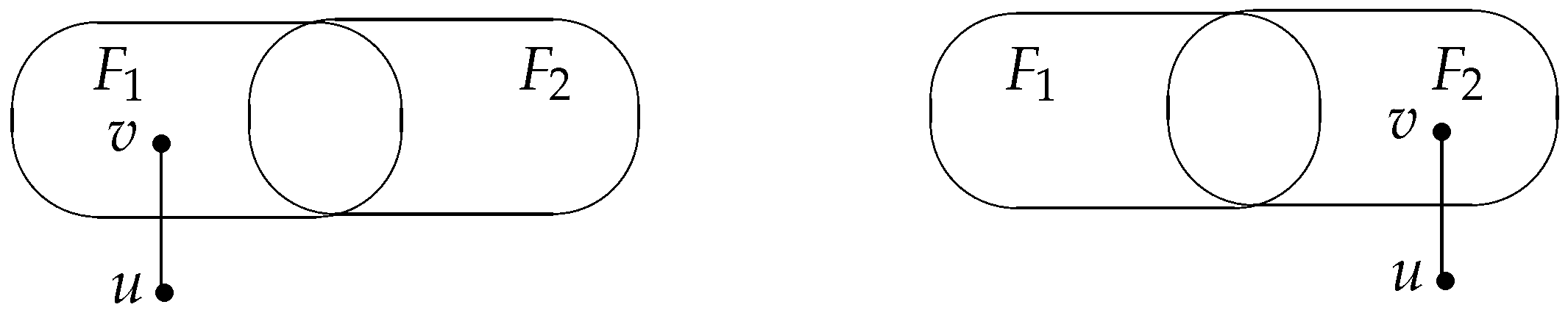
Before discussing the g-good-neighbor diagnosability of the arrangement graph $A_{n,k}$ under the MM${}^{*}$ model (Figure 3), we first give an existing result.

Theorem 7

([1,23]). A system $G=(V,E)$ is g-good-neighbor t-diagnosable under the $M{M}^{*}$ model if and only if for each distinct pair of g-good-neighbor faulty subsets $F_1$ and $F_2$ of V with $|F_1|\le t$ and $|F_2|\le t$ satisfies one of the following conditions. (1) There are two vertices $u,w\in V\backslash (F_1\cup F_2)$ and there is a vertex $v\in F_1∆F_2$ such that $uw\in E$ and $vw\in E$. (2) There are two vertices $u,v\in F_1\backslash F_2$ and there is a vertex $w\in V\backslash (F_1\cup F_2)$ such that $uw\in E$ and $vw\in E$. (3) There are two vertices $u,v\in F_2\backslash F_1$ and there is a vertex $w\in V\backslash (F_1\cup F_2)$ such that $uw\in E$ and $vw\in E$.

Lemma 22.

Let $n\ge 3$, $2\le k<n$ and $0\le g<n-k$. Then, the g-good-neighbor diagnosability of the arrangement graph $A_{n,k}$ under the MM* model is less than or equal to $[(g+1)(k-1)+1](n-k)$, i.e., $t_g(A_{n,k})\le [(g+1)(k-1)+1](n-k)$.

Proof. 

Let X be defined in Lemma 15, and let $F_1=N_{A_{n,k}}(X)$, $F_2=X\cup N_{A_{n,k}}(X)$. By Lemma 14, $|F_1|=[(g+1)(k-1)+1](n-k)-g$, $|F_2|=|X|+|F_1|=[(g+1)(k-1)+1](n-k)+1$, $\delta (A_{n,k}-F_1)\ge g$ and $\delta (A_{n,k}-F_2)\ge g$. Therefore, $F_1$ and $F_2$ are g-good-neighbor faulty sets of $A_{n,k}$ with $|F_1|=[(g+1)(k-1)+1](n-k)-g$ and $|F_2|=[(g+1)(k-1)+1](n-k)+1$.

We will prove that $A_{n,k}$ is not g-good-neighbor $([(g+1)(k-1)+1](n-k)+1)$-diagnosable. Since $X=F_1∆F_2$ and $N_{A_{n,k}}(X)=F_1\subset F_2$, there is no edge of $A_{n,k}$ between $V(A_{n,k})\backslash (F_1\cup F_2)$ and $F_1∆F_2$. By Theorem 7, we can show that $A_{n,k}$ is not g-good-neighbor $([(g+1)(k-1)+1](n-k)+1)$-diagnosable under the MM* model. Hence, by the definition of the g-good-neighbor diagnosability, we show that the g-good-neighbor diagnosability of $A_{n,k}$ is less than $[(g+1)(k-1)+1](n-k)+1$, i.e., $t_g(A_{n,k})\le [(g+1)(k-1)+1](n-k)$. □

Lemma 23.

Let $n,k,g$ be positive integers such that $n\ge 4$, $3\le k\le n-2,3\le g<n-k$. Then, the arrangement graph $A_{n,k}$ is g-good-neighbor $(((g+1)(k-2)+2-\lfloor \frac{{(g+1)}^2}{2}\rfloor )(n-k)+g+1)$-diagnosable under the MM* model.

Proof. 

By the definition of the g-good-neighbor diagnosability, it is sufficient to show that $A_{n,k}$ is g-good-neighbor $(((g+1)(k-2)+2-\lfloor \frac{{(g+1)}^2}{2}\rfloor )(n-k)+g+1)$-diagnosable for $3\le g\le n-k-1$.

By Theorem 7, suppose, on the contrary, that there are two distinct g-good-neighbor faulty subsets $F_1$ and $F_2$ of $A_{n,k}$ with $|F_1|\le ((g+1)(k-2)+2-\lfloor \frac{{(g+1)}^2}{2}\rfloor )(n-k)+g+1$ and $|F_2|\le ((g+1)(k-2)+2-\lfloor \frac{{(g+1)}^2}{2}\rfloor )(n-k)+g+1$, but the vertex set pair $(F_1,F_2)$ is not satisfied with any condition in Theorem 7. Without loss of generality, assume that $F_2\backslash F_1\ne \mathsf{\varnothing }.$ Similar to the discussion on $V(A_{n,k})=F_1\cup F_2$ in Lemma 16, we can show $V(A_{n,k})\ne F_1\cup F_2$.

Claim 1.$A_{n,k}-F_1-F_2$ has no isolated vertex.

Since $F_1$ is a g-good neighbor faulty set, for an arbitrary vertex $u\in V(A_{n,k})\backslash F_1$, $|N_{A_{n,k}-F_1}(u)|\ge g$. Suppose, on the contrary, that $A_{n,k}-F_1-F_2$ has at least one isolated vertex x. Since $F_1$ is a g-good neighbor faulty set and $g\ge 3$, there are at least two vertices $u,v\in F_2\backslash F_1$ such that $u,v$ are adjacent to x. According to the hypothesis, the vertex set pair $(F_1,F_2)$ is not satisfied with any condition in Theorem 7, by Condition (3) of Theorem 7, a contradiction. Therefore, there are at most one vertex $u\in F_2\backslash F_1$ such that u are adjacent to x. Thus, $|N_{A_{n,k}-F_1}(x)|=1$, a contradiction to that $F_1$ is a g-good neighbor faulty set, where $g\ge 3$. Thus, $A_{n,k}-F_1-F_2$ has no isolated vertex. The proof of Claim 1 is complete.

Let $u\in V(A_{n,k})\backslash (F_1\cup F_2)$. By Claim 1, $\delta (A_{n,k}-F_1-F_2)\ge 1$. Since the vertex set pair $(F_1,F_2)$ is not satisfied with any condition in Theorem 7, by the condition (1) of Theorem 7, for any pair of adjacent vertices $u,w\in V(A_{n,k})\backslash (F_1\cup F_2)$, there is no vertex $v\in F_1∆F_2$ such that $uw\in E(A_{n,k})$ and $uv\in E(A_{n,k})$. It follows that u has no neighbor in $F_1∆F_2$. Since u is taken arbitrarily, there is no edge between $V(A_{n,k})\backslash (F_1\cup F_2)$ and $F_1∆F_2$.

Since $F_2\backslash F_1\ne \mathsf{\varnothing }$ and $F_1$ is a g-good-neighbor faulty set, we have that ${\delta }_{A_{n,k}}([F_2\backslash F_1])\ge g$, $\delta (A_{n,k}-F_2-F_1)\ge g$ and $|F_2\backslash F_1|\ge g+1$. Since both $F_1$ and $F_2$ are g-good-neighbor faulty sets, and there is no edge between $V(A_{n,k})\backslash (F_1\cup F_2)$ and $F_1∆F_2$, $F_1\cap F_2$ is a g-good-neighbor cut of $A_{n,k}$. By Lemma 13, we have $|F_1\cap F_2|\ge ((g+1)(k-2)+2-\lfloor \frac{{(g+1)}^2}{2}\rfloor )(n-k)+1$. Therefore, $|F_2|=|F_2\backslash F_1|+|F_1\cap F_2|\ge g+1+((g+1)(k-2)+2-\lfloor \frac{{(g+1)}^2}{2}\rfloor )(n-k)+1=((g+1)(k-2)+2-\lfloor \frac{{(g+1)}^2}{2}\rfloor )(n-k)+g+2$, which contradicts $|F_2|\le ((g+1)(k-2)+2-\lfloor \frac{{(g+1)}^2}{2}\rfloor )(n-k)+g+1$. Therefore, $A_{n,k}$ is g-good-neighbor $(((g+1)(k-2)+2-\lfloor \frac{{(g+1)}^2}{2}\rfloor )(n-k)+g+1)$-diagnosable and $t_g(A_{n,k})\ge ((g+1)(k-2)+2-\lfloor \frac{{(g+1)}^2}{2}\rfloor )(n-k)+g+1$. The proof is complete. □

Combining Lemmas 22 and 23, we have the following theorem.

Theorem 8.

Let $n,k,g$ be positive integers such that $n\ge 4$, $3\le k\le n-2,3\le g<n-k$. Then, $((g+1)(k-2)+2-\lfloor \frac{{(g+1)}^2}{2}\rfloor )(n-k)+g+1\le t_g(A_{n,k})\le [(g+1)(k-1)+1](n-k)$ under the MM* model.

Theorem 9

([34]). Let $A_{n,k}$ be an n-dimensional arrangement graph and $3\le k<n$. Then, the diagnosability of $A_{n,k}$ is $k(n-k)$, i.e., $t(A_{n,k})=k(n-k)$ under the MM* model.

Lemma 24

([30]). $A_{n,k}$ is hamiltonian for $1\le k\le n-1$.

A component of a graph G is odd according as it has an odd number of vertices. We denote by $o(G)$ the number of odd component of G.

Theorem 10

([33]). A graph $G=(V,E)$ has a perfect matching if and only if $o(G-S)\le |S|$ for all $S\subseteq V$.

Lemma 25.

Let $n\ge 8$ and $2\le k<n$. Then, $t_1(A_{n,k})\ge (2k-1)(n-k)$ under the MM${}^{*}$ model.

Proof. 

By the definition of 1-good-neighbor diagnosability, it is sufficient to show that $A_{n,k}$ is 1-good-neighbor $(2k-1)(n-k)$-diagnosable.

By Theorem 7, suppose, on the contrary, that there are two distinct 1-good-neighbor faulty subsets $F_1$ and $F_2$ of $A_{n,k}$ with $|F_1|\le (2k-1)(n-k)$ and $|F_2|\le (2k-1)(n-k)$, but the vertex set pair $(F_1,F_2)$ is not satisfied with any condition in Theorem 7. Without loss of generality, suppose that $F_2\backslash F_1\ne \mathsf{\varnothing }.$ Assume $V(A_{n,k})=F_1\cup F_2$. We have that $\frac{n!}{(n-k)!}=|V(A_{n,k})|=|F_1\cup F_2|=|F_1|+|F_2|-|F_1\cap F_2|\le |F_1|+|F_2|\le 2(2k-1)(n-k)$. When $k=2$, $n^2-n=\frac{n!}{(n-2)!}=|V(A_{n,2})|=|F_1\cup F_2|\le 6n-12$, a contradiction to $n\ge 5$. Therefore, $V(A_{n,2})\ne F_1\cup F_2$. When $k=3$, $\frac{n!}{(n-k)!}=n^3-3n^2+2n$. Note $n^3-3n^2+2n\le \frac{n!}{(n-k)!}$ for $k\ge 3$. Thus, $2(2k-1)(n-k)\le 2(2(n-1)-1)(n-3)\le 4n^2-18n+18$. In fact, $n^3-3n^2+2n>4n^2-18n+18$ when $n\ge 5$. This is a contradiction. Therefore, $V(A_{n,k})\ne F_1\cup F_2$.

Claim 1.$A_{n,k}-F_1-F_2$ has no isolated vertex.

Suppose, on the contrary, that $A_{n,k}-F_1-F_2$ has at least one isolated vertex w. Since $F_1$ is a 1-good-neighbor faulty set, there is a vertex $u\in F_2\backslash F_1$ such that u is adjacent to w. Since the vertex set pair $(F_1,F_2)$ is not satisfied with any condition in Theorem 7, there is at most one vertex $u\in F_2\backslash F_1$ such that u is adjacent to w. Thus, there is just a vertex $u\in F_2\backslash F_1$ such that u is adjacent to w. Similarly, we can show that there is just a vertex $v\in F_1\backslash F_2$ such that v is adjacent to w when $F_1\backslash F_2\ne \mathsf{\varnothing }$. Suppose $F_1\backslash F_2=\mathsf{\varnothing }$. Then, $F_1\subseteq F_2$. Since $F_2$ is a 1-good neighbor faulty set, $A_{n,k}-F_2=A_{n,k}-F_1-F_2$ has no isolated vertex. Therefore, $F_1\backslash F_2\ne \mathsf{\varnothing }$ as follows. Let $W\subseteq V(A_{n,k})\backslash (F_1\cup F_2)$ be the set of isolated vertices in $A_{n,k}[V(A_{n,k})\backslash (F_1\cup F_2)]$, and let H be the subgraph induced by the vertex set $V(A_{n,k})\backslash (F_1\cup F_2\cup W)$. Then, for any $w\in W$, there are $(k(n-k)-2)$ neighbors in $F_1\cap F_2$. Since $|V(A_{n,k})|$ is even and Lemma 24, $A_{n,k}$ has a perfect matching. By Theorem 10, $|W|\le o(G-(F_1\cup F_2))\le |F_1\cup F_2|\le |F_1|+|F_2|-|F_1\cap F_2|\le 2(2k-1)(n-k)-(k(n-k)-2)=(n-k)(3k-2)+2\le 3n^2-11n+12$. In particular, $|W|\le 4n-6$ when $k=2$. When $k=2$, $n^2-n=|V(A_{n,2})|=|F_1\cup F_2|+|W|\le 2(4n-6)=8n-12$. This is a contradiction to $n\ge 8$. Thus, $V(H)\ne \mathsf{\varnothing }$. When $k=3$, $\frac{n!}{(n-k)!}=n^3-3n^2+2n$. Note $n^3-3n^2+2n\le \frac{n!}{(n-k)!}$ for $k\ge 3$. Note that $n^3-3n^2+2n=|V(A_{n,k})|=|F_1\cup F_2|+|W|\le 2(3n^2-11n+12)=6n^2-22n+24$. This is a contradiction to $n\ge 8$. Thus, $V(H)\ne \mathsf{\varnothing }$. Since the vertex set pair $(F_1,F_2)$ is not satisfied with the condition (1) of Theorem 7, and any vertex of $V(H)$ is not isolated in H, we show that there is no edge between $V(H)$ and $F_1∆F_2$. Thus, $F_1\cap F_2$ is a vertex cut of $A_{n,k}$ and $\delta (A_{n,k}-(F_1\cap F_2))\ge 1$, i.e., $F_1\cap F_2$ is a 1-good-neighbor cut of $A_{n,k}$. By Lemma 10, $|F_1\cap F_2|\ge (2k-1)(n-k)-1$. Because $|F_1|\le (2k-1)(n-k)$, $|F_2|\le (2k-1)(n-k)$, and neither $F_1\backslash F_2$ nor $F_2\backslash F_1$ is empty, we have $|F_1\backslash F_2|=|F_2\backslash F_1|=1$. Let $F_1\backslash F_2=\left\{v_1\right\}$ and $F_2\backslash F_1=\left\{v_2\right\}$. Then, for any vertex $w\in W$, w are adjacent to $v_1$ and $v_2$. Suppose that $v_1$ is adjacent to $v_2$. Then, $v_1{v}_{2}v{v}_1$ is a three-cycle and $|N(\{v_1,v_{2,}v\})|=3[(k-1)(n-k)-1]+n-k+1>(2k-1)(n-k)-1\ge |F_1\cap F_2|$, a contradiction. Therefore, suppose that $v_1$ is not adjacent to $v_2$. According to Lemma 9, there are at most two common neighbors for any pair of vertices in $A_{n,k}$, it follows that there are at most three isolated vertices in $A_{n,k}-F_1-F_2$, i.e., $|W|\le 2$.

Suppose that there is exactly one isolated vertex v in $A_{n,k}-F_1-F_2$. Let $v_1$ and $v_2$ be adjacent to v. Then, $N_{A_{n,k}}(v)\backslash \{v_1,v_2\}\subseteq F_1\cap F_2$ and $|N_{A_{n,k}}(v)\cap (F_1\cap F_2)|=k(n-k)-2$. Note that $|N_{A_{n,k}}(v_1)\cap (F_1\cap F_2)|=k(n-k)-1$ and $|N_{A_{n,k}}(v_2)\cap (F_1\cap F_2)|=k(n-k)-1$. By Lemma 9, $|F_1\cap F_2|\ge k(n-k)-2+k(n-k)-1+k(n-k)-1-2(n-k-1)-2=(3k-2)(n-k)-4.$ It follows that $|F_2|=|F_2\backslash F_1|+|F_1\cap F_2|\ge 1+(3k-2)(n-k)-4=(3k-2)(n-k)-3>(2k-1)(n-k)(n\ge 8)$, which contradicts $|F_2|\le (2k-1)(n-k)$.

Suppose that there are exactly two isolated vertices v and w in $A_{n,k}-F_1-F_2$. Let $v_1$ and $v_2$ be adjacent to v and w, respectively. Since $v_1,v_2\in N_{A_{n,k}}(\{v,w\})$, by Lemma 9, $|N_{A_{n,k}}(\{v,w\})\cap (F_1\cap F_2)|=2(k(n-k)-2)$. Note that $|F_1\cap F_2|\le (2k-1)(n-k)-1$. If $n>k+3$, then $2(k(n-k)-2)>(2k-1)(n-k)-1$, a contradiction. Thus, $n\le k+3$. Since $n\ge k+1$, $k+1\le n\le k+3$. If $n=k+1$, then, by Lemma 9, a contradiction to $|W|=2$. Suppose that $n=k+2$. Then, $A_{n,k}=A_{n,n-2}$. By the proof of Lemma 3.2 ([18]), $A_{n,n-2}-F_1-F_2$ has no isolated vertex. Suppose that $n=k+3$. Then, $2(k(n-k)-2)=(2k-1)(n-k)-1=6n-22$. By Lemma 1, let $v_1=(1,2,\dots ,n-4,n-3)$.Without loss of generality, suppose $v=(1,2,\dots ,n-4,n)$ and $w=(n,2,\dots ,n-4,n-3)$. Then, the vertex $v^{\prime }=(1,n-1,\dots ,n-4,n-3)$ is not adjacent to v and w. Thus, $|F_1\cap F_2|>(2k-1)(n-k)-1$, a contradiction. The proof of Claim 1 is complete.

Let $u\in V(A_{n,k})\backslash (F_1\cup F_2)$. By Claim 1, u has at least one neighbor in $A_{n,k}-F_1-F_2$. Since the vertex set pair $(F_1,F_2)$ is not satisfied with any condition in Theorem 7, by the condition (1) of Theorem 7, for any pair of adjacent vertices $u,w\in V(A_{n,k})\backslash (F_1\cup F_2)$, there is no vertex $v\in F_1∆F_2$ such that $uw\in E(A_{n,k})$ and $vw\in E(A_{n,k})$. It follows that u has no neighbor in $F_1∆F_2$. Since u is taken arbitrarily, there is no edge between $V(A_{n,k})\backslash (F_1\cup F_2)$ and $F_1∆F_2$. Since $F_2\backslash F_1\ne \mathsf{\varnothing }$ and $F_1$ is a 1-good-neighbor faulty set, ${\delta }_{A_{n,k}}([F_2\backslash F_1])\ge 1$ and $|F_2\backslash F_1|\ge 2$. Since both $F_1$ and $F_2$ are 1-good-neighbor faulty sets, and there is no edge between $V(A_{n,k})\backslash (F_1\cup F_2)$ and $F_1∆F_2$, $F_1\cap F_2$ is a 1-good-neighbor cut of $A_{n,k}$. By Lemma 10, we have $|F_1\cap F_2|\ge (2k-1)(n-k)-1$. Therefore, $|F_2|=|F_2\backslash F_1|+|F_1\cap F_2|\ge 2+((2k-1)(n-k)-1)=(2k-1)(n-k)+1$, which contradicts $|F_2|\le (3k-2)(n-k)$. Therefore, $A_{n,k}$ is 1-good-neighbor $(3k-2)(n-k)$-diagnosable and $t_1(A_{n,k})\ge (3k-2)(n-k)$. The proof is complete. □

Combining Lemmas 22 and 25, we have the following theorem.

Theorem 11.

Let $n\ge 8$. Then, $t_1(A_{n,k})=(2k-1)(n-k)$ under the MM${}^{*}$ model.

Lemma 26.

Let $n\ge 8$ and $k\in \{i:i=3,\dots ,n-5\}\cup \{n-2,n-1\}$. Then, $t_2(A_{n,k})\ge (3k-2)(n-k)$ under the MM${}^{*}$ model.

Proof. 

By the definition of the 2-good-neighbor diagnosability, it is sufficient to show that $A_{n,k}$ is g-good-neighbor $(3k-2)(n-k)$-diagnosable.

By Theorem 7, suppose, on the contrary, that there are two distinct g-good-neighbor faulty subsets $F_1$ and $F_2$ of $A_{n,k}$ with $|F_1|\le (3k-2)(n-k)$ and $|F_2|\le (3k-2)(n-k)$, but the vertex set pair $(F_1,F_2)$ is not satisfied with any condition in Theorem 7. Without loss of generality, suppose that $F_2\backslash F_1\ne \mathsf{\varnothing }.$ Similar to the discussion on $V(A_{n,k})=F_1\cup F_2$ in Lemma 18, we have $V(A_{n,k})\ne F_1\cup F_2$.

Claim 1.$A_{n,k}-F_1-F_2$ has no isolated vertex.

Since $F_1$ is a 2-good neighbor faulty set, for an arbitrary vertex $u\in V(A_{n,k})\backslash F_1$, $|N_{A_{n,k}-F_1}(u)|\ge 2$. Suppose, on the contrary, that $A_{n,k}-F_1-F_2$ has at least one isolated vertex x. Since $F_1$ is a 2-good neighbor faulty set, there are at least two vertices $u,v\in F_2\backslash F_1$ such that $u,v$ are adjacent to x. According to the hypothesis, the vertex set pair $(F_1,F_2)$ is not satisfied with any condition in Theorem 7, by the condition (3) of Theorem 7, a contradiction. Therefore, there are at most one vertex $u\in F_2\backslash F_1$ such that u are adjacent to x. Thus, $|N_{A_{n,k}-F_1}(x)|=1$, a contradiction to that $F_1$ is a 2-good neighbor faulty set. Thus, $A_{n,k}-F_1-F_2$ has no isolated vertex. The proof of Claim 1 is complete.

Let $u\in V(A_{n,k})\backslash (F_1\cup F_2)$. By Claim 1, $\delta (A_{n,k}-F_1-F_2)\ge 1$. Since the vertex set pair $(F_1,F_2)$ is not satisfied with any condition in Theorem 7, by the condition (1) of Theorem 7, for any pair of adjacent vertices $u,w\in V(A_{n,k})\backslash (F_1\cup F_2)$, there is no vertex $v\in F_1∆F_2$ such that $uw\in E(A_{n,k})$ and $uv\in E(A_{n,k})$. It follows that u has no neighbor in $F_1∆F_2$. Since u is taken arbitrarily, there is no edge between $V(A_{n,k})\backslash (F_1\cup F_2)$ and $F_1∆F_2$.

Since $F_2\backslash F_1\ne \mathsf{\varnothing }$ and $F_1$ is a 2-good-neighbor faulty set, we have that ${\delta }_{A_{n,k}}([F_2\backslash F_1])\ge 2$, $\delta (A_{n,k}-F_2-F_1)\ge 2$ and $|F_2\backslash F_1|\ge 2+1=3$. Since both $F_1$ and $F_2$ are 2-good-neighbor faulty sets, and there is no edge between $V(A_{n,k})\backslash (F_1\cup F_2)$ and $F_1∆F_2$, $F_1\cap F_2$ is a 2-good-neighbor cut of $A_{n,k}$. By Lemma 11, we have $|F_1\cap F_2|\ge (3k-2)(n-k)-2$. Therefore, $|F_2|=|F_2\backslash F_1|+|F_1\cap F_2|\ge 3+(3k-2)(n-k)-2=(3k-2)(n-k)+1$, which contradicts $|F_2|\le (3k-2)(n-k)$. Therefore, $A_{n,k}$ is 2-good-neighbor $(3k-2)(n-k)$-diagnosable and $t_2(A_{n,k})\ge (3k-2)(n-k)$. The proof is complete. □

Combining Lemmas 22 and 26, we have the following theorem.

Theorem 12.

Let $n\ge 8$ and $k\in \{i:i=3,\dots ,n-5\}\cup \{n-2,n-1\}$. Then, $t_2(A_{n,k})=(3k-2)(n-k)$ under the MM${}^{*}$ model.

Lemma 27.

For $n\ge 8$, $t_2(A_{n,2})\le 4n-9$ under the MM${}^{*}$ model.

Proof. 

Let X be defined in Lemma 19, and let $F_1=N_{A_{n,2}}(X)$, $F_2=X\cup N_{A_{n,2}}(X)$. By Lemma 19, $|F_1|=4n-12$, $|F_2|=|X|+|F_1|=4n-8$, $\delta (A_{n,2}-F_1)\ge 2$ and $\delta (A_{n,2}-F_2)\ge 2$. Therefore, $F_1$ and $F_2$ are 2-good-neighbor faulty sets of $A_{n,2}$ with $|F_1|=4n-12$ and $|F_2|=4n-8$.

We will prove $A_{n,2}$ is not 2-good-neighbor $(4n-8)$-diagnosable. Since $X=F_1∆F_2$ and $N_{A_{n,k}}(X)=F_1\subset F_2$, there is no edge of $A_{n,2}$ between $V(A_{n,2})\backslash (F_1\cup F_2)$ and $F_1∆F_2$. By Theorem 7, we show that $A_{n,2}$ is not 2-good-neighbor $(4n-8)$-diagnosable under the MM${}^{*}$ model. Hence, by the definition of the 2-good-neighbor diagnosability, we show that the 2-good-neighbor diagnosability of $A_{n,2}$ is less than $4n-8$, i.e., $t_g(A_{n,2})\le 4n-9$. □

Lemma 28.

For $n\ge 8$, $t_2(A_{n,2})\ge 4n-9$ under the MM${}^{*}$ model.

Proof. 

By the definition of the 2-good-neighbor diagnosability, it is sufficient to show that $A_{n,k}$ is 2-good-neighbor $(4n-9)$-diagnosable.

By Theorem 7, suppose, on the contrary, that there are two distinct 2-good-neighbor faulty subsets $F_1$ and $F_2$ of $A_{n,k}$ with $|F_1|\le 4n-9$ and $|F_2|\le 4n-9$, but the vertex set pair $(F_1,F_2)$ is not satisfied with any condition in Theorem 7. Without loss of generality, suppose that $F_2\backslash F_1\ne \mathsf{\varnothing }.$ Similar to the discussion on $V(A_{n,k})=F_1\cup F_2$ in Lemma 21, we have $V(A_{n,k})\ne F_1\cup F_2$.

Claim 1.$A_{n,k}-F_1-F_2$ has no isolated vertex.

Since $F_1$ is a 2-good neighbor faulty set, for an arbitrary vertex $u\in V(A_{n,k})\backslash F_1$, $|N_{A_{n,k}-F_1}(u)|\ge 2$. Suppose, on the contrary, that $A_{n,k}-F_1-F_2$ has at least one isolated vertex x. Since $F_1$ is a 2-good neighbor faulty set, there are at least two vertices $u,v\in F_2\backslash F_1$ such that $u,v$ are adjacent to x. According to the hypothesis, the vertex set pair $(F_1,F_2)$ is not satisfied with any condition in Theorem 7, by the condition (3) of Theorem 7, a contradiction. Therefore, there are at most one vertex $u\in F_2\backslash F_1$ such that u are adjacent to x. Thus, $|N_{A_{n,k}-F_1}(x)|=1$, a contradiction to that $F_1$ is a 2-good neighbor faulty set. Thus, $A_{n,k}-F_1-F_2$ has no isolated vertex. The proof of Claim 1 is complete.

Let $u\in V(A_{n,k})\backslash (F_1\cup F_2)$. By Claim 1, $\delta (A_{n,k}-F_1-F_2)\ge 1$. Since the vertex set pair $(F_1,F_2)$ is not satisfied with any condition in Theorem 7, by the condition (1) of Theorem 7, for any pair of adjacent vertices $u,w\in V(A_{n,k})\backslash (F_1\cup F_2)$, there is no vertex $v\in F_1∆F_2$ such that $uw\in E(A_{n,k})$ and $uv\in E(A_{n,k})$. It follows that u has no neighbor in $F_1∆F_2$. Since u is taken arbitrarily, there is no edge between $V(A_{n,k})\backslash (F_1\cup F_2)$ and $F_1∆F_2$.

Since $F_2\backslash F_1\ne \mathsf{\varnothing }$ and $F_1$ is a 2-good-neighbor faulty set, we have that ${\delta }_{A_{n,k}}([F_2\backslash F_1])\ge 2$, $\delta (A_{n,k}-F_2-F_1)\ge 2$ and $|F_2\backslash F_1|\ge 2+1=3$. Since both $F_1$ and $F_2$ are 2-good-neighbor faulty sets, and there is no edge between $V(A_{n,k})\backslash (F_1\cup F_2)$ and $F_1∆F_2$, $F_1\cap F_2$ is a 2-good-neighbor cut of $A_{n,k}$. By Lemma 11, we have $|F_1\cap F_2|\ge 4n-12$. If $|F_1\cap F_2|=4n-12$, then, by Lemma 12, $|F_2\backslash F_1|=4$. If $|F_1\cap F_2|=4n-11$ or $4n-10$, then $|F_2\backslash F_1|\le 2$, a contradiction to that $\delta (A_{n,2}[F_1\backslash F_2])\ge 2$. Therefore, $|F_2|=|F_2\backslash F_1|+|F_1\cap F_2|\ge 4+(4n-12)=4n-8$, which contradicts with that $|F_2|\le 4n-9$. Therefore, $A_{n,k}$ is 2-good-neighbor $(4n-9)$-diagnosable and $t_2(A_{n,k})\ge 4n-9$. The proof is complete. □

Combining Lemmas 27 and 28, we have the following theorem.

Theorem 13.

Let $n\ge 8$. Then, $t_2(A_{n,2})=4n-9$ under the MM${}^{*}$ model.

5. Conclusions

The conditional diagnosability of a multiprocessor system is an important research topic for fault tolerance of the system. In this paper, we investigate the problem of g-good-neighbor diagnosability of the $(n,k)$-arrangement graph $A_{n,k}$, and present the g-good-neighbor diagnosability of $A_{n,k}$ under the PMC model and MM* model. The work will help engineers to develop more different networks.

References

- Dahbura, A.T.; Masson, G.M. An O(n2.5) Fault identification algorithm for diagnosable systems. IEEE Trans. Comput. 1984, 33, 486–492. [Google Scholar] [CrossRef]
- Fan, J. Diagnosability of crossed cubes under the comparison diagnosis model. IEEE Trans. Parallel Distrib. Syst. 2002, 13, 1099–1104. [Google Scholar]
- Lai, P.L.; Tan, J.J.M.; Chang, C.-P.; Hsu, L.-H. Conditional diagnosability measures for large multiprocessor systems. IEEE Trans. Comput. 2005, 54, 165–175. [Google Scholar] [Green Version]
- Preparata, F.P.; Metze, G.; Chien, R.T. On the connection assignment problem of diagnosable systems. IEEE Trans. Comput. EC 1967, 16, 848–854. [Google Scholar] [CrossRef]
- Maeng, J.; Malek, M. A comparison connection assignment for self-diagnosis of multiprocessor systems. In Proceedings of the 11th International Symposium on Fault-Tolerant Computing, Portland, ME, USA, 24–26 June 1981; pp. 173–175. [Google Scholar]
- Peng, S.-L.; Lin, C.-K.; Tan, J.J.M.; Hsu, L.-H. The g-good-neighbor conditional diagnosability of hypercube under PMC model. Appl. Math. Comput. 2012, 218, 10406–10412. [Google Scholar] [CrossRef]
- Wang, S.; Han, W. The g-good-neighbor conditional diagnosability of n-dimensional hypercubes under the MM* model. Inf. Process. Lett. 2016, 116, 574–577. [Google Scholar] [CrossRef]
- Jirimutu, J.; Wang, S. The 1-good-neighbor diagnosability of alternating group graph networks under the PMC model and MM* model. Recent Patents Comput. Sci. 2017, 10, 108–115. [Google Scholar] [CrossRef]
- Ren, Y.; Wang, S. The g-good-neighbor diagnosability of locally twisted cubes. Theor. Comput. Sci. 2017, 697, 91–97. [Google Scholar] [CrossRef]
- Ren, Y.; Wang, S. Some properties of the g-good-neighbor (g-extra) diagnosability of a multiprocessor system. Am. J. Comput. Math. 2016, 6, 259–266. [Google Scholar] [CrossRef]
- Wang, M.; Guo, Y.; Wang, S. The 1-good-neighbor diagnosability of Cayley graphs generated by transposition trees under the PMC model and MM* model. Int. J. Comput. Math. 2017, 94, 620–631. [Google Scholar] [CrossRef]
- Wang, M.; Lin, Y.; Wang, S. The 2-good-neighbor diagnosability of Cayley graphs generated by transposition trees under the PMC model and MM* model. Theor. Comput. Sci. 2016, 628, 92–100. [Google Scholar] [CrossRef]
- Wang, M.; Lin, Y.; Wang, S. The 1-good-neighbor connectivity and diagnosability of Cayley graphs generated by complete graphs. Discr. Appl. Math. 2018, 246, 108–118. [Google Scholar] [CrossRef]
- Wang, M.; Lin, Y.; Wang, S. The connectivity and nature diagnosability of expanded k-ary n-cubes. RAIRO-Theor. Inf. Appl. 2017, 51, 71–89. [Google Scholar] [CrossRef]
- Wang, M.; Lin, Y.; Wang, S. The nature diagnosability of bubble-sort star graph networks under the PMC model and MM* model. Int. J. Eng. Appl. Sci. 2017, 4, 55–60. [Google Scholar]
- Wang, S.; Yang, Y. The 2-good-neighbor (2-extra) diagnosability of alternating group graph networks under the PMC model and MM* model. Appl. Math. Comput. 2017, 305, 241–250. [Google Scholar] [CrossRef]
- Wang, S.; Wang, Z.; Wang, M. The 2-good-neighbor connectivity and 2-good-neighbor diagnosability of bubble-sort star graph networks. Discr. Appl. Math. 2017, 217, 691–706. [Google Scholar] [CrossRef]
- Wang, S.; Zhao, L. A note on the nature diagnosability of alternating group graphs under the PMC model and MM* model. J. Interconnect. Netw. 2018, 18, 1850005. [Google Scholar] [CrossRef]
- Wang, S.; Wang, Z.; Wang, M.; Han, W. The g-good-neighbor conditional diagnosability of star graph networks under the PMC model and MM* model. Front. Math. China 2017, 12, 1221–1234. [Google Scholar] [CrossRef]
- Wang, S.; Ma, X.; Ren, Y. The tightly super 2-good-neighbor connectivity and 2-good-neighbor diagnosability of crossed cubes. Int. J. New Technol. Res. 2017, 3, 70–82. [Google Scholar]
- Wang, Y.; Wang, S.; Wang, Z. The 1-good-neighbor diagnosability of shuffle-cubes. Int. J. New Technol. Res. 2017, 3, 66–73. [Google Scholar]
- Xu, X.; Zhou, S.; Li, J. Reliability of complete cubic networks under the condition of g-good-neighbor. Comput. J. 2017, 60, 625–637. [Google Scholar] [CrossRef]
- Yuan, J.; Liu, A.; Ma, X.; Liu, X.; Qin, X.; Zhang, J. The g-good-neighbor conditional diagnosability of k-ary n-cubes under the PMC model and MM* model. IEEE Trans. Parallel Distrib. Syst. 2015, 26, 1165–1177. [Google Scholar] [CrossRef]
- Yuan, J.; Liu, A.; Qin, X.; Zhang, J.; Li, J. g-Good-neighbor conditional diagnosability measures for 3-ary n-cube networks. Theor. Comput. Sci. 2016, 622, 144–162. [Google Scholar] [CrossRef]
- Akers, S.B.; Krishnamurthy, B. Akers, Balakrishnan Krishnamurthy, A group theoretic model for symmetric interconnection networks. IEEE Trans. Comput. 1989, 38, 555–566. [Google Scholar]
- Day, K.; Tripathi, A. Arrangement graphs: A class of generalized star graphs. Inf. Process. Lett. 1992, 42, 235–241. [Google Scholar] [CrossRef]
- Cheng, E.; Lipták, L.; Yuan, A. Linearly many faults in arrangement graphs. Networks 2013, 61, 281–289. [Google Scholar] [CrossRef]
- Cheng, E.; Qiu, K.; Shen, Z. On the restricted connectivity of the arrangement graph. J. Supercomput. 2017, 73, 3669–3682. [Google Scholar] [CrossRef]
- Chiang, W.-K.; Chen, R.-J. On the arrangement graph. Inf. Process. Lett. 1998, 66, 215–219. [Google Scholar] [CrossRef]
- Day, K.; Tripathi, A. Embedding of cycles in arrangement graphs. IEEE Trans. Comput. 1993, 42, 1002–1006. [Google Scholar] [CrossRef]
- Lin, L.; Zhou, S.; Xu, L.; Wang, D. Conditional diagnosability of arrangement graphs under the PMC model. Theor. Comput. Sci. 2014, 548, 79–97. [Google Scholar] [CrossRef]
- Zhou, S.; Xu, J.M. Conditional fault tolerance of arrangement graphs. Inf. Process. Lett. 2011, 111, 1037–1043. [Google Scholar] [CrossRef]
- Bondy, J.A.; Murty, U.S.R. Graph Theory; Springer: New York, NY, USA, 2007. [Google Scholar]
- Wang, S.; Ma, X. Diagnosability of arrangement graphs with missing edges under MM* model. Appl. Math. Comput. to appear.
Figure 1.
The arrangement graph .
Figure 2.
Illustration of a distinguishable pair under the PMC model.
Figure 3.
Illustration of a distinguishable pair under the MM* model.
© 2018 by the authors. Licensee MDPI, Basel, Switzerland. This article is an open access article distributed under the terms and conditions of the Creative Commons Attribution (CC BY) license (http://creativecommons.org/licenses/by/4.0/).
Share and Cite
MDPI and ACS Style
Wang, S.; Ren, Y. g-Good-Neighbor Diagnosability of Arrangement Graphs under the PMC Model and MM* Model. Information 2018, 9, 275. https://doi.org/10.3390/info9110275
AMA Style
Wang S, Ren Y. g-Good-Neighbor Diagnosability of Arrangement Graphs under the PMC Model and MM* Model. Information. 2018; 9(11):275. https://doi.org/10.3390/info9110275
Chicago/Turabian StyleWang, Shiying, and Yunxia Ren. 2018. "g-Good-Neighbor Diagnosability of Arrangement Graphs under the PMC Model and MM* Model" Information 9, no. 11: 275. https://doi.org/10.3390/info9110275
Note that from the first issue of 2016, this journal uses article numbers instead of page numbers. See further details here.