A Diabetes Management Information System with Glucose Prediction

1
Scientific Initiation Program, Faculty ImesMercosur (IMESMERCOSUR), Governador Valadares 35010-161, Brazil
2
Postgraduate Program in Computational Modeling, Federal University of Juiz de Fora (UFJF), Juiz de Fora 36036-900, Brazil
*
Author to whom correspondence should be addressed.
Information 2018, 9(12), 319; https://doi.org/10.3390/info9120319
Submission received: 31 October 2018
/
Revised: 6 December 2018
/
Accepted: 7 December 2018
/
Published: 12 December 2018
(This article belongs to the Special Issue Information Technology: New Generations (ITNG 2018))
Abstract
:Diabetes has become a serious health concern. The use and popularization of blood glucose measurement devices have led to a tremendous increase on health for diabetics. Tracking and maintaining traceability between glucose measurements, insulin doses and carbohydrate intake can provide useful information to physicians, health professionals, and patients. This paper presents an information system, called GLUMIS (GLUcose Management Information System), aimed to support diabetes management activities. It is made of two modules, one for glucose prediction and one for data visualization and a reasoner to aid users in their treatment. Through integration with glucose measurement devices, it is possible to collect historical data on the treatment. In addition, the integration with a tool called the REALI System allows GLUMIS to also process data on insulin doses and eating habits. Quantitative and qualitative data were collected through an experimental case study involving 10 participants. It was able to demonstrate that the GLUMIS system is feasible. It was able to discover rules for predicting future values of blood glucose by processing the past history of measurements. Then, it presented reports that can help diabetics choose the amount of insulin they should take and the amount of carbohydrate they should consume during the day. Rules found by using one patient’s measurements were analyzed by a specialist that found three of them to be useful for improving the patient’s treatment. One such rule was “if glucose before breakfast then glucose at afternoon break in ”. The results obtained through the experimental study and other verifications associated with the algorithm created had a double objective. It was possible to show that participants, through a questionnaire, viewed the visualizations as easy, or very easy, to understand. The secondary objective showed that the innovative algorithm applied in the GLUMIS system allows the decision maker to have much more precision and less loss of information than in algorithms that require the data to be discretized.
1. Introduction
The disease characterized by making the patient constantly exhibit elevated levels of blood glucose is referred to as diabetes mellitus. There are three different diabetes mellitus types [1]. Type I diabetes mellitus refers to the stage of juvenile deviance when the pancreas does not produce enough insulin, or even produces no insulin at all. Type II diabetes mellitus is associated with the inability of the patient’s body to use the secreted insulin. There is also gestational diabetes that indicates the condition in which a woman, without diabetes, has high blood glucose levels during pregnancy.
Millions of people worldwide are afflicted by Diabetes. It is considered an epidemic disease in the United States and a growing disease in the world. It is predicted to continue to be a major health crisis even with the recent advances in treatment [2].
Diabetes treatment is done by controlling the values of blood glucose using artificial insulin and controlling quantity of carbohydrate intake. Controlling the values of glycated hemoglobin can lead to a healthy life for a diabetic [3]. Not following a diet, limiting sugar and carbohydrates, and not taking the necessary dosage of insulin can lead to serious health problems such as retinopathy, kidney damage, heart diseases and stroke [4].
Projections of the annual cost for diabetes treatment are updated every few years and each new prediction is higher than the previous one. A study from 2010 estimated that by 2030 the annual cost in the U.S. would be of $490 billion dollars [5], while a newer study from 2017 shows a prediction of $622 billion dollars [2]. In relation to the number of diabetics, it is estimated that there were 372 million diabetics in 2012 and this should increase to 552 million diabetics by 2030 [6,7]. New research already indicates the estimates up until 2040 [8].
Glucose measurement and control is aided by glucose monitoring devices, a more in-depth study about the history and future of glucose measurement devices can be seen on [9]. The most common type of glucose measurement device are the Blood Glucose Meters (BGMs) [10] which requires the user to perform a fingerstick test to acquire blood for the test. There is also the use of non-invasive glucose monitoring (NGM) [11], which have the benefit of making a glucose test more convenient by not needing a fingerstick test, but, on the other side, it doesn’t give a precision as good as a traditional BGM and are not recommended to be used as the only device to take medications and make treatment decisions [12].
Continuous Glucose Monitoring Systems (CGMS) provides a large number of glucose measurements by measuring blood glucose at every few minutes. This makes them useful for detecting hypo-glycemia and hyper-glycemia and for choosing the insulin dosage [13,14]. This higher quantity of information available enables them to make a more complete glucose profile of the patient than blood glucose meters which only makes few measurements each day. However, their use in clinical practice is hampered by their accuracy, and this has led to research for better signal processing methods [15]. In addition, there are some details that should be noted [16,17]:
- Cost: this is the main limitation, as it is beyond the reach of most diabetics.
- May be invasive: most of the commercially-available CGMS are based on invasive techniques.
- Learning curve: It employs a complex procedure where the diabetic needs to be trained and educated to use it.
- Calibration: In some cases, the application of some calibration may be necessary to adjust the performance according to the established standards of glucose monitoring. In these cases, then, continuous devices do not completely eliminate the need for blood tests by a BGM.
A significant amount of data must be collected, processed and stored over time, for proper monitoring. The process of discovering knowledge through these data may consider visualization mechanisms to support the recognition of relevant information and its presentation to patients and physicians. Therefore, the information visualization can be referenced as part of a understanding process that aims to achieve in-depth knowledge about a topic and it is critical to create a consistent mental model associated with a particular situation [18], for example, the patient’s current condition and its evolution over time.
The composition of different points of view may allow the data analysis from different perspectives, complementing the information. Thus, a system that uses two or more distinct views to support the investigation of a subject is called Multiple Views. Such systems minimize the occurrence of misinterpretations when compared to analysis performed through a single view [19].
In view of this, there is a need for Systems capable of providing health care professionals and patients with useful information about in glucose concentration and its fluctuations throughout the day [20,21,22]. Moreover, tracking and maintaining traceability between glucose measurements, insulin doses and carbohydrate intake can provide useful information to physicians, health professionals, and patients. This may enable the prevention of hypoglycemia and allow the diabetic to maintain healthy levels of blood glucose concentration with a predicted glycemic variability.
Therefore, this paper presents an information system, called GLUMIS, aimed to support diabetes management activities. It encompasses a prediction rule-based method for glucose measurement, a reasoner and visualization elements. Through integration with BGM and NGM devices and CGMS, it is possible to collect historical treatment data and, with a REALI system, insulin doses and dietary habits can be processed. This paper is an extended version of a previously published paper on ITNG 2018 [23], and the differences between the original version and this extended one are explained on Section 2.
The data used in the experiment were obtained as a result of a partnership established with a medical clinic and has been protected for confidentiality reasons. Considering this real context, in order to obtain evidence on the system viability, an experimental study was carried out.
This article is structured by this introduction and Section 2 shows the background in which the proposal is inserted and some related work. Section 3 details the new classification algorithm proposed on this paper, which was named the Multidimensional Multiscale Forest (MMF). Section 4 presents the components of the GLUMIS system. In Section 5, the experiment was carried out and Section 6 provides the final considerations.
2. Background
Devices such as BGMs and CGMs do not allow the recording of additional information, such as insulin dosage and food intake, although they are useful for providing information on the current level of glucose. Such information, when put together, could be used to generate findings on current treatment, as well as unfolding and clues to future glycemic values.
Thus, an opportunity opens up for an integration between a system that records information on physical activity, food intake, and insulin doses, with another system that maintains glucose measurement records, with increased analytical capacity presenting more elaborate views. In addition, this system could use this combinatorial data explosion to find rules, model a patient’s profile, and then gain relevant knowledge for patients and physicians.
Prediction is usually modelled as a problem of classification, where there is a finite number of target classes. Moreover, the data outputted by CGMSs and BGMs is on a continuous domain, which leads the data to be discredited for it to work on traditional classification methods. A problem with making data discrete is the loss of information, which might induce errors on the prediction model. This creates the danger of incorrect predictions about hypoglycemia and hyperglycemia that are harmful to the patient’s health. Because of this, a new classification model was developed that receives as input continuous data and outputs prediction rules without discrediting the data. Such rules also come with a confidence level to indicate how reliable such a rule is. This classification technique is presented in Section 3.
Other classifiers and predictive models have been used in the context of diabetes control—however, with a focus different from that applied in this study, such as the detection of incorrect readings of CGMS [24].
The GLUMIS system innovates by integrating data from the three types of glucose metering devices with a system that records food consumption and insulin doses—in addition to the novel presented classification technique used for its glucose prediction module. The lack of an approach that brings together all the characteristics analyzed shows the importance of the GLUMIS system. It is detailed in Section 4.
Related Work
This paper is an extended version of a previously published paper on ITNG 2018 [23]. This extended version includes a new section dedicated to better explaining the innovative prediction algorithm applied in the GLUMIS system.
This is the first time the algorithm, named the Multidimensional Multiscale Forest (MMF), is presented and explained in detail. It also has graphs for visualizing the data used and an explanation of why classical methods fail on the problem of glucose prediction. Because of its novel approach, it was necessary to explain the difference of this domain in relation to the classic techniques of regression and classification. A graphical interpretation for the identified rules is presented, in addition to new data of the evaluation performed with the algorithm.
Most of the previous work on predicting glucose by computational means focuses exclusively on the use of CGMS [25]. Because of the high CGMS measurement rate, prediction of future glucose may be more accurate than using BGM. Due to BGMs being more commonly used than CGMS, a predictive model that also works with BGM entry may be more widely used by diabetic patients than current prediction algorithms that rely solely on CGMS data.
3. Multidimensional Multiscale Forest
One important module of the GLUMIS system is the glucose prediction. It enables the user to make changes on his treatment based on his own past history of glucose measurements, which can help to avoid hypoglycemia and hyperglycemia. The data input for the prediction module is data received from a glucose measurement device. In addition, the output is a predicted glucose interval for a future time. Section 3.1 explains the data used for the prediction module and why other techniques such as regression are ineffective while Section 3.2 explains more in detail the proposed method.
3.1. Data Analysis
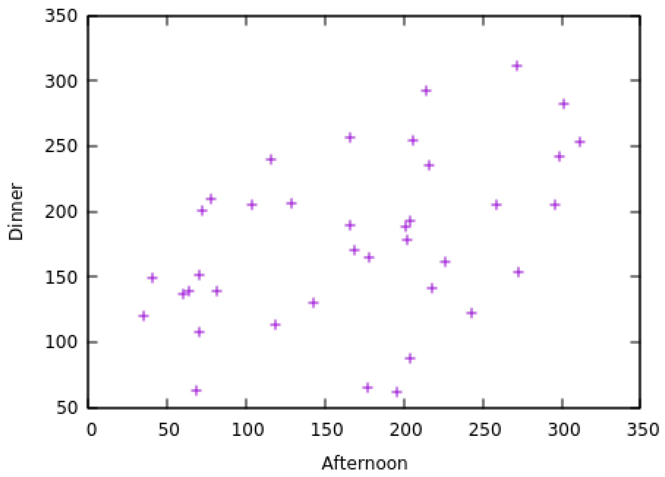
The data received by the prediction module is a tuple composed of the day it was measured, the time of day it was measured and the glucose value. The day is represented as an integer, with one being the value for the day of the first measurement. The time of day is relative to the time the measurement was taken, it can be: before breakfast, before lunch or before dinner. The glucose value is also represented as an integer variable received from the BGM. Scatter-plots of the data obtained from one patient during 28 days can be seen in Figure 1, Figure 2 and Figure 3.
It is possible to see that there isn’t a direct correlation between any pair of measurement and its subsequent measurement. Trying to make a linear regression on this data would result in errors that would not only make incorrect predictions but could also lead to hypoglycemia. Moreover, trying to discretize the data might induce errors, for example, if the data would be discretized in intervals of length 50, it would cause much data of similar values to fall on different classes. This can be easily seen in Figure 1 around the value 100 on the breakfast axis, and in Figure 2 around the value 200 on the Afternoon axis. Separating these data on different classes might induce a loss of precision.
Because of this, a method capable of making accurate predictions for this type of data is needed. Section 3.2 explains the proposed method and why if offers advantages over other traditional methods.
3.2. Prediction Method: Multidimensional Multiscale Forest
Due to the nature of the problem of predicting future glucose values, a new classification algorithm was created named Multidimensional Multiscale Forest (MMF). Most classification methods work only with a finite number of target classes. For such methods to work on data-sets where the prediction variable is on a continuous domain, it is usually required that the data be discretized into a finite number of classes, a process which results in a loss of information that can lead to incorrect decisions by the decision maker supported the system. This can be a problem for applications such as glucose prediction where the output should be on a continuous domain, and the error resulting from the loss of information of the discretization process can lead to situations such as hypoglycemia that are hazardous to human health. In addition, an approach to the problem as a regression has a problem that the data may be organized as different related clusters that may hamper a regression attempt to minimize its error.
For the process of discretization, an expert with extensive knowledge about the application domain is usually necessary to be able to form a good discretization of the data that correctly reflects its application. A bad discretization might lead to incorrect correlations and therefore hamper the classification process. If an expert is not available, or even if one is available but not able to correctly discretize the data, there is no guarantee that the results will be correct or even useful.
The presented method solves such problems by outputting its prediction results as intervals on a continuous domain. This enables the decision maker to have much more precision and less loss of information than if the data were to be discretized.
The presented classification method has a graphical interpretation which resembles Fuzzy ART [26], which has inspired methods that have already been used in other medical areas [27].
For the presented method to work, the following hypothesis needs to hold true: if an instance X is of class Y, then an instance similar to X shall be of a class near Y, where X and Y .
3.3. Classification
The presented method works by creating a forest, which is a list of trees. Each node of the forest represents a decision rule composed of a set of intervals, called attribute intervals, and an interval related to the base interval, called a target interval. Each rule is interpreted as: if a measured value is on the set of attribute intervals, then the value predicted is within the target interval.
The forest is created by receiving as input a parameter and data instances each composed of an array of real numbers, defined as attributes, and a real number associated with such array, defined as its target.
The forest is built from the bottom-up, starting by the leaves of its trees and finishing by its roots. The construction of the forest starts by transforming each instance’s attributes and its target variable into an interval of length centered at its respective value. These form the leaf nodes, each representing a very simple, and overfitting, rule where, if a new data instance has its attributes contained on the intervals, then it is expected that its target will be also contained within the target interval.
The next level of the tree is formed by first sorting the rules created by the median value of its intervals. If every attribute interval of a rule has an intersection with its corresponding intervals from the next rule of the sorted list, then a new rule is formed by merging the attribute and target intervals of both rules. This newly formed rule has assigned as its child nodes the two rules used to form it. Otherwise, if one of the intervals from the two rules of the sorted list doesn’t have an intersection, then a parent rule shall not be formed. This process continues for all rules of the sorted list.
The next levels of the tree are formed by taking the parent rules and repeating the process using them to form new rules. This is repeated at each iteration taking only the parent rules created by the previous iteration. Once no more rules can be created, the algorithm stops.
3.4. Node Analysis
The algorithm outputs a collection of trees, a forest, where each of its nodes is a decision rule. If a classification instance has its parameters contained on the intervals of the parameters intervals of the rule, then it is expected that its target will be also contained on the rule’s target interval. None of the intervals of any node from a tree has an intersection with intervals from nodes of other trees. When classifying a new instance, it is expected that its class will be within the target interval of the rule whose attributes intervals contain the instance’s attributes.
Each node has all the information contained in its child nodes. This creates the following relations between nodes: a parent node has a better generalization but is less accurate than its child nodes. A child node has more accuracy than its parent node but has less generalization.
Another important feature about each node is how reliable it is. Reliability is defined as how many instances were used to form a node, therefore, how much you can trust that a certain node is correct. The reliability of a node can be found by counting how many leaf nodes were used to form it. One node is always more reliable than its child nodes.
It is also possible for a new classification instance to not be contained in any of the rules; in this case, it can be classified with the rule whose intervals are less distant than those of such instance. Another interesting possibility for this case is to not classify the instance and output to the user a warning indicating that this instance is so different than the ones used in training that there is not enough confidence to classify it. This option can be helpful to identify data with errors or outliers, such as on the application of predicting blood glucose, where an incorrect prediction might lead to hypoglycemia.
While discretization is usually needed by most classification methods and may result in loss of information, the Multidimensional Multiscale Forest (MMF) solves this problem by extending the values from the training data into intervals, making it able to form decision rules that, instead of predicting single values, are able to output intervals. This simple change of transforming the data into intervals takes off the necessity of discretizing the data before the classification process starts. Instead, the data is able to be discretized during the formation of classification rules, which enables the formation of multiple layers of different discretization levels without previous knowledge of the application domain required. The algorithm is also applicable in case the target variable is discreet and not continuous. In this case, the classes are simply not transformed into intervals. The process of building the forest is the same as of the continuous case but with one difference—two nodes are only joined if they predict the same class. This makes each rule only predicting only one target class. For this case of classification, it can happen that an instance is within two rules of different classes. If this happens, then the instance is considered to be of the class of the rule that has a smaller volume since it can be considered to be a less general and more precise rule. Thus, the algorithm can be applied for common classification problems with ease.
3.5. Graphical Interpretation
The rules outputted by the MMF are a collection of intervals; therefore, they can easily have a graphical interpretation and be visualized when on low dimensions. If there are two variables used for classification, then the rules can be graphically interpreted as rectangles. If there are three classification variables, then the outputted rules are rectangular prisms and, for problems with more variables, the rules can be interpreted as hyper-rectangles.
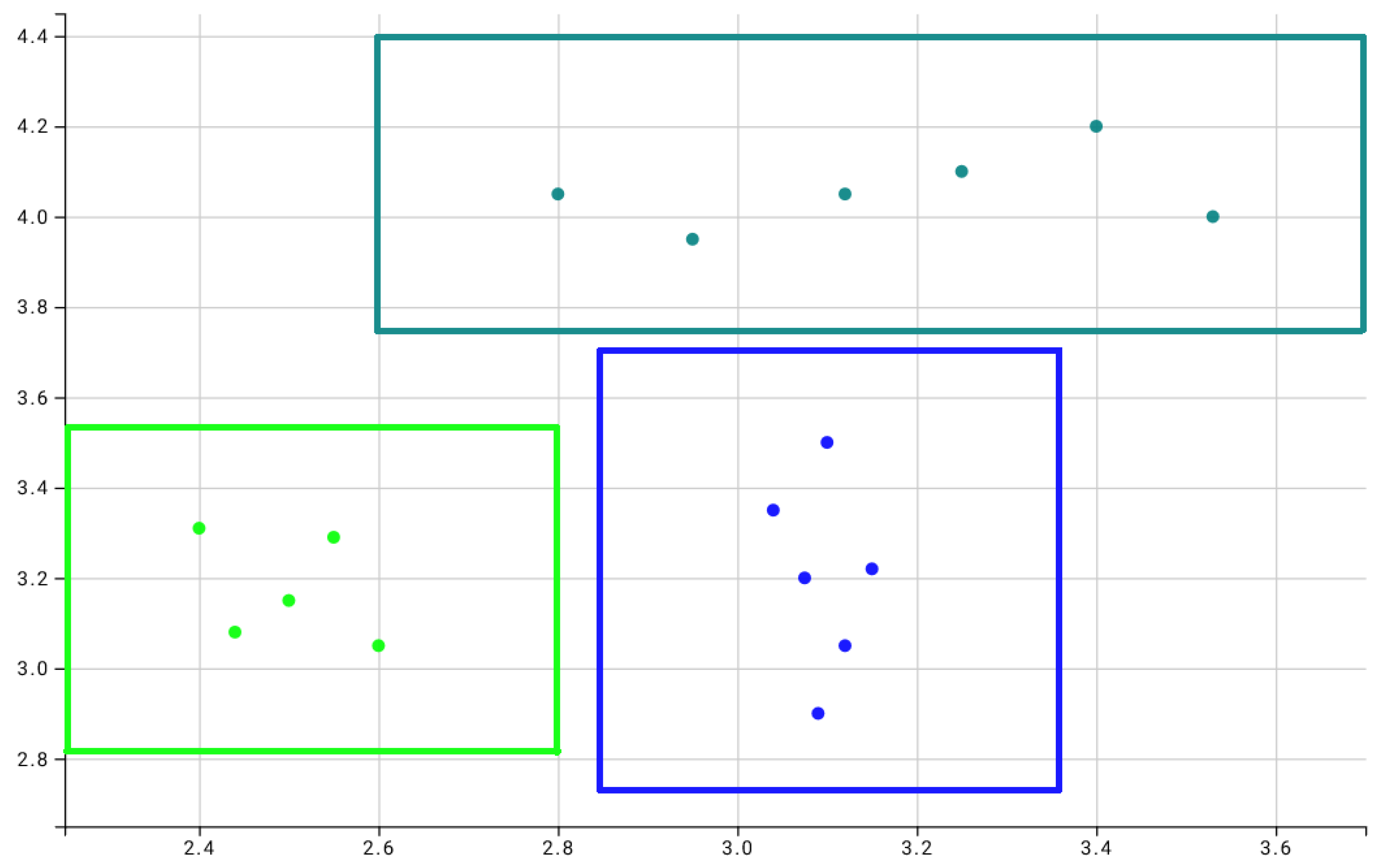
To exemplify this graphical interpretation, Figure 4 shows rules obtained from a test dataset of two dimensions and three classes artificially created to help understand the method. For this problem, only rules with the highest confidence from each tree of the forest—their roots—were considered. Each square represents a different rule, and each class was represented by a different color. The parameter was set as . In total, three rules were found: one for each class.
Any new point that falls inside one of the squares shall be classified as the same class associated with the square. A point that doesn’t fall inside any of the squares can either be classified as the class of the nearest square or be considered an outlier that can’t be classified with the information used in training.
The graphical representation has the rules as squares because the Manhattan norm to measure the distance between a classification instance and the set of intervals used to compose a rule was used. If the Euclidean norm were to be used to measure the distance then instead of rectangles, the rules would be ellipses instead. This possibility of using different norms for distance calculation can be of interest depending on the application of the used data since a different distance norm could lead to a better prediction model.
4. GLUMIS System
The proposed GLUMIS system arose from the need to maintain traceability between diabetes management data to support physicians and health professionals on decision-making regarding patient care as well as characteristics that influence treatment such as eating habits, for example. Figure 5 shows the GLUMIS system architecture with its main components and integration with the REALI system.
In addition to integrating with the REALI tool, the GLUMIS system is capable of integrating data from three different sources: CGMS systems, NGM devices or importing data from glycemic meters (BGM). There is also the possibility of manually entering the glucose level data, the date and time of the measurement. The data is uploaded regularly to the GLUMIS system forming a repository of historical data. A knowledge database is also maintained as decisions are taken, treatment is changed and this information is recorded to support future decisions. The REALI system, the integration feature and the other components of GLUMIS are detailed below.
4.1. REALI System
Initially, the REALI System was designed only to manage the food register. It recorded what had been ingested and when. When requested, the tool generated a synthetic report to be presented to the doctor or nutritionist.
Over time, new needs were being identified and the tool became a system. Developed and offered “as a service” to users and other systems that wish to integrate and use their features.
In the context of GLUMIS: Currently, it provides the user with the management and monitoring of diets in general and can be parameterized depending on the user’s interest. Facing integration with Glumis, for example, it was incorporated with the focus on carbohydrate counting therapy.
Registration Function: Its main purpose is to record the value of carbohydrates ingested each time the patient feeds, in addition to the meal time and the amount of insulin applied to neutralize the carbohydrate.
Greater Control: The tool allows the recording of partial carbohydrate values for each item ingested, maintaining greater control over the type of food ingested and its main properties.
Flexibility: The user can export reports and send them by e-mail.
Integration: Through the integration between the REALI system and the GLUMIS system, the data recorded by the tool become available and compose the data repository, being consumed by the GLUMIS system in the traceability process.
4.2. Glucose Prediction
The prediction method uses a tree created from data taken from a BGM, CGM or even a NGM device, consisting of the glucose value as well as the day and the time period when it was measured (before breakfast, before lunch, etc). The tree outputs rules consisting of two sets, each consisting of: an interval of glucose values and a time period. The rules can be interpreted as: if the patient’s current glucose is on the first set, then it is expected that his future glucose will be on the second set. Each node from the tree has one interval of glucose from one time period and a second interval from another time period, thus each node represents a different rule. An example of a rule can be seen below:
- if (glucose before lunch ) then (glucose before dinner )
The process of creating a tree is bottom-up. Each terminal node is created from a different glucose measure for a given period of time and the measure of another time period that is related to the first one. For example, if it is sought to predict how the patient’s glucose will be before lunch based on measurements done before breakfast, then each node of the tree should have the glucose measurement of before breakfast and the measurement of before lunch, both from the same day. These values are then each transformed into intervals of size where the measured value is in the center.
The nodes are then sorted by the value of their first set. For each pair of neighbour nodes of the same level, a parent node is created if there is an intersection on their first intervals. The intervals of the parent node are the union of the intervals of both child nodes. This process is repeated until no more parent nodes can be created. Figure 6 illustrates the process, highlighted in A, B, and C, in which the prediction tree is created. The numbers in black represent the value of glucose at the time period before breakfast, and red numbers represent blood glucose at before lunch.
An example of raw data collected from a BGM is highlighted in A. Each pair of circles represents measurements taken from the BGM on different days. Circles with black numbers show the value of blood glucose at before breakfast and the circles they point represent the glucose value at the before lunch period from each respective day.
Each measurement from before breakfast with its related before lunch is highlighted in B, as terminal nodes. Each value from A was transformed into an interval using . Each circle is a rule that can be interpreted as: if the a glucose measured at before breakfast is in the black interval, then it will be in the red interval before lunch time.
Finally, the tree after being completely built is highlighted in C. Parent nodes were created by joining the intervals of its child nodes if they had an intersection.
4.3. Reasoner—Analysis of the Decision Tree
The tree is composed of nodes, each representing a rule. While nodes from the top of the tree are more generic rules, with a higher probability of being correct but lacking precision, nodes from the bottom of the tree are the opposite, having more precision but being less likely to be correct.
The search for a rule can be done either manually or automatically. The manual search for a usable rule should start from the top of the tree and descending until a good trade-off between precision and reliability is found. Such decision of what rule has a good trade-off should be made by an expert, either the patient or his physician. Due to the nature of the way the tree is built, every non-terminal node is connected to its two child nodes, the left one always having its center with a smaller value than the center of the right child, making the tree similar to a binary search tree. Thus, the search for a good rule can be done in an efficient way.
An automatic search for a rule can be done by the GLUMIS system. The user inputs his/her latest measured glucose, the time period of the measurement, the time period for the future value to be predicted and how reliable the rule should be. The reliability of a rule is given by the number of terminal nodes used to create it. Next, the GLUMIS system searches for nodes whose first range contains the inputted glycemia with reliability higher than, or equal, to the desired one. Finally, nodes meeting these criteria are displayed, sorted by reliability and by the distance from the center of its first interval to the indicated blood glucose. The Prediction Tree view, presented in the next section, supports this search process.
Advantages of Predicting on a Continuous Domain
The problem of predicting future glucose values differs from traditional classification problems because, while the latter has a discrete number of target classes, glucose values are a continuous domain. Clustering the glucose values into an arbitrary number of classes presents a serious problem in case the patient’s glucose values are clustered around the boundary between two classes. For example, if the class good is defined with values ranging from 80 to 120 and the class medium has values from 121 to 160, then if the measured values vary from 110 to 130, part of them will be classified as good and the other part as medium. This making the prediction difficult since part of his glucose is classified as medium, which would call for a raise on insulin dosage, while the other part part, classified as good, poses a risk of hypoglycemia in case the raise is applied. Because of this problem, most well known classifiers are unable to present rules with enough precision for a change on the treatment since they require the use of discrete target classes.
The main advantage of the proposed method over other classification algorithms lies in its ability to produce rules as intervals. Thus, there is no need for the data to be discretized. This allows for a more realistic overview of the behavior of glucose changes over time. In the example presented above, the algorithm would indicate a range of 110 to 130, which correctly models the patient, thus facilitating a correct treatment change. If a prediction turns out to be wrong, outside the range that it should be, the error is calculated as the distance between the measurement to the interval. If the distance is small, this error may not prove to be a problem for the patient’s health.
A secondary advantage of this method is its ability to only predict glucose from measurements that do not differ by more than the interval chosen during the training. This feature serves as a safety device, especially in applications such as this one which deals with a health application. For example, if a very different measure from those used in training appears, the algorithm will not give a prediction; instead, it will indicate the possible existence of a new glycemic profile of the patient that is safer than giving a prediction with high probability of error, which may result in hypoglycemia.
4.4. Visualization
The GLUMIS system provides three views arranged as a dashboard for the decision maker. They were developed from the JavaScript d3js library. This library was previously used with success in another information system [28].
The Profile View (Figure 7) uses a radar chart to represent different types of information about the glycemic profiles identified through the repository and the knowledge base. Values closer to the center indicate a better profile and thus more adjusted glycemic control. The identification of the profiles takes into account the average glucose measurements for each of the time periods configured by the user. The user can also add tags that describe the profile, for example, “vacation”, or the range of days to which it belongs.
Through interaction elements, it is possible to select a specific profile and highlight the average of each time period, using it to compare with other profiles. In Figure 7, the last identified profiles are displayed and the best one is the Profile C associated with the last three months.
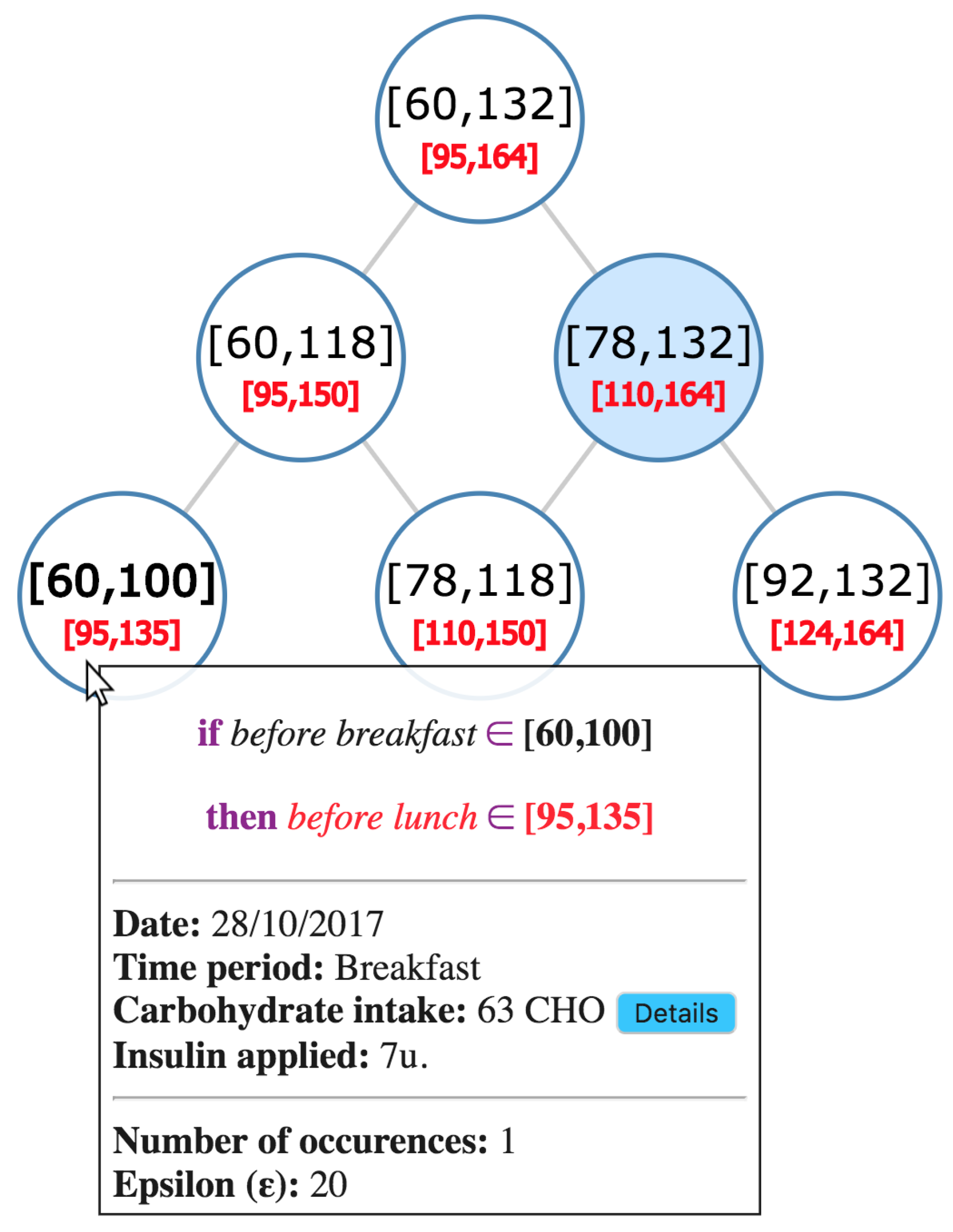
The Prediction Tree View (Figure 8) uses a graph to represent, at each node, the information about the identified rule and the analyzes made by the Reasoner. This view is the user interface to configure the prediction tree creation. The user can define, for example, the epsilon value and the number of measurements to be considered.
Through interaction elements, it is possible to select the rule that will guide the decision-making process. In addition, information such as the rule outlining the measurement intervals, the number of occurrences considered to generate the rule and the epsilon value considered can be obtained, as well as the date of measurement and which time period is associated. The dosage of insulin applied and the amount of total carbohydrate ingested are also highlighted, with the possibility of showing a detailed description. In the Figure 8, the rules and the reasoner analysis are displayed for the example given in the previous subsection.
The Historical Traceability View (Figure 9) uses a combined bar and line chart to represent traceability information between glucose measurements, carbohydrate intake, and insulin doses.
The view is generated after the user selects a range of days and a time period to be analyzed. As shown in Figure 9, the line represents the evolution of glucose measurements in the chosen period. The line color is associated with the measurements mean against a normality scale for glucose levels. This scale can be changed by the physician or health care professional, although it has a set pattern. Bars represent the amounts of insulin and carbohydrate, respectively.
Through interaction elements, it is possible to obtain contextual information such as the average glucose measurements in the period, with a reference to the range of values considered “normal”, the average carbohydrate intake in the period, as well as the average insulin applied. The ratio of carbohydrate to insulin is also highlighted. Regarding the current occurrence under analysis, the date of measurement, the insulin dosage applied and the amount of carbohydrate ingested are also highlighted, with the possibility of showing a detailed description in addition to glucose measurement, colored according to the normality scale and how much it varied from the average. This feature allows the analysis of variability in glycemic control.
5. Evaluation
This section presents the experimental study conducted. According to the Goal/Question/Metric approach (GQM) [29], the goal can be stated as: “Analyze the GLUMIS system in order to verify the feasibility of use with respect to the task of interpreting the views and rules from the point of view of patients and physicians in the context of diabetes management through a decision support system”.
In this sense, two questions were defined to be answered by the participants, for each visualization of the system. In Question 1 (Q1), the participant should assess the degree of comprehension associated with the visualization and information presented. For this, they should use a scale where 1 indicates very difficult and 5 indicates very easy. In Question 2 (Q2), if the participant agreed that the view supported the understanding of the rules and the analysis made by Reasoner. Using for this a scale where 1 indicates totally disagree and 5 indicates totally agree.
The experiment was proposed based on a set of real data collected from two consecutive months taken from measurements done by BGM and CGMS. A database was considered with the glucose measurements of a patient that agreed to partake on this study. The time periods used were before breakfast, before lunch and before dinner and for each one was collected at least 25 measurements.
This experiment included 10 participants: nine patients and one specialist. After filling out a form characterization, it was observed that the patients were between 21 and 62 years old, most of them with diabetes mellitus type 1 and 2 with diabetes mellitus type 2. Among patients with type 2 diabetes, one use BGM and the other a CGMS. Among patients with type 1 diabetes, three stated that they use a CGMS and the other four make use of a BGM as a glucose meter. For characterization reasons, two questions were answered by the 10 participants. It was possible to identify that, with respect to the participant’s ease of dealing with new technologies, of interviewees said they had a very high level of ease, another said they had high ease, regular and indicate that they have low ease in dealing with new technologies. In addition, about the ease of interpreting charts, of respondents said that they had a very high level of ease, said they had high ease, say they have a regular facility, and say they have low ease in interpreting charts. This diversity shows the GLUMIS system’s ability to assist people with different skill levels in dealing with new technologies or in interpreting charts.
The participants were submitted to online training where the preliminary doubts were answered. Then, during the conduction of the experiment, the evaluation environment and participants were observed by the authors of this study. In addition, the participants were encouraged to comment and describe their impressions.
During the analysis and decision-making process, the Prediction Tree View was displayed with the rules identified. In addition, the Profile View and the Historical Traceability View were presented, showing the new glycemic profiles identified and the historical traceability data between diet information and carbohydrates ingested, the amount of insulin applied and glucose measurements through time. Through interaction elements, the visualizations were analyzed by a specialist to find relevant rules for a change on the patient’s treatment.
The GLUMIS system was able to provide many interesting rules which helped to provide valuable information about each patient. One patient’s data for the glucose prediction test was used, data was collected from 28 days with measurements from before breakfast, before lunch, afternoon break and before dinner. The MMF algorithm was used to process this data and create a forest, which showed the relations of different time periods; the outputted forest was analyzed by a specialist to find interesting rules capable of aiding the patient’s treatment. Some interesting rules found with the data of one patient are shown bellow:
- Rule 1: if glucose before breakfast , then glucose at afternoon break in
- Rule 2: if glucose at afternoon break , then glucose before dinner
- Rule 3: if glucose before dinner , then glucose before breakfast of the next day
The values of were chosen by the specialist taking into account the variation that can happen by two consecutive measurements done by the same BGM, the maximum value of 15 was set by the specialist as an acceptable variation. By observing the results showed by the visualization module, the rules showed above were found by using the following values of : For the first rule, it was found was with set as 5 for the time period before breakfast, 5 for afternoon break. For the second rule, it was found with 12 for afternoon break and 9 for before dinner. For the third rule, it was found with 9 for dinner and 5 for before breakfast.
These three rules were able to aid the specialist on changing this specific patient’s treatment by providing a more precise view of his condition. Below is the reasoner’s interpretation of the rules, why they are relevant in this context, and the association with diet data and insulin dosages.
Rule 1 indicates that, if there is a hypoglycemia before breakfast, then the glucose will be high in the afternoon break. By identifying the patient’s glycemic profile and eating habits, it was possible to identify that, due to the low glucose in the morning, the patient increased carbohydrate intake during lunch and decreased the dose of insulin. This resulted in an increase of glucose at after lunch.
Rule 2 indicates that if glucose is low after lunch, then glucose may show a normal value before dinner. This fact shows signs that the current dose of insulin and food intake, in this case, are already adjusted.
Rule 3 indicates that, if glucose is high before dinner, then glucose may be low by the morning of the next day. This fact showed that the proportion of insulin ingested at night was high resulting in hypoglycemia in the next morning.
These rules were able to provide valuable information to improve patient glucose control. In face of visualizations and Rule 1 analysis, the physician (specialist) asked the patient to correct hypoglycemia during breakfast and to maintain the proportion of insulin per carbohydrate eaten at lunch. By Rule 2, insulin doses should be maintained. Rule 3 prompted the physician to ask the patient to correct hyperglycemia at dinner and reduced the proportion of insulin applied per gram of ingested carbohydrate.
Results and Lessons Learned
Responses and considerations were collected and organized. Table 1 shows the averages received by each visualization in the Q1 and Q2 survey questions.
The results obtained by the questionnaire responses indicate that, in relation to Q1, the participants considered the visualizations to be easy or very easy to understand. Regarding Q2, the results indicate that the participants agreed or fully agreed that the “Profile View” and “Prediction Tree View” supported the understanding of the rules and the analysis made by the Reasoner. Considering that the average of the ratings received is higher than 3 (three), thus above the area of indifference proposed by the scale, then, according to the participants, the “Historical Traceability View” also supports the understanding of the rules and the analysis made by Reasoner.
Through a textual report that each participant could write at the end of the experiment, it was possible to extract some extra information and learn some lessons.
Some participants considered that “Prediction Tree View” was very simple, even though it received a high rating on Q1. According to the reports, it could be improved to show, for example, the path that originated the rule in automated research.
The textual report of one of the participants suggested that the system offer to the user the possibility of defining an ideal or desirable profile. Thus, if the current profile approaches that established as desirable, then the physician and the patient are reported and the treatment may be altered or the frequency of medical follow-up.
According to reports from four participants, there may have been redundancy between the information shown by the “Prediction Tree View” and the “Historical Traceability View”. For this reason, these participants classified the “Historical Traceability View” that would be indifferent in understanding the rules.
In fact, both views present insulin-related data and ingested carbohydrates. Thus, the participant did not realize the need to also use the contextual data, of the other days, shown by the “Historical Traceability View”. However, the “Prediction Tree View” and the “Historical Traceability View” have very different objectives: the first provides a punctual notion of the values and the second traces a historical parallel from three types of data: insulin, carbohydrate and value glycemic index. A possible explanation for this phenomenon is related to the reduced universe of data used that did not allow the participant to visually differentiate the purpose of each visualization. Familiarity with new technologies and visual metaphors may be another explanation.
As threats to validity, we can mention the reduced number of participants containing 1 specialist. To minimize the effect of this threat, it was possible to observe that the participants can represent different profiles.
Throughout the experiment, the generated database had balanced amounts of measurements of glucose, insulin and carbohydrates ingested for the periods of time considered. The application of this study on databases concentrated in specific periods of the day can reach different results.
6. Conclusions
It is common for patients with diabetes to periodically measure their glucose level as part of their treatment. The presented system, GLUMIS, is able to predict future glucose values based on measurements obtained from a Blood Glucose Meter (BGM), or a Continuous Glucose Measurement System (CGMS), or even a Non-invasive Glucose Monitoring (NGM) device. Prediction produces rules that would otherwise not be found by traditional methods of glucose monitoring.
The GLUMIS system was not designed as a recommendation system with the best treatment option for the analyzed patient and, therefore, it is not intended to replace the health professional or the physician. Rather, it provides users with information that is enriched by visualizations that help create a big picture about the treatment they have adopted. As for the patient using the GLUMIS system, a means of monitoring and understanding the treatment itself is offered.
It is worth mentioning that this paper is an extended version and one of the objectives was to explain, for the first time, the application of the innovative algorithm created for prediction in the GLUMIS system. This algorithm innovates by not needing the data to be discretized by a specialist by transforming single values into intervals, being able to output rules as intervals capable of a good generalization and precision. It also is able to detect outliers and not make predictions with low confidence lowering the risk of wrong predictions. In this context, the GLUMIS system served as a case study for the evaluation of technical aspects, such as accuracy, of the new algorithm.
Among the contributions of this study it is possible to cite the GLUMIS system itself, the method of prediction applied, the creation of a patient’s own knowledge database and the possibility of maintaining traceability between different information, at the same time as it stores the new decisions made at every change in treatment. This helps in obtaining a historical view of the patient as well as a future perspective.
An experimental study was carried out to analyze the system, prediction method and visualizations in a decision-making context and resulted in interesting rules that have helped to improve patient care.
There is future work to seek new partnerships and conduct new experiments in order to draw a parallel between the use of the system by patients with type 1 diabetes and type 2 patients—in addition to making improvements for the system to become a recommendation system, indicating possible changes in the insulin application schedule to favor glycemic control.
Author Contributions
Formal Analysis, R.M.G.; Investigation, C.A.S.L.; Software, C.A.S.L.; Validation, R.M.G.; Visualization, R.M.G. In other words, C.A.S.L. envisioned the system and worked on the visualization and support system. R.M.G. developed the prediction algorithm and applied it to glucose prediction.
Funding
This study was financed in part by the Coordenação de Aperfeiçoamento de Pessoal de Nível Superior-Brasil (CAPES)-Finance Code 001.
Conflicts of Interest
The authors declare no conflict of interest. The founding sponsors had no role in the design of the study; in the collection, analyses, or interpretation of data; in the writing of the manuscript, and in the decision to publish the results.
References
- American Diabetes Association. Diagnosis and classification of diabetes mellitus. Diabetes Care 2014, 37, S81–S90. [Google Scholar] [CrossRef] [PubMed]
- Rowley, W.R.; Bezold, C.; Arikan, Y.; Byrne, E.; Krohe, S. Diabetes 2030: Insights from Yesterday, Today, and Future Trends. Popul. Health Manag. 2017, 20, 6–12. [Google Scholar] [CrossRef] [PubMed] [Green Version]
- Rahbar, S. The discovery of glycated hemoglobin: A major event in the study of nonenzymatic chemistry in biological systems. Ann. N. Y. Acad. Sci. 2005, 1043, 9–19. [Google Scholar] [CrossRef] [PubMed]
- Aronson, D. Hyperglycemia and the pathobiology of diabetic complications. In Cardiovascular Diabetology: Clinical, Metabolic and Inflammatory Facets; Karger Publishers: Basel, Switzerland, 2008; Volume 45, pp. 1–16. [Google Scholar]
- Zhang, P.; Zhang, X.; Brown, J.; Vistisen, D.; Sicree, R.; Shaw, J.; Nichols, G. Global healthcare expenditure on diabetes for 2010 and 2030. Diabetes Res. Clin. Pract. 2010, 87, 293–301. [Google Scholar] [CrossRef] [PubMed]
- Whiting, D.R.; Guariguata, L.; Weil, C.; Shaw, J. IDF diabetes atlas: Global estimates of the prevalence of diabetes for 2011 and 2030. Diabetes Res. Clin. Pract. 2011, 94, 311–321. [Google Scholar] [CrossRef] [PubMed]
- Guariguata, L.; Whiting, D.; Weil, C.; Unwin, N. The International Diabetes Federation diabetes atlas methodology for estimating global and national prevalence of diabetes in adults. Diabetes Res. Clin. Pract. 2011, 94, 322–332. [Google Scholar] [CrossRef]
- Ogurtsova, K.; da Rocha Fernandes, J.; Huang, Y.; Linnenkamp, U.; Guariguata, L.; Cho, N.; Cavan, D.; Shaw, J.; Makaroff, L. IDF Diabetes Atlas: Global estimates for the prevalence of diabetes for 2015 and 2040. Diabetes Res. Clin. Pract. 2017, 128, 40–50. [Google Scholar] [CrossRef]
- Clarke, S.F.; Foster, J.R. A history of blood glucose meters and their role in self-monitoring of diabetes mellitus. Br. J. Biomed. Sci. 2012, 69, 83–93. [Google Scholar] [CrossRef]
- Vashist, S.K.; Zheng, D.; Al-Rubeaan, K.; Luong, J.H.; Sheu, F.S. Technology behind commercial devices for blood glucose monitoring in diabetes management: A review. Anal. Chim. Acta 2011, 703, 124–136. [Google Scholar] [CrossRef]
- Vashist, S.K. Non-invasive glucose monitoring technology in diabetes management: A review. Anal. Chim. Acta 2012, 750, 16–27. [Google Scholar] [CrossRef]
- Lin, T.; Mayzel, Y.; Bahartan, K. The accuracy of a non-invasive glucose monitoring device does not depend on clinical characteristics of people with type 2 diabetes mellitus. J. Drug Assess. 2018, 7, 1–7. [Google Scholar] [CrossRef] [PubMed] [Green Version]
- Guillod, L.; Comte-Perret, S.; Monbaron, D.; Gaillard, R.C.; Ruiz, J. Nocturnal hypoglycemias in type 1 diabetic patients: What we can learn with continuous glucose monitoring? Diabetes Metab. 2007, 33, 360–365. [Google Scholar] [CrossRef] [PubMed]
- Maia, F.; Araujo, L. Effect of continuous glucose monitoring system (CGMS) to detect postprandial hyperglycemia and unrecognized hypoglycemia in type 1 diabetic patients. Diabetes Res. Clin. Pract. 2007, 75, 30–34. [Google Scholar] [CrossRef] [PubMed]
- Facchinetti, A. Continuous Glucose Monitoring Sensors: Past, Present and Future Algorithmic Challenges. Sensors 2016, 16, 2093. [Google Scholar] [CrossRef] [PubMed]
- Vashist, S.K. Continuous glucose monitoring systems: A review. Diagnostics 2013, 3, 385–412. [Google Scholar] [CrossRef] [PubMed]
- Guerci, B.; Floriot, M.; Böhme, P.; Durain, D.; Benichou, M.; Jellimann, S.; Drouin, P. Clinical performance of CGMS in type 1 diabetic patients treated by continuous subcutaneous insulin infusion using insulin analogs. Diabetes Care 2003, 26, 582–589. [Google Scholar] [CrossRef] [PubMed]
- Spence, R. Information Visualization: Design for Interaction; Pearson/Prentice Hall: Upper Saddle River, NJ, USA, 2007. [Google Scholar]
- Ainsworth, S. The functions of multiple representations. Comput. Educ. 1999, 33, 131–152. [Google Scholar] [CrossRef]
- Vazeou, A. Continuous blood glucose monitoring in diabetes treatment. Diabetes Res. Clin. Pract. 2011, 93, S125–S130. [Google Scholar] [CrossRef]
- Sola-Gazagnes, A.; Vigeral, C. Emergent technologies applied to diabetes: What do we need to integrate continuous glucose monitoring into daily practice? Where the long-term use of continuous glucose monitoring stands in 2011. Diabetes Metab. 2011, 37, S65–S70. [Google Scholar] [CrossRef]
- Moser, E.G.; Morris, A.A.; Garg, S.K. Emerging diabetes therapies and technologies. Diabetes Res. Clin. Pract. 2012, 97, 16–26. [Google Scholar] [CrossRef]
- Lélis, C.A.S.; Motta, R. A Complete Diabetes Management and Care System. In Information Technology-New Generations; Springer: Berlin, Germany, 2018; pp. 651–658. [Google Scholar]
- Bondia, J.; Tarín, C.; García-Gabin, W.; Esteve, E.; Fernández-Real, J.M.; Ricart, W.; Vehí, J. Using support vector machines to detect therapeutically incorrect measurements by the MiniMed CGMS®. J. Diabetes Sci. Technol. 2008, 2, 622–629. [Google Scholar] [CrossRef] [PubMed]
- Eljil, K.S.; Qadah, G.; Pasquier, M. Predicting hypoglycemia in diabetic patients using data mining techniques. In Proceedings of the 2013 9th International Conference on Innovations in Information Technology, Al Ain, UAE, 17–19 March 2013; pp. 130–135. [Google Scholar]
- Carpenter, G.; Grossberg, S.; Rosen, D. Fuzzy ART: Fast Stable Learning and Categorization of Analog Patterns by an Adaptive Resonance System. Neural Netw. 1991, 4, 759–771. [Google Scholar] [CrossRef]
- Xu, R.; Anagnostopoulos, G.; Wunsch, D. Multiclass Cancer Classification Using Semisupervised Ellipsoid ARTMAP and Particle Swarm Optimization with Gene Expression Data. IEEE/ACM Trans. Comput. Biol. Bioinform. 2007, 4, 65–77. [Google Scholar] [CrossRef] [PubMed]
- Lélis, C.A.; Miguel, M.A.; Araújo, M.A.P.; David, J.M.N.; Braga, R. AD-Reputation: A Reputation-Based Approach to Support Effort Estimation. In Information Technology-New Generations; Springer: Berlin, Germany, 2018; pp. 621–626. [Google Scholar]
- Basili, V.R.; Weiss, D.M. A Methodology for Collecting Valid Software Engineering Data. IEEE Trans. Softw. Eng. 1984, SE-10, 728–738. [Google Scholar] [CrossRef]
Figure 1.
Scatter plot of a measurement at breakfast and in the afternoon on the same day.

Figure 2.
Scatter plot of a measurement in the afternoon and at dinner on the same day.

Figure 3.
Scatter plot of a measurement at dinner and at breakfast on the next day.

Figure 4.
Rules found for a sample dataset. Each color represents one of three different classes. Each square represents a classification rule associated with its class’s color.
Figure 4.
Rules found for a sample dataset. Each color represents one of three different classes. Each square represents a classification rule associated with its class’s color.

Figure 5.
GLUMIS architecture.

Figure 6.
Process to create the tree. Sub-Figure A represents raw data. Sub-Figure B represents data after being transformed into intervals. Sub-Figure C shows the tree after being built by the algorithm.
Figure 6.
Process to create the tree. Sub-Figure A represents raw data. Sub-Figure B represents data after being transformed into intervals. Sub-Figure C shows the tree after being built by the algorithm.

Figure 7.
Profile view.

Figure 8.
Prediction tree view.

Figure 9.
Historical traceability view.


Table 1.
Research questions average.
| Visualization | Q1 Average | Q2 Average |
|---|---|---|
| Prediction Tree View | 4.6 | 4.8 |
| Profile View | 4.6 | 4.4 |
| Historical Traceability View | 4.8 | 3.8 |
© 2018 by the authors. Licensee MDPI, Basel, Switzerland. This article is an open access article distributed under the terms and conditions of the Creative Commons Attribution (CC BY) license (http://creativecommons.org/licenses/by/4.0/).
Share and Cite
MDPI and ACS Style
Lélis, C.A.S.; Motta Goulart, R. A Diabetes Management Information System with Glucose Prediction. Information 2018, 9, 319. https://doi.org/10.3390/info9120319
AMA Style
Lélis CAS, Motta Goulart R. A Diabetes Management Information System with Glucose Prediction. Information. 2018; 9(12):319. https://doi.org/10.3390/info9120319
Chicago/Turabian StyleLélis, Cláudio Augusto Silveira, and Renan Motta Goulart. 2018. "A Diabetes Management Information System with Glucose Prediction" Information 9, no. 12: 319. https://doi.org/10.3390/info9120319
Note that from the first issue of 2016, this journal uses article numbers instead of page numbers. See further details here.