Finding Group-Based Skyline over a Data Stream in the Sensor Network

Abstract

Along with the application of the sensor network, there will be large amount of dynamic data coming from sensors. How to dig the useful information from such data is significant. Skyline query is aiming to identify the interesting points from a large dataset. The group-based skyline query is to find the outstanding Pareto Optimal groups which cannot be g-dominated by any other groups with the group same size. However, the existing algorithms of group-based skyline (G-Skyline) focus on the static data set, how to conduct advanced research on data stream remains an open problem at large. In this paper, we propose the group-based skyline query over the data stream. In order to compute G-Skyline efficiently, we present a sharing strategy, and based on which we propose two algorithms to efficiently compute the G-Skyline over the data stream: the point-arriving algorithm and the point-expiring algorithm. In our experiments, three synthetic data sets are used to test our algorithms; the experiments results show that our algorithms perform efficiently over a data stream.

1. Introduction

The Internet of Things is the inter-networking of physical devices, vehicles and other items embedded with different information sensors. These sensors can collect much data from the terminals. The most importance is how to dig useful information from these mass data for special purpose.

As one of the important means of multi-decision making, skyline query plays an important role in the applications of sensor network, data mining and so on. The skyline of a data set includes all the points which are not worse than any other points. Given a data set D with d-dimension, every point q can be written as (q[1], q[2], …, q[d]) where q[i] is the ith attribute value of q. Assume that there are two points p = (p[1], p[2], …, p[d]) and q = (q[1], q[2], …, q[d]) in R^d, we say q dominates p, if q[j] ≤ p[j] for each j and there is at least one j(1 ≤ j ≤ d), q[j] < p[j]. The skyline of D consists of all the points which are not dominated by any other points in D. So the skyline query identifies all the best individual points.

For example, in the application of forest fires monitoring, the sensor nodes can perceive nearby temperature, humidity and smoke density. When the fire happens, the nearby temperature will increase and the humidity will decrease, and the nearby sensors can perceive these changes. So a wireless sensor network can be arranged to monitor fire. As shown in Figure 1a, there is a data set D = {p₁, p₂, …, p₁₁}, and each point represents a sensor node with two attributes: the inverse-temperature and the humidity. Doing the skyline query on the sensor nodes can return the skyline points with lower inverse-temperature and lower humidity, as shown in Figure 1b, and these indicate the dangerous areas. We find that the point p₆ dominates point p₃ because the inverse-temperature and humidity of p₆ are smaller than that of p₃. The skyline of the dataset D consists of p₁, p₆ and p₁₁. Therefore, the firemen can quickly identify these dangerous areas and take an earlier action.

However, the fire forces are limited and we cannot check each area at the same time, so if we intend to select 2 areas to examine, the traditional skyline query cannot return what we want directly. In order to solve such problem in a better way, the group-based skyline query was proposed. The group-based skyline (G-Skyline for short) query is to identify the best groups not g-dominated by any other groups with the same group size, and paper [1] proposed two algorithms for computing G-Skyline. Different from the traditional skyline, the G-Skyline presents much more useful information in more complexity phenomena such as sensor network, multi-decision and data mining. In the above example, the G-Skyline groups with 2 points include {p₁, p₆}, {p₁, p₁₁}, {p₆, p₁₁}, {p₆, p₃}, {p₁₁, p₈}, {p₁₁, p₁₀}, then the fire force could consider selecting one group from the result.

Although the G-Skyline is very useful, the existing algorithms focus on the static data set. In fact, in the wireless network, each sensor node maybe sends the perceived data to receiver at intervals, and the environmental intrusion or node-fault maybe affects the perceived data to be send, therefore the data received is dynamic. We can regard these dynamic data as data stream. In the data stream, each data has its life cycle which is from its arriving time to its expiring time, and it is only effective in its life cycle, so when a data arrives or expires, the current active data set will changes. Based on the data in Figure 1, we give an example of data stream in Figure 2. At first, there are 3 points {p₁, p₂, p₃}, at moment t, a new point p₄ arrives, the active points are {p₁, p₂, p₃, p₄}, and at moment 2t, an old point p₂ expires, now the active points are {p₁, p₃, p₄}. With the dataset changing, the groups set will also change, for example, at first, the groups with 2 points are {p₁p₂, p₂p₃, p₁p₃}, when the point p₄ arrives, the groups with 2 points change to {p₁p₂, p₁p₃, p₁p₄, p₂p₃, p₂p₄, p₃p₄}, the groups containing p₄ appear, when the point p₂ expires, the groups with 2 points change to {p₁p₃, p₁p₄, p₃p₄}, the groups containing p₂ are removed.

With the groups set changing, the corresponding G-Skyline maybe also changes. For example, at first, the G-Skyline groups are {p₁p₃, p₂p₃} because p₁p₂ is dominated by p₂p₃, while p₁p₃ and p₂p₃ are not be g-dominated by any other groups. When p₄ arrives, the G-Skyline groups are {p₁p₃, p₁p₄, p₃p₄, p₂p₃}, we can see that the new point arriving affect the G-Skyline result. When p₂ expires, the G-Skyline changes to {p₁p₃, p₁p₄, p₃p₄}, the result shows the old point expiring affect the G-Skyline too. So in order to keep the G-Skyline effective all the time in the data stream, we should update the G-Skyline when the new data arrives or an old data expires.

The naive method to find the G-Skyline over a data stream is to use the existing algorithm PWise in paper [1] directly when the data set changes. However, the data may change quickly in the data stream, under this circumstance, repeating PWise computation for the whole data set will need much time cost and much redundant computation. Because when a new data arrives or an old data expires, some G-Skyline groups may not change their status. For example, in Figure 2, the groups p₁p₃ and p₂p₃ are G-Skyline groups at the moment t and 2t. That is to say, in a data stream, when a point arrives or expires, we do not compute all the groups again. In this paper, we present two algorithms to efficiently find G-Skyline over a data stream in the sensor network. The point-arriving-algorithm can compute the new G-Skyline when a new point arrives, and the point-expire-algorithm will get the new G-Skyline result while an old point expires. In order to improve this two algorithms effectively, we present some pruning theorems to remove the groups which will not affect the new G-Skyline.

We summarize our main contributions in brief as follows.

• We present the problem of finding the G-Skyline with k points over a data stream in the sensor network. This query will provide much more useful information.
• We present a sharing strategy to make us compute the new G-Skyline based on the existing result. According to the pruning theorems, lots of groups will be pruned without computation.
• We propose two algorithms to compute the new G-Skyline over a data stream.
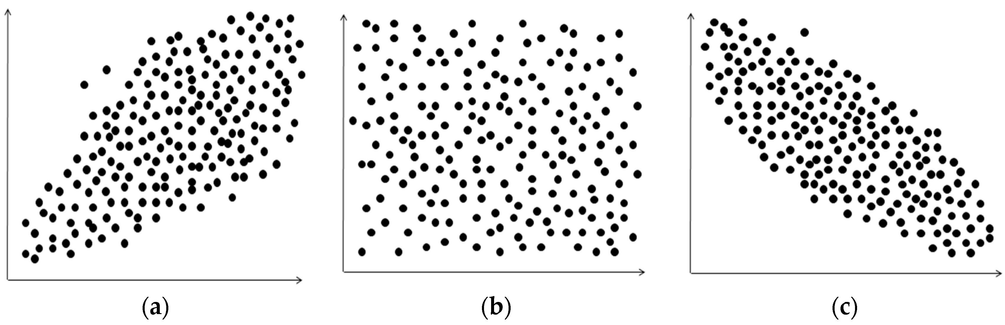
• The experiments are performed based on three kinds of synthetic datasets.

2. Related Work

Since Borzsonyi et al. [2] proposed the skyline operatorin 2001, the skyline has been researched in many filed, and there are many algorithms of skyline have been proposed for different problems. Next, we describe the related work of skyline query.

BNL algorithm and D&C algorithm were proposed in paper [2]. BNL computed the skyline by scanning the whole data set and maintaining a candidate set, D&C returned the final skyline set by computing each sub-set skyline. Paper [3] introduced the algorithm SFS to return the skylineafter all the data being sorted according to the monotone function. Tanet al. [4] firstly firstly mapped each tuple to a m-bit vector, then got the skyline by computing the vectors, but this algorithm was only suitable for the static data set. Kossmann et al. [5] introduced NN algorithm returned the skyline result by filtering the nearest neighbor points. BBS managed the data set by R-tree, and only the nodes containing result points would be visited.

In addition, there are some new skyline algorithms for the specific environment. The sub-space skyline [6,7,8,9] can compute the skyline by dividing the data set to some sub-space. k-dominant skyline [10,11] can return the points which are not k-dominated by any other points, it can find much more potential information. Top-k skyline [12,13,14,15,16] will find the points ranking in the top k position, this algorithm was only suitable for the query within a set limit in volume. In recent years, the skyline query on uncertain data has been studied, in this query, a threshold q was given at first, then the points whose probabilities are larger than q would be returned as probabilistic skyline [17,18,19]. Paper [20,21] introduced the MapReduce technology to compute the skyline efficiently. Paper [22] firstly proposed the skyline query in a data stream, the data in the sliding window were managed in R-tree, and the skyline set was maintained by the interval tree. Paper [23] presented algorithm LOOK-OUT to compute skyline in a data stream. In paper [24], the data in the sliding window were managed based on a multi-layer grid structure. Paper [25] proposed a parallel algorithm for window-based skyline targeting multicores.

The most related to our problem are [26,27,28,29,30,31,32,33]. Paper [26] returned the top-k composition skyline, however, this paper did not propose the composition skyline formally. Im et al., Zhang et al. and Chung et al. [27,28,29] defined and researched the group skyline query, they calculated the value of the same attribute of k points to form a group, then compared the dominance relation between the groups using the traditional dominance. The calculate functions commonly used in these work were some aggregate functions, such as, SUM, MAX, and MIN. H Zhu et al. revealed characteristics of existing algorithms of group skyline and proposed a novel multi-core algorithm to compute group skyline [30,31]. Paper [32] defined the group dominance concept based on uncertain data. In fact, which aggregate function should be used in practical application is difficult to select, so paper [1] proposed the Pareto optimal groups and group-base skyline, which can return all the Pareto optimal solutions. Paper [33] proposed an efficient skyline group algorithm based on the algorithms in paper [27,28] in a data stream, but it was not suitable for the Pareto Optimal groups.

3. Preparations

In this section, we will present the foundation work, including the relevant definitions, basic theorems and the G-Skyline algorithm in static data that will be used in our paper, then we propose our problem.

3.1. Definitions and Theorems

Definition 1.

(Skyline) There are two different points p and q coming from the same data set D, we can say q dominates p, denoted by q $\prec$ p, if q[j] ≤ p[j] for every j (1 ≤ j ≤ d) and at least one j, q[j] < p[j] (1 ≤ j ≤ d), where p[j] is the jth attribute value. The skyline consist of all the points which are not dominated by any other point in D.

Definition 2.

(G-Dominante) Given a data set D, there are two different groups G₁ = {p₁, p₂, …, p_k} and G₂ = {p₁’, p₂’,…, p_k’ }, where each point coming from D, we can say G₁g-dominates G₂, if two arrays with k points for G₁ and G₂ are found, G₁ = {p_n1, p_n2, …, p_nk}and G₂ = {p_m1’, p_m2’, …, p_mk’}, and p_ni ≤ p_mi for each i (1 ≤ i ≤ k) and at least one i, p_ni dominates p_mi.

Definition 3.

G-Skyline) The G-Skyline consist of all the groups with k points which are not g-dominated by any other group with the same size.

Example 1.

The G-Skyline is different from skyline, and it is also not same as skyline groups [24,25,26]. We take the data in Figure 1 as an example. Let G₁ = {p₆, p₈, p₁₁} and G₂ = {p₂, p₃, p₁₀}, we can say G₁g-dominates G₂ because there are two arrays G₁ = {p₆, p₁₁, p₈} and G₂ = {p₃, p₁₀, p₂} such that p₆ $\prec$ p₃, p₁₁ $\prec$ p₁₀, and p₈ $\prec$ p₂. So G₂ is not the G-Skyline group, but G₁ belongs to G-Skyline because there is no other groups g-dominates G₁ with the same size.

Definition 4.

(Skyline Layers) The data set D can be divided to some layers, the layer_i is composed by skyline points of (D-${\displaystyle {\cup }_{j=1}^{i-1}laye{r}_j}$ ), such as layer_i=skyline (D-${\displaystyle {\cup }_{j=1}^{i-1}laye{r}_j}$) which is computed recursively until all the points of D are in layers, where layer₁ is the traditional skyline of D.

Theorem 1.

Given a data set D and the group size k, each point of G-Skyline groups must be in the first k skyline layers (see [1]).

Theorem 2.

If there is a non G-Skyline group G with k points, when another point from G’s tail set is added to it, this new group with k+1 point also does not belong to the G-Skyline (see [1]).

Theorem 3.

For each point p of a G-Skyline group G, all of p’s parents must be in G too (see [1]).

3.2. Algorithm in Static Data

To compute the G-Skyline groups with k points from the given n points, the crude method is to enumerate all the $\left(\underset{k}{\overset{n}{}}\right)$ groups, and then do the query based on the g-dominance. Obviously doing it like this needs much time cost and storage cost, so paper [1] proposes the PWise (Point-Wise) algorithm to efficiently compute the G-Skyline groups. Next, we introduce this algorithm in brief.

(1)

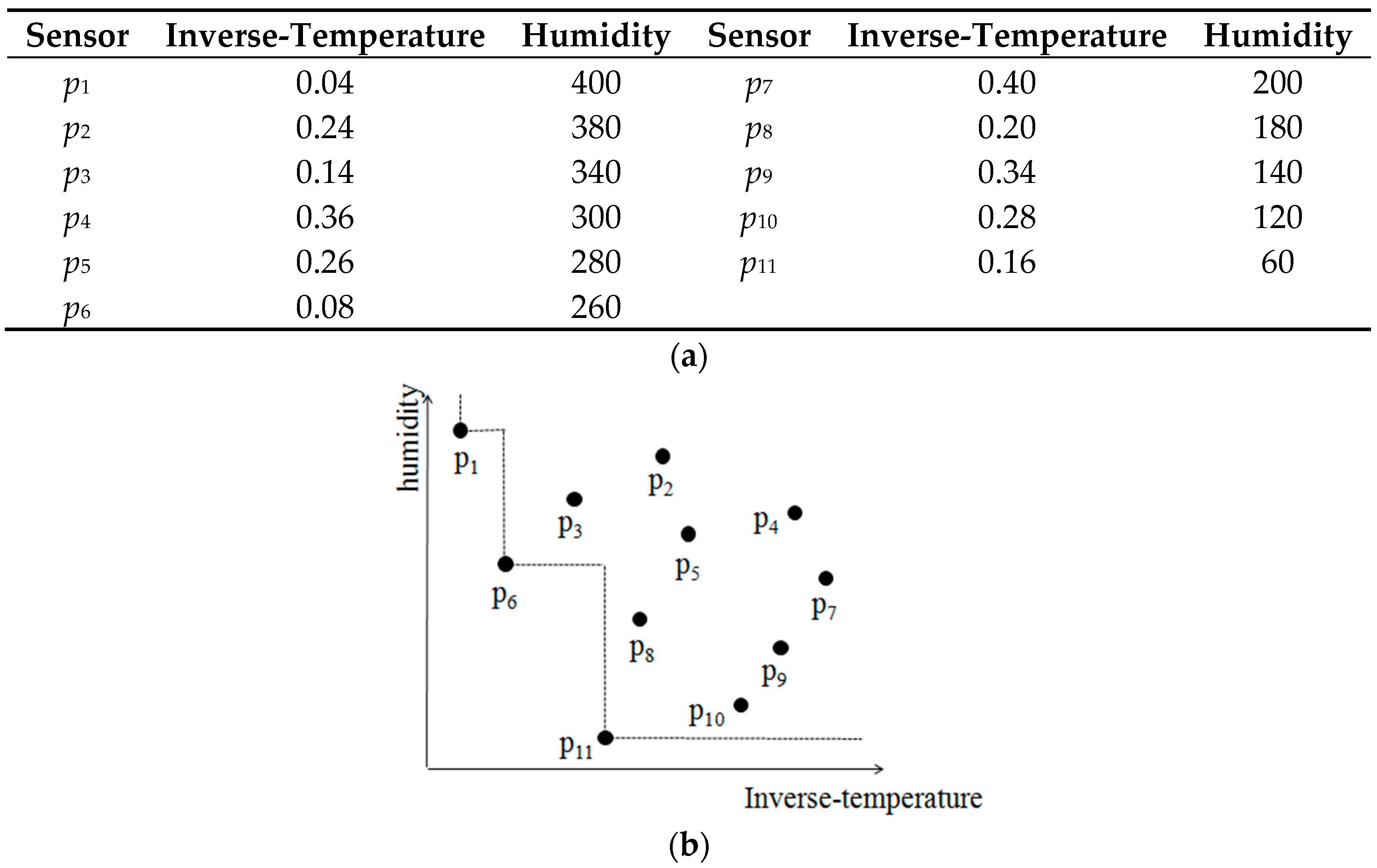
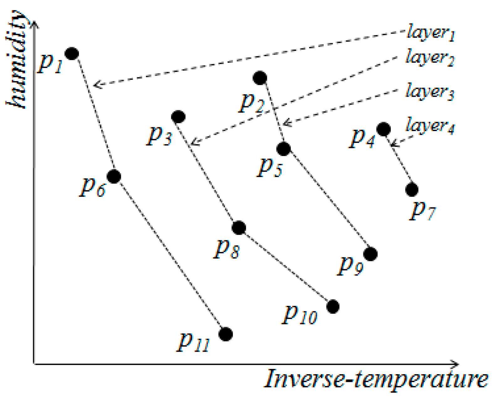
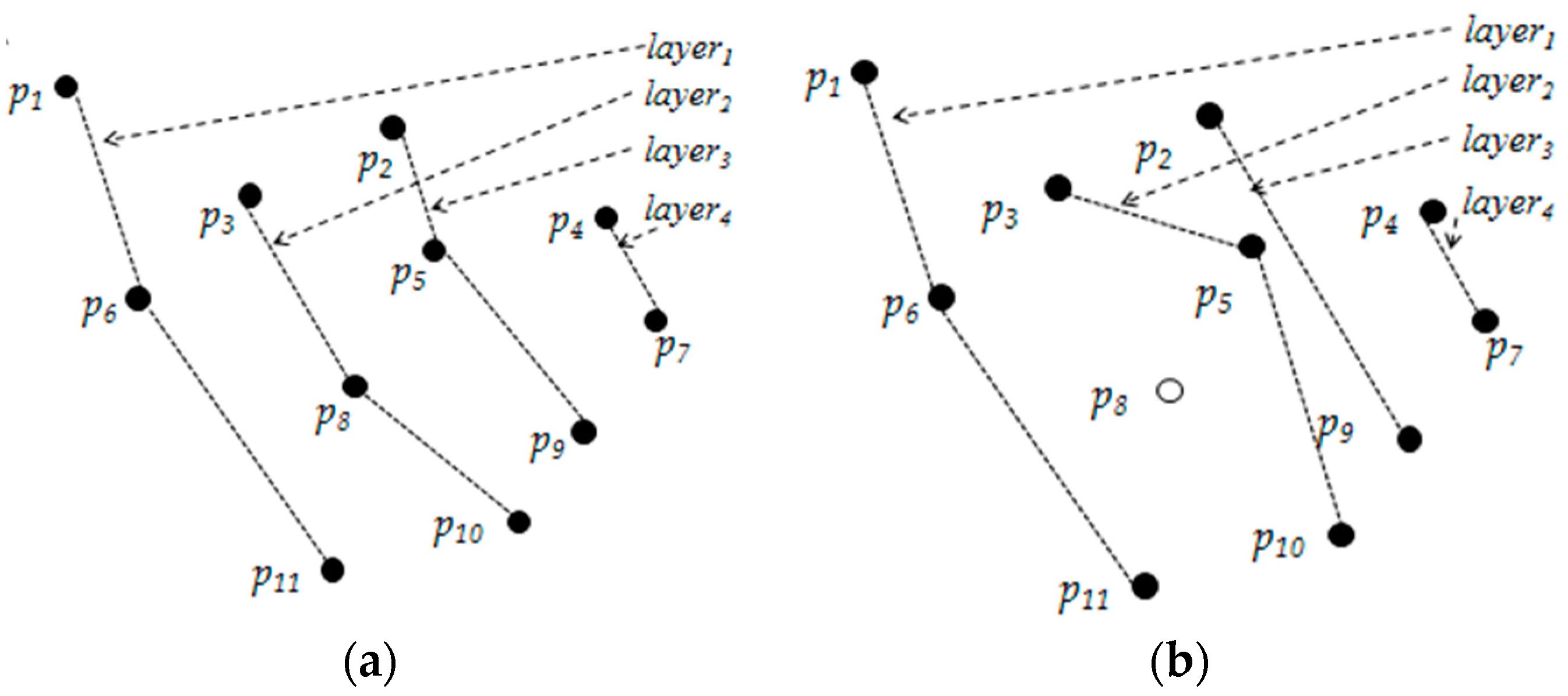
Skyline Layers. Firstly, all the points in D with 2-dimension are sorted with increasing x-coordinate value, then all the points in this order are processed by binary search to find which layer each point belongs to. Because the Pwise algorithm only compute the G-Skyline for the given group size k, so just the first k skyline layers need to be constructed. The point with minimum y-coordinate in layer_i is referred as the tail point of layer_i. An example of skyline layers is shown in Figure 3, and p₁₁ is the tail point of layer₁.

When the dimension space is higher, each point is processed in order and is inserted to a layer or a new layer is started. The data are sorted in one dimension firstly, then in order to find an existing layer the point belongs to, this point should be compared with all points in existing layers.

(2)

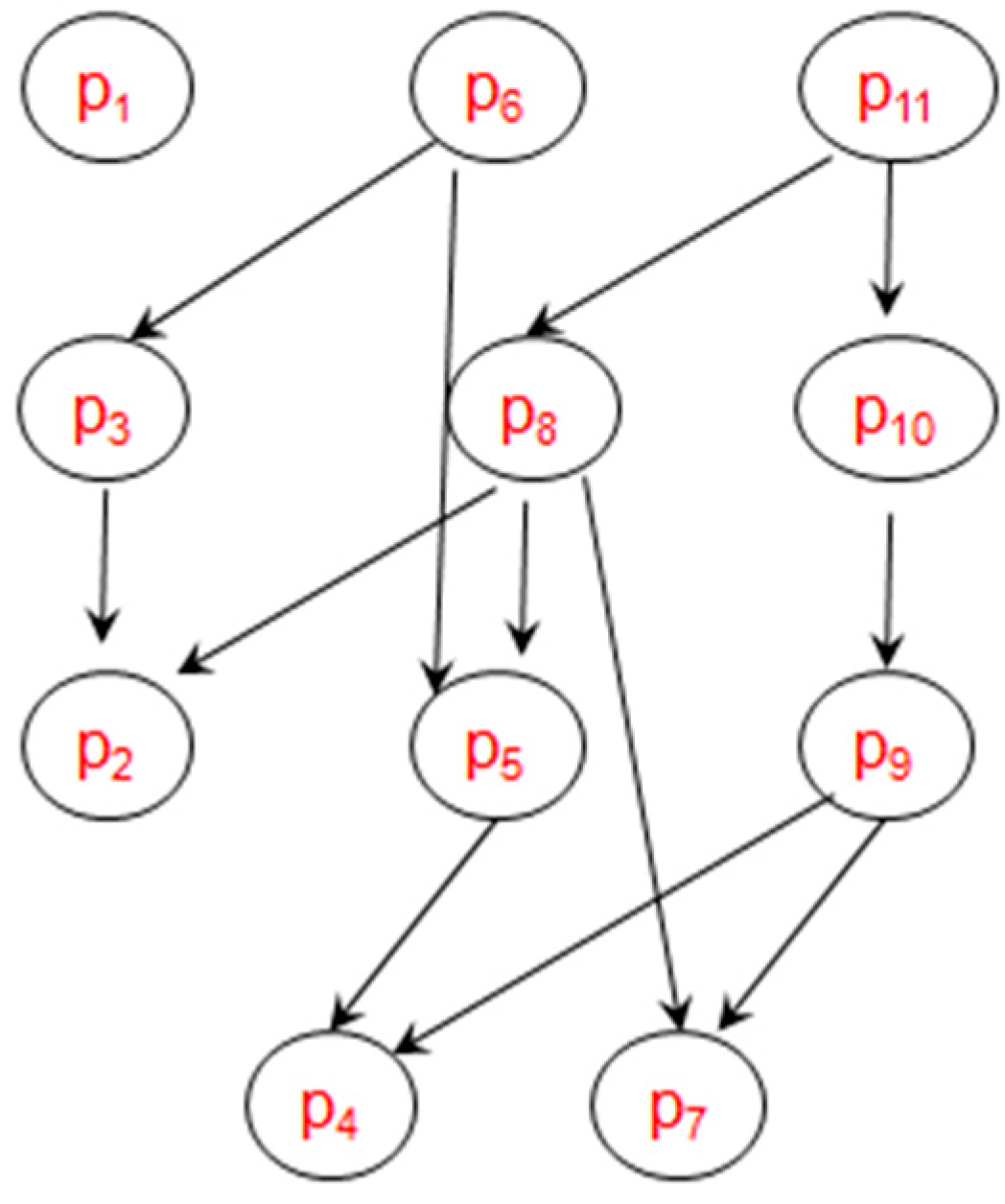
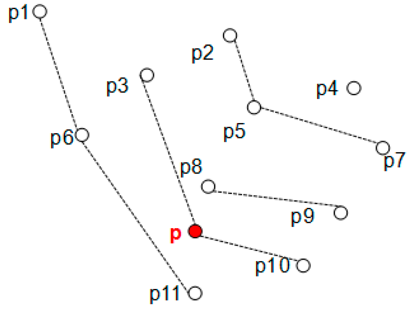
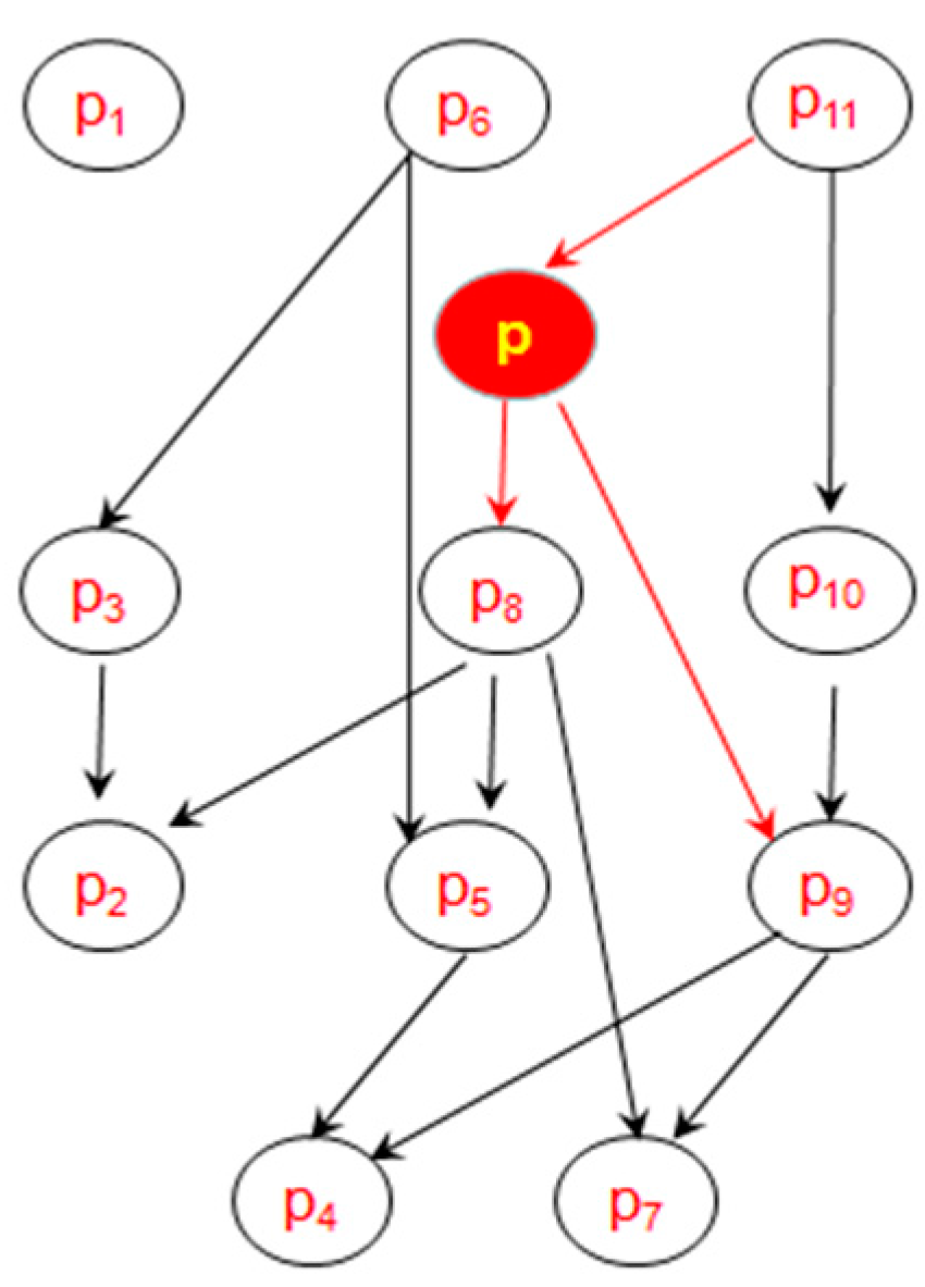
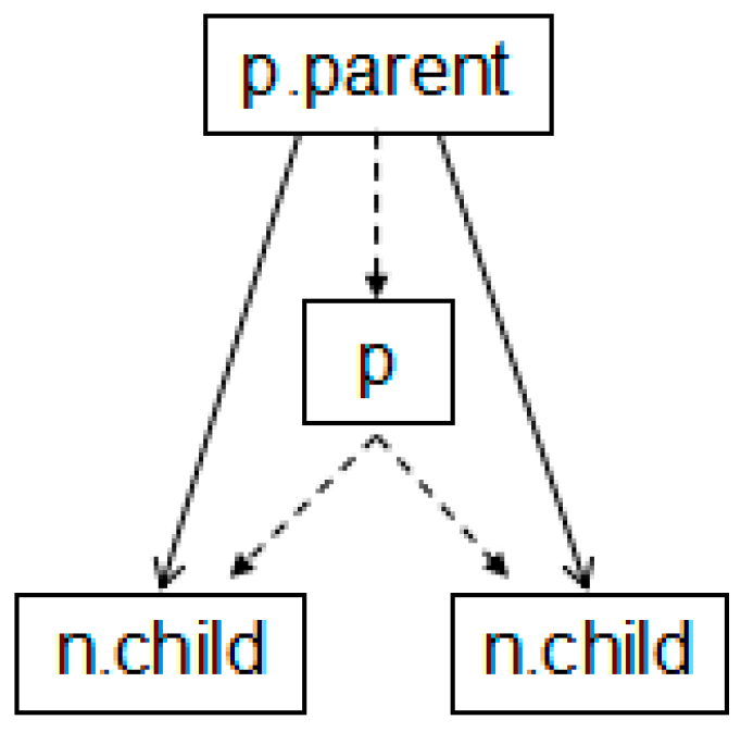
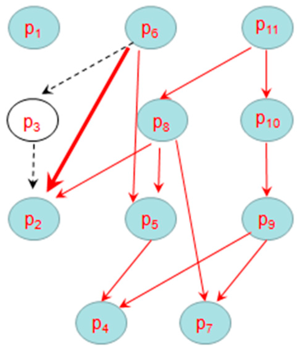
Construct Directed Skyline Graph (DSG). The DSG is a data structure which reflects the dominance relations between the first k layers. It is constructed based on skyline layers: all the points in D are calculated according to the increasing layers. For every point p, it should be compared with all the points in the previous layers and get their dominance relations, for the points which dominate p, they will be added to p’s parents list, and p will be added to their children list. An example of DSG is shown in Figure 4 based on the data in Figure 1. In order to look clarity, all the indirect dominant relations are omitted, such as p₁₁$\prec$ p₂.

(3)

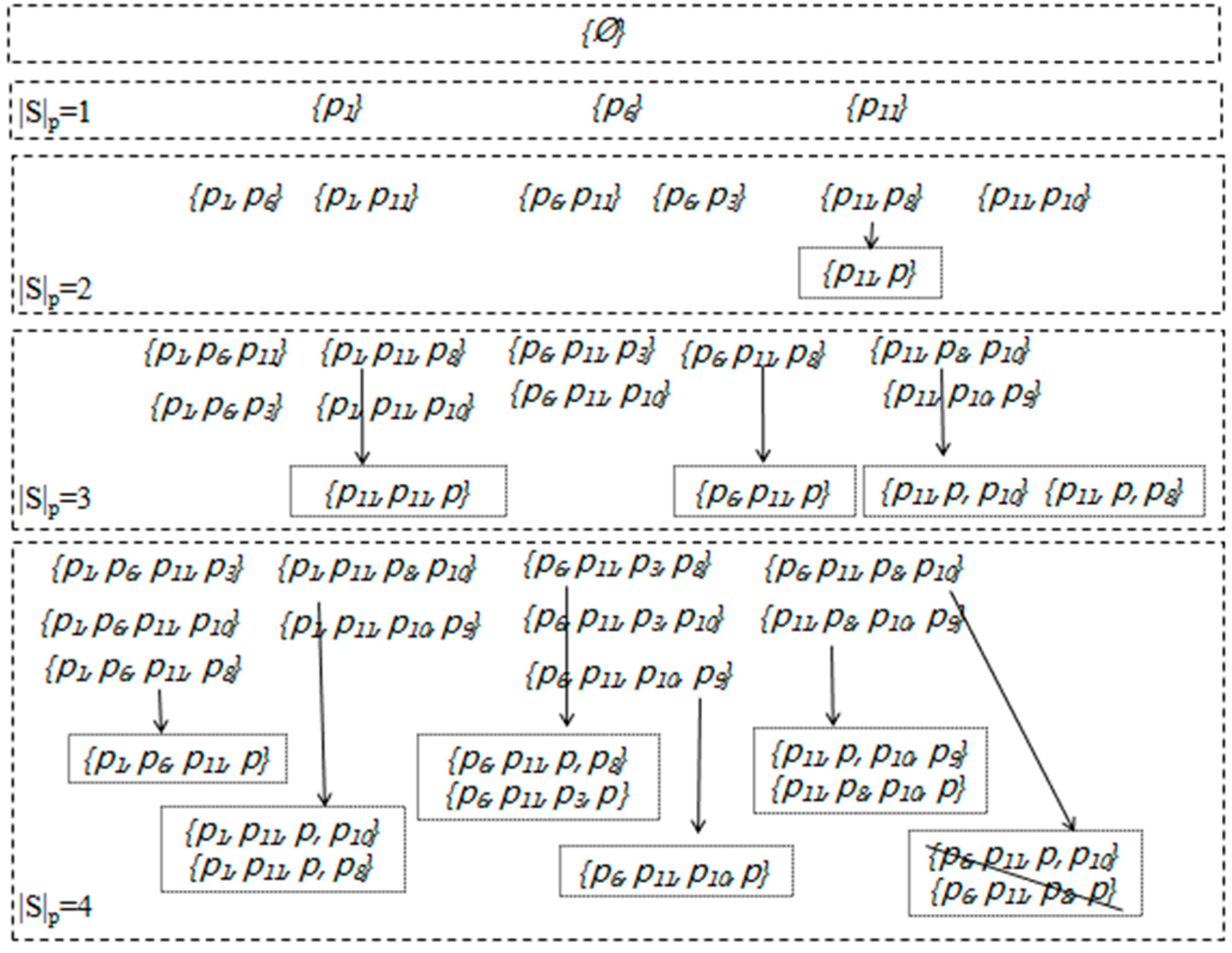
Compute G-Skyline. Based on the skyline layers and DSG, the algorithm performs by the classic set enumeration tree search framework. According to Theorem 2, the algorithm firstly prunes the non-G-Skyline groups as soon as possible, because if a group is not the G-Skyline group, it should not be expanded further, then according to Theorem 3, the algorithm prunes the point from the tail set of each node. Finally, the G-Skyline is returned.

3.3. Our Problem

The points in the static data set are stable, but the points in the data stream are dynamic, each point has its life cycle which is from its arriving time to its expiring time, and the point is only valid during its life cycle. Thus, the active data set of the data stream is not static, and it will change when a new point arrives or an old point expires. Aiming at this problem, we propose an algorithm to find G-Skyline over the data stream. To the best of our knowledge, this problem is the first time to be considered here, and there has been no algorithm can solve it.

In this paper, we use sliding window to manage the data in the stream. There are two type sliding windows (see [34]): the one based on time, and another based on count. We focus on the time-based sliding window.

Definition 5.

(Sliding Window)For a time window W, and t is a random moment, when the point p arrives at t, its life cycle can be written as [t, t + W], and the point is only valid during this period, that is to say the point p is added to the active data set at t moment and is deleted from the active data set at t + W monent.

Theorem 4.

Given a group G with k points coming from the dataset D, for each point p∈G, if all of its parents are in G, or it is the traditional skyline point of D, we can say G is G-Skyline group.

Proof 

Assume a group G = {p₁, p₂, …, p_k}, each point in G and its parents are in G. If there is another group G’ = {q₁, q₂, …, q_k} can g-dominate G, we can find two permutations that for i∈[1,k], q_i $\prec$ p_i, so q_i is p_i’s parent. From the known condition, we conclude that each q_i is in G, G and G’ have the same items. So there is not such a group which g-dominates G, according to the concept of G-Skyline, we can say G is a G-Skyline group. ☐

4. G-Skyline Query over Data Stream

In this section, we elaborate the algorithm to compute G-Skyline in the data stream. For convenience, we maintain that: (1) the layer of point p, denoted by p_l, indicating which skyline layer the point p belongs to; (2) each point has the constant life cycle, denoted as [p.t_arr, p.t_exp], while p.t_arr means when the point p arrives and p.t_exp indicates when the point p expires, p.t_exp = p.t_arr + W.

In order to compute G-Skyline effectively, we present the sharing strategy, and based on which we propose two algorithms to find G-Skyline groups in the data stream.

4.1. Sharing Strategy

Hypothesis 1.

When the point arrives or expires in a data stream, we can update the G-Skyline based on the existing G-Skyline.

Proof of Hypothesis 1.

The dynamic of the data stream reflects in two aspects: new point arriving and old point expiring. Here we take point p as an example. Both cases will result in the active data set changing, and the G-Skyline of active data set will also change. However, not all of the dominance relationships between the points are affected in these two cases, and only such relations are affected: the dominance relationships between p and its parents, and the dominance relationships between p and its children. According to Theorems 1 and 2, we find that when a new point p arrives, the non-G-Skyline groups are still non-G-Skyline groups, and the G-Skyline groups not containing p’s children are still G-Skyline groups, we should only check the other existing G-Skyline groups and the new groups containing p. When an old point p expires, the existing G-Skyline groups not containing p are still G-Skyline groups, and the existing G-Skyline groups containing p should be deleted, so we should check the status of some non-G-Skyline groups.

That is to say, when the active data set changes, we do not have to computing all the active data, we can compute the new G-Skyline based on the existing G-Skyline. ☐

In the G-Skyline processing over the data stream, this sharing strategy will prune most of groups which will not affect the new G-Skyline, and help us to compute the G-Skyline quickly in the data stream.

4.2. Computing G-Skyline for Point Arriving

When a new point p arrives, we should firstly check which layer the point p belongs to, then we update the DSG to construct the new relationships between all the points, finally, we compute the G-Skyline based on the sharing strategy. In order to compute the G-Skyline continuously in the data stream, we should compute the skyline layers and the DSG for all the active points rather than the first k skyline layers and the DSG in the PWise (see [1]).

Update the Skyline Layers for Two Dimensions. For the existing active points, their skyline layers have been constructed, and the points in each layer have been sorted increasingly by x coordinate. When a new point p arrives, by computing p and the tail point of each layer, we can execute the bin-search to find which layer this new point belongs to, then if layer_i.tail does not dominate p and layer_i−1.tail dominates p, we can say p belongs to layer_i. If p is dominated by the tail point of the last layer, it will belong to a new layer. Then we can compare p with all the points in this layer to determine which position the point p locates.

Example 2.

We show an example of Algorithm 1 in Figure 5 based on Figure 1, and we use red circle to indicate the new point. Assume the active points in the data stream are these 11 points, at this moment, a new point p(0.18,130) arrives, so the active data set will change. By updating the skyline layers, we firstly execute the bin-search to find that p locates between layer₁ and layer₂, then we construct the new skyline layers as shown in Figure 4. From the new skyline layers, we find that the layers of some points have changed. For example, p₈ is in layer₂ previously, when p arrives, the point in layer₂ dominated by p is only p₈, so p₈ moves to layer₃, at the same time, as the children of p₈, p₂ and p₅ also move to higher layer₄, similarly, as the child of p₅, p₄ moves to layer₅.

Algorithm 1. Update Skyline Layers When New Point Arrives

Input: the skyline layers of n active points, a new arriving point p

Output: the new skyline layers of active points

1 for I = 1 to maxlayer do

2 if the layer1’s tail point does not dominate p then

3 p.layer = 1;

4 else if layermax’s tail point dominates p then

5 p.layer = maxlayer + 1;

6 else

7 calculate bin-search to find which layer p belongs to

8 compare p with the points in p.layer to determine p’s position in the layer

9 if there is a point in p.layer is dominated by p

10 Denote all the points in p.layer dominated by p as D1

11 While (D1! = null)

12 {For each point q in D1

13 Copy all the points in layer(q.layer+1) dominated by q to D2

14 q.layer = q.layer + 1;

15 delete q from D1;

16 D1 = D2;

}

17 return the new skyline layers

Update the Skyline Layers for Higher Dimensional Space. When the dimension of dataset is higher, an algorithm similar to Algorithm 1 can be used to update the layers. Firstly, we copy the dataset to d copies, then each copy is sorted by a different coordinate in ascending order, this work is a foundation and should be just done once. Secondly, when a new point p arrives, we can perform a bisearch to find where p locates in each copy and insert it to that copy, then if a point locates bebind p in all copies, this point must be dominated by p. We can easily get the minimum layer of all the points dominated by p, and we set this layer as layer_m, then this new point p either belongs to layer_m or layer_m−1. If p is dominated by a point in layer_m−1, then p belongs to layer_m, and each point dominated by p will move to higher layer. Otherwise if p is not dominated by a point in layer_m−1, p belongs to layer_m−1, and each point dominated by p still stay its current layer.

Update the Directed Skyline Graph (DSG). When the new point p arrives, it changes the skyline layers, because the DSG is built based on the skyline layers, so we should also update the DSG of the active points.

According to the DSG concept, we know that when a new point p arrives, it does not affect other points except for its parents and children. So the DSG updating can be finished in two steps. Firstly, to find p’s parents, we can compare p with each point whose layer is smaller than p’s layer, if a point q is p’s parent, we should not compare p with q’s parents. Secondly, to find all of p’s children, we can compare p with each point whose layer is larger than p’s layer, if a point q is p’s child, we should not compare p with q’s children. This method is also suitable for higher dimensional space.

Example 3.

We show an example of DSG updating in Figure 6 based on Figure 1, and we use the red circle to indicate the new point. When a new point p(0.18,130) arrives, we firstly update the skyline layers, then we can update the DSG to reflect the dominance relationships in real time. Because p lies between layer₁ and layer₂ in the old skyline layers, we can find p is dominated by p₁₁ in the layer₁, p₈ in the layer₂ is dominated by p, and p₈ is the child of p₁₁ previously, so we set p₁₁ as p’s parent, and p₈ as p’s child, then the children (p₂, p₅, p₄, p₇) of p₈ will not be compared with p, and we also find p₉ is also p’s child. The new DSG is shown in Figure 6. We can see that when a new point p arrives, there are some dominant relationships about p added to DSG, but other dominance relationships irrelevant to p will remain unchanged.

Compute G-Skyline for a point arriving. After updating the skyline layers and DSG, we can compute the new G-Skyline based on the existing G-Skyline. According to Theorem 1, we infer that which layer p belongs to will generate different effect on the new G-Skyline. So we present different solutions on the basis of p’s location as follows.

Hypothesis 2.

(1) 

If p._layer > k. According to Theorem 1, the point of G-Skyline groups must in the first k layers, so if p._layer > k, pwill not affect the G-Skyline result.

(2) 

If p_.layer < k. In this case, p has no effect on the non-G-Skyline groups and the G-Skyline groups which do not contain all of p’s parents. However, the point p may only affect the G-Skyline groups which containing all of p’s parents, here we denote these groups as candidate groups.

Proof of Hypothesis 2.

For the non-G-Skyline groups G₁, there must be a group G₂ dominating it, when p arrives, G₂ still dominates G₁, so we can easily find p has no effect on such kind of groups.

For each G-Skyline group G₃ not containing all of p’s parents, according to Theorem 3, there must be no child of p existing in G₃, so there is no point dominated by p, and p has no effect on the G-Skyline groups not containing all of p’s parents.

For the G-Skyline groups not containing any parent of p, we can easily prove p has no effect on such kind of groups. Finally, only the G-Skyline groups containing all of p’s parents should be re-evaluated. ☐

We call this kind of groups the candidate groups, and we divide the candidate groups into two kinds, and give different solutions for them. If there is not any G-Skyline group containing all of p’s parents, p will not affect the query result.

Solution 1.

For each G-Skyline group G which contains all parents of p except for p’s children, p will not affect its status. We can replace the leaf point of G by p to compose the new group which is G-Skyline group, while this leaf point cannot be p’s parent. However, G is still G-Skyline group.

Proof of Solution 1.

Assume G is a G-Skyline group not containing p’s children, that is to say, there is not any point in G dominated by p, and there will be no group containing p can dominate G, so p does not affect G’s status, and G is still G-Skyline group. On the other hand, if we replace the leaf point of G by p to compose the new group G’, we cannot find another group which can dominate G’ because all of p’s parents are already in G, so G’ is G-Skyline group too. ☐

Solution 2.

For each G-Skyline group containing p’s children, p will affect the its status. We replace the leaf point of G by p to compose the new group which will be G-Skyline group. However, G is not G-Skyline group yet.

Proof of Solution 2.

If the G-Skyline group contains p’s children, such as G = {g₁, g₂, …, g_i, …, g_k} and g_i is p’s child, we can find G’ = {g₁, g₂, …, p, …, g_k} can g-Dominates G because p $\prec$ g_i, so the group G will not be G-Skyline. At the same time, if we replace the leaf point of G by p to compose a new group G’, then each of the point in G’ and all of its parents are in the G, so according to concept of G-Skyline and Theorem 4, we can see that there is no group which can g-Dominate G’, so G’ is G-Skyline group. ☐

According tothe above solutions, when a new point arrives we can quickly find the new G-Skyline based on the existing G-Skyline groups. The process is shown in Algorithm 2 as follows.

Algorithm 2. Point-Arriving-Algorithm

Input: a data set D with n active points, the corresponding skyline layers and DSG, group size k, a new arriving point p

Output: New G-Skyline groups

1 update the skyline layers

2 update the DSG

3 for each group G in G-Skyline

4 if G contains all of p’s parents

5 if G does not contain p’s child

6 G’ ← replace the leaf point of G by p

7 insert G’ to G-Skyline

8 if G contain p’s child

9 G’← replace the leaf point of G by p

10 insert G’to G-Skyline

11 remove G from G-Skyline

12 return New G-Skyline

Example 4.

An example of Algorithm 2 is shown in Figure 7 based onFigure 1. Assume at present the active points in the data stream are these 11 points. The k-item G-Skyline groups are shown in Figure 7 where 1 ≤ k ≤ 4. When a new point p(18,30) arrives, after updating the skyline layers and DSG, we can begin to update the relevant groups. The parent of p is only p₁₁, so each G-Skyline group containing p₁₁ should be expanded. For visualization clarity, we omit the reduplicate new G-Skyline groups coming from the existing G-Skyline groups. The groups in the dotted box are new groups born from the existing G-Skyline groups. At level |S|_p = 1, we can easily find that p’s arriving has no effect on the 1-item G-Skyline. At level |S|_p = 2, among the existing 2-item G-Skyline groups, we find the group {p₁₁, p₈} contains the parent and the child of p, according to solution 2, we should replace p₈ by p to form the new G-Skyline group {p₁₁, p}, and this new group is G-Skyline group, but the group {p₁₁, p₈} will be no longer the G-Skyline group because it is g-dominated by the new group {p₁₁, p} . Similarly, for the group {p₆, p₁₁, p₈}, it also contains the parent and the child of p, so we get the new G-Skyline group {p₆, p₁₁, p} instead of {p₆, p₁₁, p₈}. As a result, level |S|_p = 4 shows all the 4-item G-Skyline groups without checking.

Obviously, the above algorithms are used to compute the G-Skyline whenever a new point arrives. However, if there is a group of points which arrives at the same time, we can also use these algorithms similarly. Firstly we should use Algorithm 1 to update the skyline layers by processing these points one by one, then we update the DSG in the same way, and finally we compute the G-Skyline by Algorithm 2 for each new arriving point. However, this direct solution is only suitable for a little group of points arriving at the same time, when the group is large, this solution is useless and this is what will be considered in our future work.

4.3. Updating G-Skyline for Point Expiring

Each point in the data stream has its life cycle, when an active point expires, the active data set will change too, so we should compute the new G-Skyline groups of the new active dataset based on the existing result. In this section, we firstly update the skyline layers, then reconstruct the DSG, finally compute the G-Skyline for point expiring.

Update the Skyline Layers for Two Dimensions. Different form the point arriving, when a point expires, we can easily update the skyline layers. Assume point p in layer_L expires, if p is the tail point of layer_L, each tail point of layer_L’ (L’ > L) will be moved to the tail of layer_L’−1, at the same time, any other points still locate in their previous layer. If p is not the tail point of layer_L, we will not only delete p, but also change the layers of some points. If point q is in layer_L+1 and its parent in layer_L is just p, then we can move q to layer_L. Then we will similarly change the layers of some points one layer by one layer. The procedure of updating skyline layers is shown in Algorithm 3.

Algorithm 3. Update Skyline Layers for Point Expiring

Input: the skyline layers of n active points, a point p to expire

Output: the skyline layers of active points

1 if p is the tail point of layerL

2 for I = L to maxlayer-1 do

3 (layeri).tail = (layeri+1).tail;

4 else

5 Initialize a set S = null;

6 L’ = L;

7 copy p to S;

8 while(S! = null)

9 {for each point p’ in S

10 {for each child q in layerL’+1 of p’

11 {if S contains all parents of q in layerL’

12 q.layer = q.layer− 1;

13 copy q to S;

}

14 L’++;

15 delete p’from S;

}

}

16delete p

17return the new skyline layers

Example 5.

An example of Algorithm 3 is shown in Figure 8 based on Figure 1. For the 11 active points, if the tail point expires, we should firstly delete this tail point, then change the tail point of layer_i+1 to the tail point of layer_i, other points keep their layers unchanged. As shown in Figure 8a, when the tail point p₁₀ expires, p₉ becomes the tail of layer₂, and p₇ becomes the tail of layer₃, where in the previous layers p₉ was the tail of layer₃ and p₇ was the tail of layer₄. However, when point p₈ expires, we find p₈ is p₅’s single parent in layer₂, so we move p₅ to lower layer₂, but p₄ still lie in its original layer because the parents of p₄ in layer₃ are p₅ and p₉ while only p₅ is in S, the new skyline layers is shown in Figure 8b.

Update the Skyline Layers for Higher Dimensional Space. When the dimension of dataset is higher, an algorithm similar to Algorithm 3 can be used to update the layers. When point p in layer_L expires, for each child q of point p in layer_L+1, if p is its single parent in layer_L, then p will move to layer_L, otherwise p will stay its layer as it is dominated by other points in layer_L. Recuirsively, we check all the children of the point whose layer changes in the same way.

Update the Directed Skyline Graph (DSG). When an old point expires, it maybe affects the existing skyline layers, and it maybe also changes the DSG.

The DSG reflect the dominance relationships of each point, so when point p expires and is removed, there will be no relationships between it and its parents, and between it and its children. In the DSG, the directed edge indicates the dominance relationship, so when p expires, the edges between p and its parents and the edges between p and its children should be deleted, at the same time, the new directed edges from p’s parents to p’s children will be added to DSG, the procedure is shown in Figure 9. In fact, the dominant relationships indicated by new directed edges have been existed already, just because we omit them for visualization clarity. The most importance is p’s expiration will not change the dominance relationships between other points.

Example 6.

We give an example to show the DSG updating when an old point expires in Figure 10 based on Figure 1. Assume there are 11 points in data stream, when the expiration time of p₃ arrives, the point p₃ will be deleted. Then the dominance relationships about p₃ will be removed from DSG, at the same time, the new directed edges between its parents (such as p₆) and its children (such as p₂) will be added to DSG.

Compute G-Skyline for a point expiring. Similar to the G-Skyline computing for point arriving, after updating the skyline layers and the DSG, we can compute the new G-Skyline groups based on the existing G-Skyline. According to the G-dominate concept and Theorem 3, we find that the expiration of point p only has an effect on the G-Skyline groups which contain p or p’s children, it will not affect any other groups. Next, we analyze whether these groups are new G-Skyline groups or not.

(1) For the G-Skyline groups

If G is a G-Skyline group and does not contain p, according to G-Skyline concept, there is not a groups G’can G-dominate G, we can easily know that p’s expiration does not affect such groups.

If G is a G-Skyline groups and contains p, we can get the new k-item G-Skyline group by deleting p from the old k+1-point G-Skyline groups.

Proof of (1).

From the algorithm for the static data set, we know that the G-Skyline groups with k+1 points come from G-Skyline with k points. Assume that G = {q₁, q₂, …, q_k, p } is G-Skyline groups with k + 1 points, and it maybe contains p’s children, we know that each point in G and all of its parents are in G. When p expires and is deleted from G, G’ = G−p = {q₁, q₂, …, q_k}, and each point in G’ and all of its parents are still in G’, according to Theorem 4, we can say G’ is G-Skyline groups with k points when p expires. ☐

(2) For the non-G-Skyline groups

If G is a non-G-Skyline group and contains p, it can be deleted safely.

If G is a non-G-Skyline group and does not contain p, it maybe becomes G-Skyline group when p expires.

Proof of (2).

We can easily prove the conclusion when G is a non-G-Skyline group and contains p when p expires. However, when point p expires, it will not dominate its children anymore, so some of non-G-Skyline groups which does not contain p but contains p’s children maybe becomes G-Skyline. According to Theorem 4, these groups must satisfy the condition: for such group G, each of point in G and all of its parents except p must be in G. Because p’s children’s parents contain p’s parents, so if we add p to G to form G’ with k + 1 points, G’ must be k + 1-point G-Skyline group of the active data set before p expires. Then we can get these candidate groups by deleting p from the k + 1-item G-Skyline groups, and these groups have been returned in (1). However, any other non-G-Skyline groups which do not meet this condition will not belong to G-Skyline, and they can be pruned safely. ☐

When a point p expires, we can quickly compute the new G-Skyline groups based on the existing G-Skyline groups. Based on the above strategy, our key idea of the algorithm is shown in Algorithm 4.

Algorithm 4. Point-Expiring-Algorithm

Input: a data set D with n active points, the corresponding skyline layers and DSG, group size k, a point p to expire.

Output: New G-Skyline groups NGS

1 update the skyline layers

2 update the DSG

3 for each group Gk in G-Skyline

4 if G does not contain p

5 Copy Gk to NGS

6 for each group Gk+1 containing p in G-Skyline

7 G’ ← remove p from Gk+1

8 insert G’ to NGS

9 return NGS

Example 7.

Now we show an example of Algorithm 4 in Figure 11 based on the data in Figure 1. Assume the active points of data stream at present time are these 11 points. When an old point p₆ expires, p₆ will be useless, and the active points data set will change, so we should compute the new G-Skyline. At level |S_p|=1, we firstly delete p₆, then get the new 1-point G-Skyline group p₃ by removing p₆ from {p₆, p₃} which is 2-point old G-Skyline group, and we set a dashed box to denote the new G-Skyline group. At the same level, we can also remove p₆ from {p₁, p₆} and {p₆, p₁₁} to get the new skyline point p₁ and p₁₁, but these two points already belong to skyline, for visualization clarity, we do not show this kind of indications. Similarly, at the level |S_p|=2, we can get the new 2-point G-Skyline groups {p₁, p₃} and {p₁₁, p₃} by removing p₆ from the old 3-point G-Skyline groups {p₁, p₆, p₃} and {p₆, p₁₁, p₃}. As a result, level |S_p|=3 shows all the new G-Skyline groups with 3 points. Based on our pruning strategies, we can easily get the new G-Skyline groups at each level without much computation.

Similarly, if there is a group of points which expires at the same time, we can take the similar approach as the one which is used to process points arriving at the same time: update the skyline layers by Algorithm 3 to process these points one by one, then update the DSG, finally compute the G-Skyline by Algorithm 4 for each point which expires. This solution is only suitable for a little group of points expiring at the same time, and we will consider how to process a big group of points expiring at the same time in our future work.

5. Experiments

In this section, we present experimental evaluation about our algorithms. In order to avoid the limitations of data from a particular domain to the experiment results, we select the synthetic data.

5.1. Experiment Preparation

We simulate a data stream and evaluate the algorithms when the new data arrives or the old data expires. For each condition, we firstly evaluate the skyline layers updating, and then perform the comprehensive experiments to test the G-Skyline algorithm based on the synthetic data. To examine the extendibility of our algorithms, we generate three critical types of data: the correlated data (COR), the independent data (IND) and the anti-correlated data (ANTI-COR). The example of each type of data with 200 points with 2-dimension is shown in Figure 12, we can find that their distributions are different from each other: the two coordinates of the correlated points have the same variation trend, and this kind of points which are good in one dimension are also good in other dimension; while the two coordinates of the anti-correlated points have the opposite variation trend, and this kind of points which are good in one dimension are bad in other dimension; however, the two coordinates of the independent points have no relation in the variation trend. For the correlated dataset and the anti-correlated dataset, the points are generated by selecting a plane perpendicular to the line from (0, …, 0) to (1, …, 1) using a normal distribution, while for the independent dataset, all attribute values of points are generated independently using a uniform distribution.

Because this is the first time to compute G-Skyline over the data stream, our examine evaluation was conducted against the existing algorithm for static dataset. All the experiments are performed on a PC with 1.7 GHz Intel Core i7 processor running Windows 7 operation system with 8GB memory and 1TB hard drive. The algorithms to be examined in the experiments are as follows.

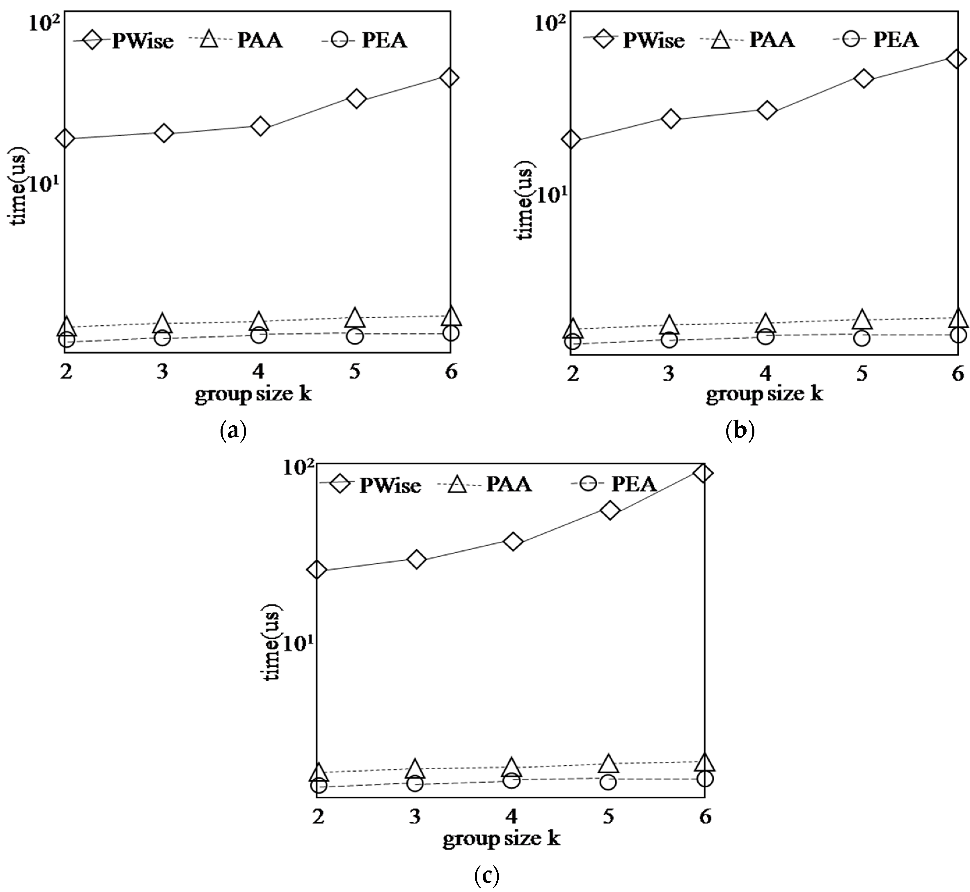
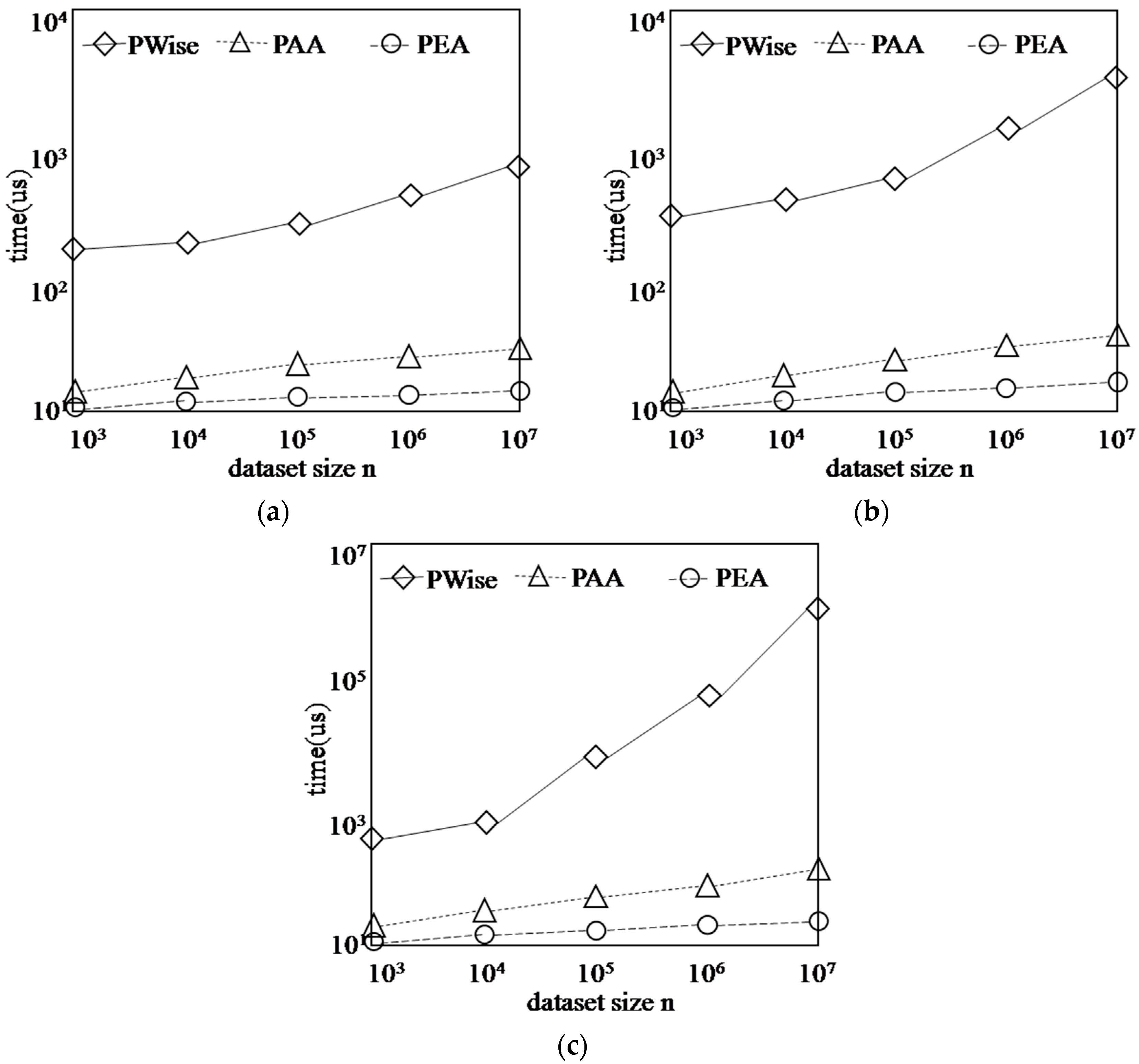
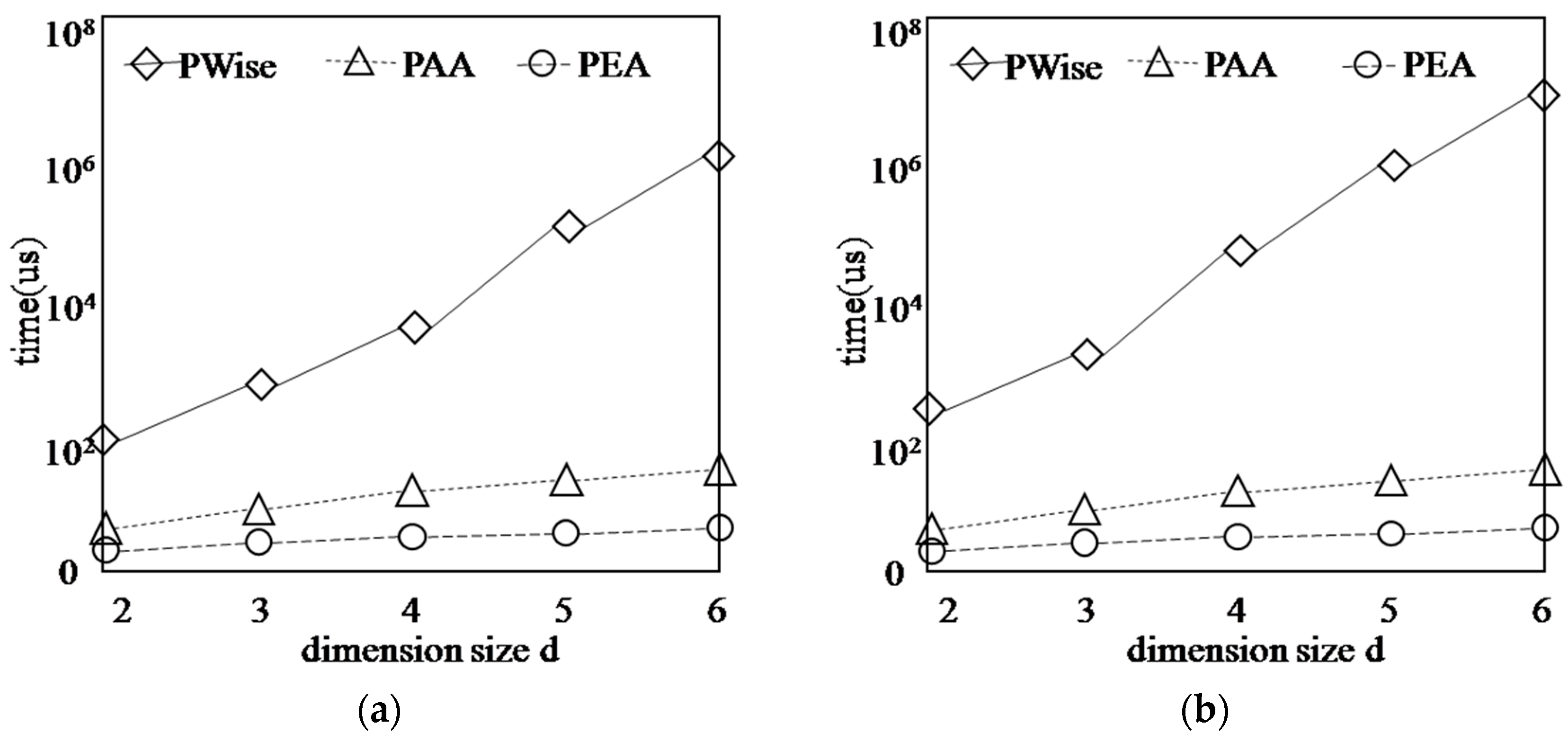
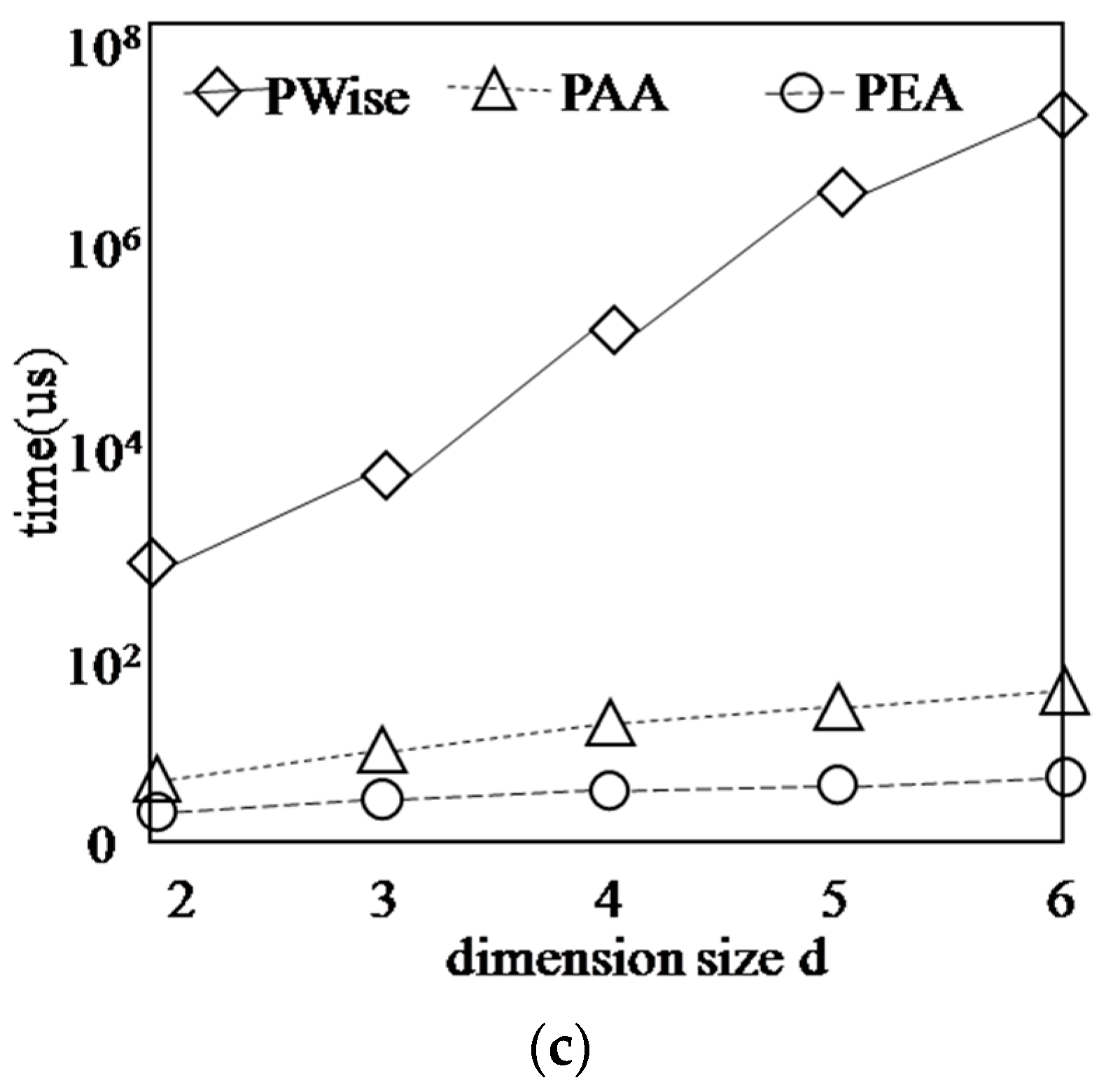
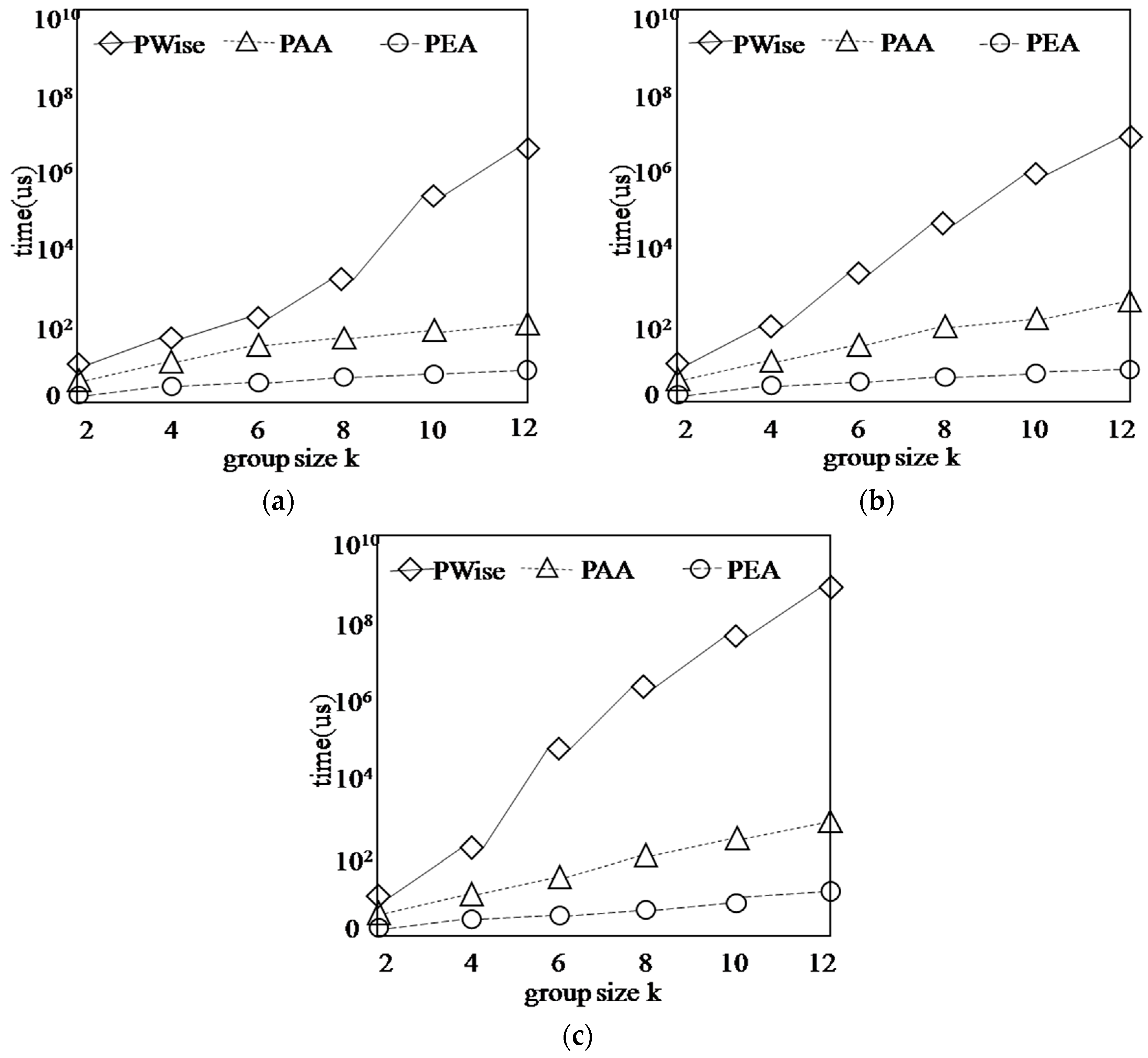
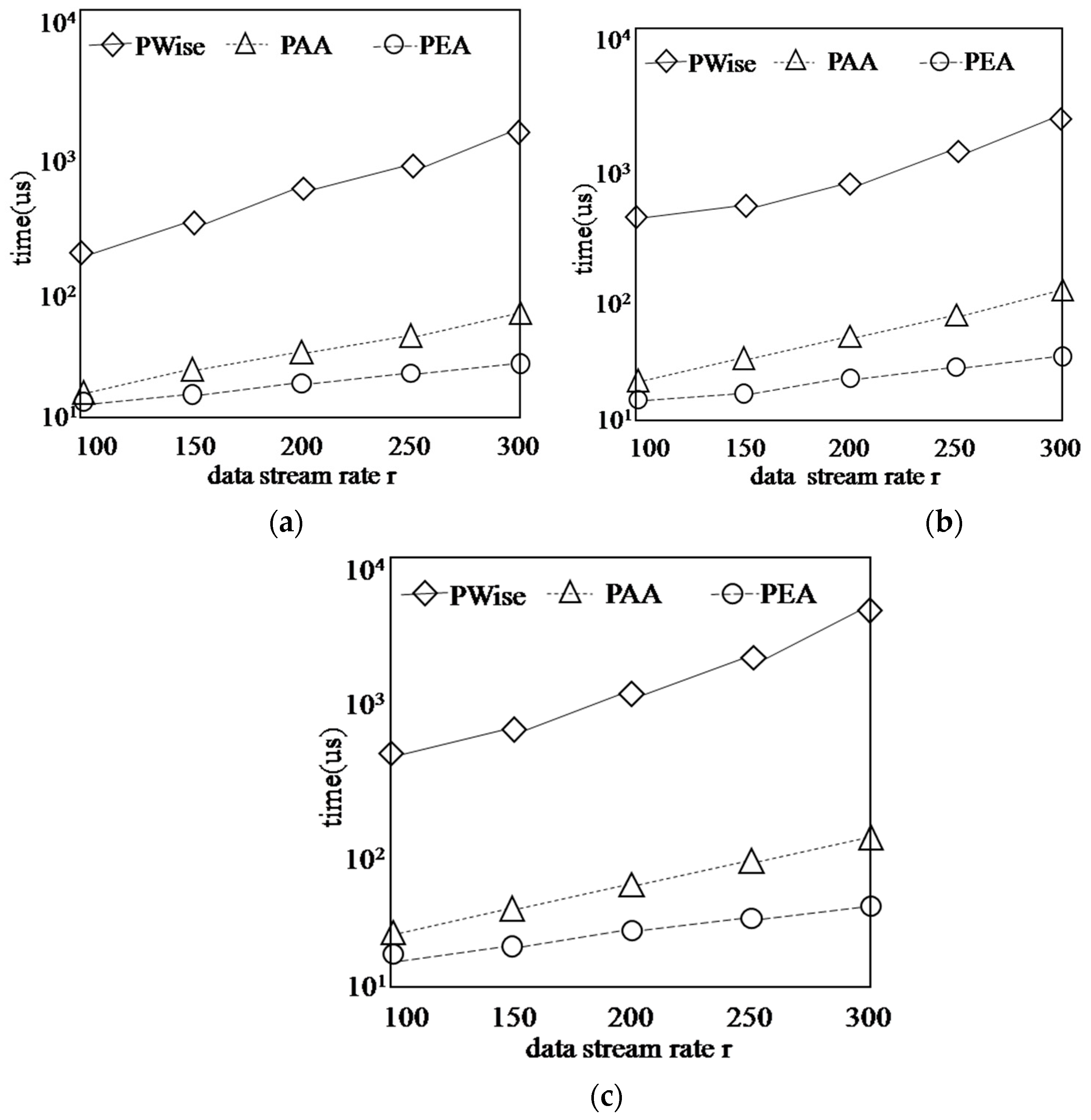
• PAA: Computing G-Skyline groups for a new point arriving.
• PEA: Computing G-Skyline groups for an old point expiring.
• PWise: Point-Wise algorithm of G-Skyline for static dataset in paper [1].

5.2. Updating Skyline Layers

Firstly we examine our algorithms for updating skyline layers when the new point arrives or an old point expires. The PWise algorithm is to rebuild all the skyline layers by binary searching for the new active dataset, while our algorithm can update the skyline layers directly based on the existing skyline layers. Here the running time of PWise refers to the average time which is taken to update skyline layers for a point arriving and a point expiring, the running time of PAA refers to the time which is taken to update skyline layers for a point arriving, and the running time of PEA refers to the time which is taken to update skyline layers for a point expiring. The experiments are repeated 100 times and the average value is used as the final result.

Figure 13 shows the running time cost of updating skyline layers in the PWise algorithm and our algorithms on the different datasets. When the group size k varies from 2 to 6, we find that the PWise algorithm is affected by the different datasets and the growth of running time is flat from correlated dataset to independent dataset, and to anti-correlated dataset. The reason is that the PWise algorithm only considers the points in the first k skyline layers while other points will not be considered. Different from PWise, our algorithms perform better. The reason is that when a new point p arrives in the data stream, based on the existing skyline layers, we should only use binary search to find where p will locate. In order to compute the G-Skyline continuously, the skyline layers in our algorithm must contain all of the active points, so no matter what value the group size k is, for the same dataset, the running time of updating skyline layer is same, and it is much less than PWise. However, when an old point p expires, to update the skyline layers, our PEA can directly delete the p and change the layers of some points dominated by p. This work is more easy and the running time is the most least.

According to the distribution of each dataset, we find that the average layer number follows COR.ln > IND.ln > ANTI-COR.ln. Then the running time of our algorithm shows little growth. Finally, our algorithms perform better than PWise.

5.3. Performance with Respect to the Synthetic Data

In this section, we show the experimental evaluation of algorithms on the synthetic dataset. Each dataset is generated following the seminal work in paper [2]. When the dataset size is more than 10³, adding a new point to the active dataset or deleting an old point from the active dataset has no effect on the total number of points to be computed in PWise, so the running time of PWise for this two cases approximatelyequal, so the running time of PWise refers to the average of total time which is taken to update skyline layers and computing G-Skyline for a point arriving and a point expiring, while the running time of PAA refers to the total time for a point arriving, and the running time of PEA refers to the total time for a point expiring. The experiments are repeated 100 times and the average value is used as the final result.

Figure 14 shows the running time of algorithms on each synthetic dataset with different dataset size n, while d = 2, k = 4. The varying n has a certain effect on the PWise algorithm because it should compute the points in the first k layer, and the total number increases with n increasing, then the running time shows little growth on the COR dataset and IND dataset, while PWise need much time in ANTI-COR dataset because every layer has more points than other two dataset. However, our algorithm perform better. When a new point arrives in the data stream, based on the existing G-Skyline groups, PAA only need to check the groups expanded from the existing G-Skyline groups which contain all of p’s parents, the number of these candidates will not be large, so the running time of PAA is less than PWise. Similarly, when an old point p expires, PEA only needs to check the existing G-Skyline groups which contain p, this is very easy and the running time is very little.

Figure 15 shows the running time of algorithms on each synthetic dataset with different dimension size d, while n = 1000, k = 3. The varying d has much effect on the PWise algorithm because the total number of the points in the first k layers increases sharply with d increasing. However, the running time of our algorithms is less and increase smoothly. The reason is that our algorithms can get the new G-Skyline based on the existing G-Skyline, although the number of points in the first k layers increases sharply, the number of candidates to be checked keeps little growth.

Figure 16 shows the running time of algorithms on synthetic dataset with different group size k, while n = 1000, d = 2. The running time of PWise increases sharply with k increasing, the reason is that the number of points in the first k layers increases quickly. PAA needs a little more time than PEA, this is due to their different solution approach, PAA needs to check more candidates than PEA.

Figure 17 shows the running time of algorithms on synthetic dataset with different data stream rate r, while k = 3, d = 2 and the span of sliding window is 10 s. There are five rates used in the experiments: 100 points per second, 150 points per second, 200 points per second, 250 points per second and 300 points per second. Figure 17 shows that, when the data stream rate increases, the running time of algorithms increase obviously for each type of dataset. The reason is that with data stream rate increasing, the total number of points arriving or expiring within the sliding window must become bigger, and then much more time will be needed for computing.

6. Conclusions and Future Work

Processingdata streams from the sensor network will provide important information for users. In this paper, we proposed the problem of finding G-Skyline groups in the data stream. In order to compute the G-Skyline groups efficiently, we first presented the sharing strategy, and based onthis, we proposed two algorithms PAA and PEA to compute the new G-Skyline groups when a new point arrive or an old point expires. The experiment results based on the synthetic data show our algorithms’ benefit. In the future, we will consider how to compute the G-Skyline groups if a large group of points which arrives or expires at the same time, and querying the G-Skyline groups over the uncertain data stream in the sensor network will be also one of our future research work.

References

1. Liu, J.; Xiong, L.; Pei, J. Finding Pareto Optimal Groups: Group-based Skyline. In Proceedings of the International Conference on Very Large Databases (VLDB), Hilton Waikoloa, HI, USA, 31 August–4 September 2015; pp. 2086–2097. [Google Scholar]
2. Borzsonyi, S.; Kossmann, D.; Stocker, K. The skyline operator. In Proceedings of the 17th International Conference on Data Engineering, Heidelberg, Germany, 2–6 April 2001; pp. 421–430. [Google Scholar]
3. Chomicki, J.; Godfrey, P.; Gryz, J. Skyline with presorting. In Proceedings of the 19th International Conference on Data Engineering, Bangalore, India, 5–8 March 2003; pp. 717–719. [Google Scholar]
4. Tan, K.; Eng, P.; Ooi, B. Efficient progressive skyline computation. In Proceedings of the 27th International Conference on Very Large Data Bases (VLDB), Roma, Italy, 14–15 September 2001; pp. 301–310. [Google Scholar]
5. Kossmann, D.; Ramsak, F.; Rost, S. Shooting stars in the sky an online algorithm for skyline queries. In Proceedings of the 28th International Conference on Very Large Data Bases (VLDB), Hong Kong, China, 20–23 August 2002; pp. 275–286. [Google Scholar]
6. Pei, J.; Jin, W.; Ester, M.; Tao, Y. Catching the best views of skyline: Asemantic approach based on decisive subspaces. In Proceedings of the 31st International Conference on Very Large Data Bases, Trondheim, Norway, 30 August–2 September 2005; pp. 253–264. [Google Scholar]
7. Lee, J.; Hwang, S.W. Toward efficient multidimensional subspace skyline computation. VLDB J. 2014, 23, 129–145. [Google Scholar] [CrossRef]
8. Xia, T.; Zhang, D. Refreshing the sky: The compressed skycube withefficient support for frequent updates. In Proceedings of the International Conference on Management of Data and Symposium on Principles Database and System, Chicago, IL, USA, 27–29 June 2006; pp. 491–502. [Google Scholar]
9. Li, Y.Y.; Li, Z.Y.; Dong, M.X. Efficient subspace skyline query based on user preference using MapReduce. Ad. Hoc. Netw. 2015, 35, 105–115. [Google Scholar] [CrossRef] [Green Version]
10. Chan, C.Y.; Jagadish, H.V.; Tan, K.L.; Tung, A.K.; Zhang, Z. Findingk-dominant skylines in high dimensional space. In Proceedings of the International Conference on Management of Data and Symposium on Principles Database and System, Chicago, IL, USA, 27–29 June 2006; pp. 503–514. [Google Scholar]
11. Miao, X.Y.; Gao, Y.; Chen, G.; Zhang, T. k-Dominant skyline queries on incomplete data. Inf. Sci. 2016, 367, 990–1011. [Google Scholar] [CrossRef]
12. Lee, J.; You, G.; Hwang, S. Personalized top-k skyline queries in high-dimensional space. Inf. Syst. 2009, 34, 45–61. [Google Scholar] [CrossRef]
13. Jiang, T.; Zhang, B.; Lin, D. Incremental evaluation of top-k combinatorial metric skyline query. Knowl. Based Syst. 2015, 74, 89–105. [Google Scholar] [CrossRef]
14. Zhang, W.; Lin, X.; Zhang, Y.; Pei, J.; Wang, W. Threshold-based probabilistic top k dominating query. VLDB J. 2010, 19, 283–305. [Google Scholar] [CrossRef]
15. Jiang, T.; Zhang, B.; Gao, Y.; Le, G.X. Efficient top k query processing on mutual skyline. J. Comput. Res. Dev. 2013, 50, 986–997. [Google Scholar]
16. Son, W.; Stehn, F.; Knauer, C. Top-k Manhattan Spatial Skyline Queries. Inf. Process. Lett. 2017, 123, 27–35. [Google Scholar] [CrossRef]
17. Answering skyline queries on probabilistic data using the dominance of probabilistic tuples. Inf. Sci. 2016, 340, 58–85.
18. Pei, J.; Jiang, B.; Lin, X.; Yuan, Y. Probabilistic skylines on uncertain data. In Proceedings of the 33rd International Conference on Very Large Data Bases, Vienna, Austria, 23–27 September 2007; pp. 15–26. [Google Scholar]
19. Pujari, A.K.; Kagita, V.R.; Garg, A. Efficient computation for probabilistic skyline over uncertain preferences. Inf. Sci. 2015, 324, 146–162. [Google Scholar] [CrossRef]
20. Lee, K.H.; Kim, J.; Kim, M.H. Simultaneous Processing of Multi-Skyline Queries with MapReduce. IEICE Trans. Inform. Syst. 2017, 100, 1516–1520. [Google Scholar]
21. Zaman, A.; Siddique, M.A.; Morimoto, Y. Finding Key Persons on Social Media by Using MapReduce Skyline. Int. J. Netw. Comput. 2017, 7, 86–104. [Google Scholar] [CrossRef]
22. Lin, X.; Yuan, Y.; Wang, W.; Lu, H. Stabbing the sky: Efficient skyline computation over sliding windows. In Proceedings of the IEEE 21st International Conference on Data Engineering, Tokyo, Japan, 5–8 April 2005; pp. 502–513. [Google Scholar]
23. Morse, M.; Patel, J.-M.; Grosky, W.-I. Efficient continuous skyline computation. Inf. Sci. 2007, 177, 3411–3437. [Google Scholar] [CrossRef]
24. Li, H.; Yoo, J. An efficient scheme for continuous skyline query processing over dynamic data set. In Proceedings of the International Conference on Big Data and Smart Computing, Bangkok, Thailand, 15–17 January 2014; pp. 54–59. [Google Scholar]
25. Tiziano, D.M.; Salvatore, D.G.; Gabriele, M. A Multicore Parallelization of Continuous Skyline Queries on Data Streams. In Proceedings of the 21st International Conference on Parallel and Distributed Computing, Vienna, Austria, 24–28 August 2015; pp. 402–413. [Google Scholar]
26. Su, I.-F.; Chung, Y.-C.; Lee, C. Top-k combinatorial skyline queries. In Proceedings of the 15th International Conference, DASFAA 2010, Tsukuba, Japan, 1–4 April 2010; pp. 79–93. [Google Scholar]
27. Im, H.; Park, S. Group skyline computation. Inf. Sci. 2011, 188, 151–169. [Google Scholar] [CrossRef]
28. Zhang, N.; Li, C.; Hassan, N.; Rajasekaran, S.; Das, G. On skyline groups. IEEE Trans. Knowl. Data Eng. 2014, 4, 942–956. [Google Scholar] [CrossRef]
29. Chung, Y.; Su, I.; Lee, C. Efficient computation of combinatorial skyline queries. Inf. Syst. 2013, 38, 369–387. [Google Scholar] [CrossRef]
30. Zhu, H.; Zhu, P.; Li, X. Computing skyline groups: An experimental evaluation. In Proceedings of the ACM Turing 50th Celebration Conference, Shanghai, China, 12–14 May 2017; pp. 48–65. [Google Scholar]
31. Zhu, H.; Zhu, P.; Li, X. Parallelization of group-based skyline computation for multi-core processors. Concurr. Comput. Pract. Exp. 2017, 29, 124–141. [Google Scholar] [CrossRef]
32. Magnani, M.; Assent, I. From stars to galaxies: Skyline queries on aggrgate data. In Proceedings of the 16th International Conference on Extending Database Technology, Genoa, Italy, 18–22 March 2013; pp. 477–488. [Google Scholar]
33. Guo, X.; Li, H.; Wulamu, A.; Xie, Y.; Fu, Y. Efficient processing of skyline group queries over a data stream. Tsinghua Sci. Technol. 2016, 21, 29–39. [Google Scholar] [CrossRef]
34. Babcock, B.; Babu, S.; Datar, M.; Motwani, R.; Widom, J. Models and Issues in Data Stream Systems. In Proceedings of the ACM SIGMOD-SIGACT-SIGART Symposium on Principles of Database Systems, Madison, WI, USA, 3–5 June 2002; pp. 1–16. [Google Scholar]
Figure 1. An example of skyline. (a) Dataset D; (b) Points of D in two dimensional space.
Information 09 00033 g001
Figure 2. An example of data stream.
Information 09 00033 g002
Figure 3. The skyline layers.
Information 09 00033 g003
Figure 4. Directed skyline graph.
Information 09 00033 g004
Figure 5. New skyline layers.
Information 09 00033 g005
Figure 6. Updating DSG when a new point arrives.
Information 09 00033 g006
Figure 7. Finding G-Skyline when a new point arrives.
Information 09 00033 g007
Figure 8. Updating skyline layers. (a) The original layers; (b) The new layers when p8 expires.
Information 09 00033 g008
Figure 9. The change of edges when a point expires.
Information 09 00033 g009
Figure 10. Updating DSG.
Information 09 00033 g010
Figure 11. Finding G-Skyline when point p6 expires.
Information 09 00033 g011
Figure 12. The synthetic dataset. (a) COR; (b) ANTI-COR; (c) IND.
Information 09 00033 g012
Figure 13. Updating skyline layers. (a) COR; (b) IND; (c) ANTI-COR.
Information 09 00033 g013
Figure 14. Finding G-Skyline with different dataset size n. (a) COR; (b) IND; (c) ANTI-COR.
Information 09 00033 g014
Figure 15. Finding G-Skyline with different dimension size d. (a) COR; (b) IND; (c) ANTI-COR.
Information 09 00033 g015aInformation 09 00033 g015b
Figure 16. Finding G-Skyline with different group size k. (a) COR; (b) IND; (c) ANTI-COR.
Information 09 00033 g016
Figure 17. Finding G-Skyline with different data stream rate r. (a) COR; (b) IND; (c) ANTI-COR.
Information 09 00033 g017