Abstract
Many modern applications deal with complex data, where retrieval by similarity plays an important role. Complex data main comparison mechanisms are based on similarity predicates. They are usually immersed in metric spaces where distance functions are employed to express the similarity and a lower bound property is usually employed to prevent distance calculations. Retrieval by similarity is implemented by unary and binary operators. Most of the studies aimed at improving the efficiency of unary operators, either by using metric access methods or mathematical properties to prune parts of the search space during query answering. Studies on binary operators to solve similarity joins aim to improve efficiency and most of them use only the metric lower bound property for pruning. However, they are dependent on the query parameters, such as the range radius. In this paper, we propose a generic concept that uses both lower and upper bound properties based on the Metric Spaces Theory to increase the avoidance of element comparisons. The concept can be applied on any existing similarity retrieval method. We analyzed the prunability power increase and show an example of its application on classical join nested loops algorithms. Practical evaluation over both synthetic and real data sets shows that our method reduced the number of distance evaluations on similarity joins.
1. Introduction
The task of retrieving information by similarity is achieved by the development of unary and binary similarity operators. The unary operators on similarity executes on a single data set filtering elements based on the required operation. For example, range and nearest queries are unary operators that retrieve similar elements based on a list of parameters, such as the query center, radius or the number of nearest neighbors to find. Another class of unary operator can be employed to data set extraction, such as the SimSet [1] extraction technique that filters a data set by eliminating near-duplicates based on a given radius threshold.
Binary similarity operators deal with two relations to process and return one relation. Most of them implement different types of join of two relations by identifying pairs of similar elements for a given similarity condition. The Join operator is algebraically defined as a Cartesian product followed by the selection operator that specifies the join condition. Join operators based on similarity comparison operators are called “similarity joins”, and their definitions are extended depending on the type of query. For example, they obtain pairs of elements from two subsets that are closer by a given radius (in the case of the range join) or the k pairs of closest neighbors (the k-nearest join).
In literature, most techniques for similarity range joins have their performance affected by the value of , which is the join radius [2]. Thus, the higher is, the lower is the performance because more pair of elements satisfy the proximity condition. However, according to the traditional join definition, a similarity join would be a Cartesian product followed by a range query selection operator. Then, a similarity join using a query radius large enough to select all pairs of elements would result in the Cartesian product itself, thus requiring no distance calculations. Based on that assumption, we claim that a range join algorithm must perform less distance calculations even when increasing the radius parameter to be in conformity with the join definition.
Dealing with similarities requires a data space to work on. The usual way is immerse elements in a metric space where a distance function must evaluate the dissimilarities between elements. One particular property is the triangular inequality, which is used for pruning in most systems. However, there are some distance functions that do not satisfy this property and still provide reasonable results for similarities. Detailed information about most popular distance functions and its properties can be found in [3]. A study of the usage of distance functions over different systems can be found in [4]. Once elements are compared by a distance function, one can take advantage of the triangular inequality property to evaluate the lower bound value, an estimation that aids pruning unnecessary distances’ calculations.
Important research on how to pivot and explore its properties has a long road in the literature [5,6,7,8]. Most works provide different ways to select pivots as well as the quantity of them to resolve similarity search efficiently. Although most of them are aware of lower and upper bounds from a triangular inequality property, a study focused on analyzing its pruning power and effectiveness along similarity joins is needed. Therefore, in this paper, we propose a new technique to overcome this limitation, a double distance calculation pruning technique that chooses global pivots exploiting metric properties. The proposed technique will only aid distance functions that satisfy the triangular inequality property. We use both upper and lower bound properties of a metric in order to increase the filtering of pairs of elements in similarity joins by using different positions for the global pivots: the outer and inner pivots. Each type of pivot is used to avoid unnecessary distance calculations based on a specific metric property. Our technique can be generally applied over any existing metric-based similarity retrieval method. The contributions of this paper can be summarized as follows:
- We show how both lower and upper bound properties can be used to help avoiding unnecessary distance calculations.
- We detail how to maximize the efficiency of the properties by choosing strategical global pivots.
- Experiments show that our technique can reduce distances calculations in similarity joins, achieving better performance even when increasing the radius of the range join.
The outline of this paper is set as follows. Section 2 discusses the background and related works. Section 3 presents how different metric properties can be used to avoid unnecessary distance calculations. Section 4 presents a similarity join algorithm based on the proposed technique in order to illustrate the applicability. Section 5 presents the performed experiments and its results with a discussion about the prune power achieved. Section 6 concludes the paper, pointing out the major contributions of this paper and drawing thoughts for further works.
Table 1 lists the symbols used in this paper.

Table 1.
Table of symbols.
2. Background
Algorithms with pruning techniques store measured distances to take advantage of metric properties and/or of statistics from distance distribution over the data space. Most data structures use lower bounds of distances derived from the triangular inequality property as a pruning method to avoid unnecessary distance calculations. Another proposed technique is to store the minimum and the maximum values of measured distances within a group of elements and use them to discard entire regions during search algorithm execution [9].
The OMNI concept [10,11] increases the pruning power of search operations using a few elements strategically positioned as pivots, named the foci set. OMNI methods store distances among the elements and the pivots, so the triangular inequality property is used to prune nodes and consequently reduce the number of visited sub-trees. Hashing, the “key to address” mapping, is the basis for D-Index [12] and SH [13].
Both ball and hash based methods have particular advantages that can be combined to achieve better metric structures. The way ball-based metric access methods (MAM) partitions the metric space leads to a partitioning of the data structure based on the similarity of indexed elements, so every resulting partition of the metric space groups similar elements. However, regions almost always overlap with search balls, forcing the search algorithm to visit many regions. Pivot partitioning methods have a powerful pruning power but are still affected by the selection of pivots and how the pivots are combined to prune regions. Hash-based methods partition the data into subsets that are addressed later to answer the queries, but the best methods still solve the problem of approximated similarity search.
If the application allows approximated results for similarity search, a trade-off between accuracy and time must be considered. Randomized search algorithms have been proposed to index high dimensional data in sub-linear time in terms of database size, as the locally sensitive hashing (LSH) methods [14]. However, an important problem on LSH is to determine when a similarity function admit a LSH [15].
In the literature, there are three distinct similarity join operators: the range join, the k-nearest neighbor join and the k-closest neighbor join [16]. The range join operator relies on a given threshold in order to retrieve all element pairs within the distance . This is the join operator commonly found in the literature, and it is known as “similarity join” [17], as we will refer to it in this paper. Applications of range join operator include, for example, string matching [18,19], near duplicate object detection [20] and data cleaning [21]. The other two similarity join operators are based on retrieving a given amount k of pairs. The k-nearest neighbor join retrieves, for each element from the first relation, the k nearest elements from the second one. The k-closest neighbor join retrieves the k most similar element pairs among the two relations in general.
Those operators can be applied to data mining and data integration [16], map-reduce [22,23] and high dimensional data querying [24,25]. In addition, researchers work on parallel approaches deal with partitioned data spaces with minimal redundancy in order to achieve faster algorithms [26].
All presented works from the literature contributed to the similarity problem complexity, but the pruning ability is affected by the query radius or number of neighbors requested. Therefore, we propose a technique that combines the metric properties to strategically prune distances calculations producing faster similarity operations, as detailed in the next sections.
3. Metric Boundary Properties
Similarity search is the most frequent abstraction to compare complex data, based on the concept of proximity to represent similarity embodied in the mathematical concept of metric spaces [27]. Evaluating (dis)similarity using a distance function is desirable when the data can be represented in metric spaces. Formally, a metric space is a pair , where is the data domain and is the distance function, or metric, that holds the following axioms (properties) for any :
- Identity ();
- Symmetry ( = );
- Non-negativity (, ) and
- Triangular inequality ().
The triangular inequality property of a metric is extensively used in most metric access methods to prune regions of metric space to perform similarity queries. Specifically, the lower bound property of a metric is commonly used to help prune regions on metric space that do not satisfy the search conditions.
In this section, we depict properties derived from the triangular inequality, and show how we can use them to avoid unnecessary distance calculations in similarity queries.
3.1. The Upper and Lower Bound Properties
Consider a metric space and elements . If the chosen distance function holds the metric properties, we can state the boundary limits of distances, based on the triangular inequality property, as follows:
Equation (1) states the bounding limits of a distance based on the triangular property. Thus, it can be used to estimate the range of values of a desired unknown distance. The lower bound property is the minimum estimated value for , while the upper bound is the maximum one. We show that both bounding properties can help avoid unnecessary distances calculations. Figure 1 shows a bi-dimensional dataset where two range queries are posed, with different radius each, and , respectively, for example of the usage of both bounding properties.
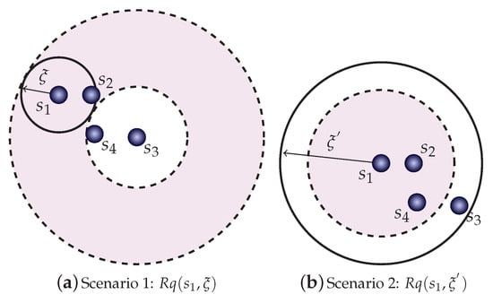
Figure 1.
Example of queries where the lower bound and the upper bound properties can be used to avoid unnecessary distance calculations.
Figure 1a shows a range query centered at element with radius . Notice that using element as a pivot, the calculation of the distance can be discarded by using the lower bound property. Although multiple pivots can be used to increase the “prunability”, as well as the positioning of pivots at the corner of the space, we keep this example with one pivot to indicate how to use the properties. In the example, every element outside the shaded area can be pruned, while those inside are considered false positives and must be investigated by calculating the real distance from the query center. Following our example dataset, the condition to avoid calculating distances from a given element to the query center using the lower bound property on pivot is then given by Equation (2):
The lower bound pruning is effective when dealing with small query radius , failing more often at higher values. This is because the proper formulation of the inequality uses to estimate the lower bound, once as higher the value of , higher the chance of the condition in Equation (2) fails. This situation leads to the scenario two, shown in Figure 1b, where a query with a larger radius is set. In this case, it is useful to use the upper bound property to detect coverage between the query ball and elements to search for. Now, it can detect if the query ball covers element , without the need to perform distance calculations to the query center . Following our example data set, the condition to avoid calculating distances from a given element to the query center using the upper bound property on pivot is given by the following. Elements detected inside the query ball can be directly added in the answer set without the verification of its distance from the query center. An element is covered by the query ball if
but, by the upper bound property on pivot , we derive
so it is safe to include if the following inequation holds:
Summarizing, we have now two support properties to aid similarity queries, one dedicated to prune elements from the query region (lower bound condition) and another dedicated to detect coverage of the query region (upper bound condition). Considering a query ball and a pivot , we can avoid calculation of , for all in the data set by using the following:
- Prune element
- Include element
However, we must consider that we can choose multiple pivots, and also the efficiency of each condition can be optimized by the position of each pivot in the data set. A pivot selection technique for this purpose is presented in the next section.
3.2. Maximizing Efficiency by Pivots Selection
The previously discussed properties can be optimized by a proper choice of the pivots. In this section, we propose one solution to choose pivots in order to maximize the prunability of the double pruning properties. Although the double pruning can be applied for any pivot, we intended to show that it is desirable to select them accordingly to obtain a higher chance of pruning success of each property. Therefore, we propose to select two types of pivots, the inner and outer pivots, each type associated with a pruning condition. The outer pivots are chosen for the usage of the lower bound property, and the inner pivots for the upper bound property.
For choosing the outer pivots, there are already studies that lead to the choice of elements at the corner (border) of the dataset, i.e., elements farthest from most of elements in the dataset [10]. This choice increases the efficiency of punning using the Equation (6). However, for inner pivots chosen for the upper bound property usage, we have to choose pivots in a different manner.
In order to increase the chance of satisfying the Equation (7), the left term can be minimized and the right term can be maximized, as an optimization problem. A directly but query dependent solution is by maximizing the right term, which is the radius value. Increasing radius on range joins will increase the chance of pruning using the upper bound property, which is a desirable effect on scalable joins. Another optimization possibility is to choose pivots nearest to the elements of the data set, minimizing in average the values of and , also minimizing the left term of Equation (7).
We propose one solution on how pivots can be selected attending the characteristics detailed above. Here, we choose pivots from a metric index created from both relations to be joined.
A Slim-tree is created from the relations to be joined, and this task can be performed offline before selecting pivots, once the Slim-tree is a disk-based metric tree. Since the elements stored on relations to be joined by similarity belong to the same metric space, the Slim-tree can index all elements of relations for the similarity join. The Slim-tree nodes group similar elements. Then, we take advantage of it to select proper pivots for each type of property.
Figure 2 shows an example of a tree-based index structure indexing features of elements from two relations to be joined, Relations and . The features must be from the same domain to be indexed in the same index. The index nodes of the structure will hold all node representatives hierarchically. They are good candidates to be elected as inner pivots because the representative elements have the smaller distance to their near elements, in average. On the other hand, the leaf nodes hold outer pivots candidates, excluding the elements from the first position of each leaf node (which are representatives on local node in Slim-tree).
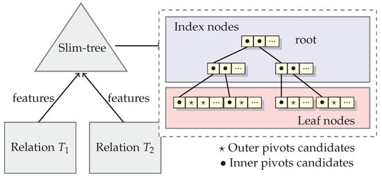
Figure 2.
Finding pivots candidates.
For the number of pivots, we follow the same idea of OMNI concept findings [10]. For the selection of outer pivots, we will follow the “Hull of Foci” (HF) algorithm on the OMNI concept. the HF algorithm randomly chooses an object , find the farthest object from , and set it as the first pivot. Then, it finds the farthest object from , setting it as the second pivot. The HF algorithm selects other pivots using a minimal error measure. Considering elements as the first chosen pivots, it searches for elements in order to minimize an error measure given by the following:
As the outer pivots candidates are stored in leaf nodes of the structure, excluding the first position of each leaf node, the list of outer pivots candidates is smaller and the algorithm will perform faster than the original OMNI strategy.
The task of selecting inner pivots is performed over the candidates list formed by index elements in the Slim-tree. In order to avoid selecting near pivots, the search must be performed in one tree level. For example, if the nodes in a same index level do not store the necessary number of candidates pivots, then the search will be performed entirely in the next level of the tree, until finding a suitable level.
The proposed technique can be applied to speed up any existing similarity search method. In this paper, we will illustrate an example of how our technique can be applied to resolve range joins, by applying it to the classical nested loop. Therefore, the next section shows the LUBJOIN algorithm, a simple nested loop join algorithm that uses our pruning technique. We will use it in experiments in order to analyze how the properties can be avoiding distance calculations.
4. Performing Similarity Joins
In the modern relational database management systems (RDBMSs), the information retrieval is performed by query operators, such as project, union, selection and join [28]. In Database theory, the join binary operator can be defined as a combination of other operators [17], as follows.
Definition 1 (Join operator).
The join of two relations and is a binary relational operator algebraically defined as a composition of two fundamental operators: a Cartesian product followed by the selection that perform the join predicate c:
When we bring this concept for a similarity scenario, the selection operator of a range join will refer to a similarity range selection, as:
Definition 2 (Similarity range selection).
The similarity range selection restricts the tuples of to those where the complex attribute is similar to considering a similarity threshold of ξ. It retrieves a subset such that .
Therefore, a range join will be defined according to the similarity range selection and the traditional join operator.
Definition 3 (Similarity range join).
The similarity range join combines the tuples of and whose distance between the pair of complex attributes is less than or equal to the given threshold ξ. It retrieves a set of pairs such that .
According to the definition, at high values of join radius , the answer set will also converge to the Cartesian product itself, which needs no distance calculations at this point.
As detailed in the previous section, we use the upper bound property from the metric to detect covering at high values of and the lower bound property to prune elements at low values of . In addition, in order to maximize the efficiency of the bounding properties, the inner and outer pivots must be properly defined following the process discussed in Section 3.2. Then, the pivots will be used for pruning and predicting.
The construction of the data structure for the new similarity join operator is performed in the following steps. Considering two relations and to be joined under a complex attribute, first the features are extracted into sets R and S within the same domain, respectively. The inner and outer pivots will be selected from an index composed of elements from both R and S. Then, the distances from pivots to elements of R and S are evaluated.
The algorithm of the proposed similarity join method is called LUBJOIN and it is described in Algorithm 1. The execution of the similarity join is performed in the following steps. For each element , a range query with radius will be executed over elements . The evaluation of each distance will be conditioned to the bounding conditions defined in Equations (6) and (7).
| Algorithm 1: LUBJOIN Algorithm |
| INPUT: Sets R and S, inner pivots , outer pivots , radius . OUTPUT: Result pairs () at .
|
5. Experiments
This section presents the results from experiments to evaluate our technique by using the proposed LUBJOIN algorithm. We performed range joins with different values of radius of the selection operator. The experiments were divided in two parts. In the first one, it was measured the efficiency of the proposed bounding properties. In the second, the performance of the LUBJOIN was evaluated in terms of number of distances calculated and time spent.
The performed range joins used a full range of values for the radius (updated to each data set) of the selection operator, in order to analyze the stability of our proposed technique to every possible radius value. The values for the radius were set up based on the evaluation of the diameter of the data set.
The LUBJOIN was compared with the traditional nested loop as the baseline, and also with one indexed table, in this case the Slim-tree as the index. It was not considered to filter the join result by eliminating repeated pairs of elements. The tests were performed on a computer with Pentium Intel Core i7 2.67GHz processor with 8 GB of RAM memory.
We used five data sets for the experiments. The description of each data set is shown in Table 2. The selected data sets allow exploring different types of data sets, varying the data set dimension, size, and type (geographic and images). The Corel data set consists of color histograms in a 32-dimensional space extracted from an image set. Using the distance, the maximum distance was rounded up to 3.28. The ImgTexture data set consists of Haralick textures in a 140-dimensional space extracted from an image set from the web. Using the Euclidean distance, the maximum distance was rounded up to 3670. The Points data set consists of a million random points in a six-dimensional space. Using the distance, the maximum distance was rounded up to 5.51. The USCities data set consists of Geographical coordinates (latitude and longitude) of USCities, villages, boroughs and towns. Using the spherical cosine distance, we considered to run at the maximum distance of 100 kilometers. the ImgMedical data set consists of color histograms formed by 256 grey levels from medical images. Using the distance, the maximum distance was estimated at 8740 and using the Mahalanobis distance estimated at 5245.
Table 2.
Data sets description used in experiments.
There are two initial approaches when selecting pivots. The first is to process a training set, for which it is usually a consistent subset of the entire data set. This setup speeds up the pivot selecting process once the training set is smaller than the entire dataset. However, the second approach is to dynamically update the current pivots set as new data is added to the dataset. Thus, if the new data is posed outside of the convex hull formed by the current pivots, they are updated using the linear time complexity algorithm [10,11]. In this paper, we assume the dynamical approach.
The construction process consists on selecting the pivots according to the approach detailed in Section 3.2. We used seven outer pivots and seven inner pivots selection in all experiments, which resulted in the best results compared to other tested quantities because the time spent increases if too many pivots are chosen. Although a high number of inner pivots may benefit the distance avoidance chance, the internal cost for this filtering stage can be higher than actually evaluating the distance. The cost of the construction relies on building the Slim-tree from the elements of both relations to be joined for pivots selection. We selected pivots from the candidates list produced by the index randomly. For simplicity, we considered the join relations as the same data set.
The first experiment evaluates the bounding properties filtering power. Similarity joins were performed varying the join radius from lower to higher values, but much smaller than the maximum distance in each data set. For the experiment, it was counted how many times each filter (lower or upper bound) successfully avoided the distance calculation. The results show which bounding property filters more elements according to the considered join radius, and bar plots show the proportion of each bounding property considering all successful prune operations.
Figure 3 shows a bars plot indicating the percentage of filtering that each condition holds for the Corel data set, for a range of values of the join radius. The full bar indicates 100% of the number of times that a distance evaluation could be avoided. From the plot, we can note that the lower bound condition filters most of the time at low values, while the upper bound condition filters at high values of the radius. Considering that the maximum distance in this data set is 3.28, we can see that the upper bound condition started to filter massively from radius 1.1 and on, compared to the lower bound condition. This indicates that the upper bound condition filtering power remains at high values of the join radius, avoiding unnecessary distance calculations.
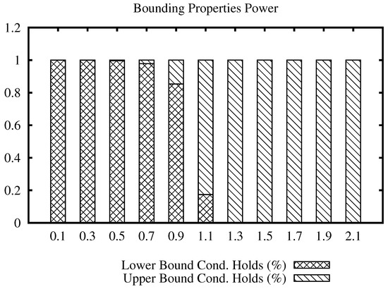
Figure 3.
Percentage of filtering that each bounding property can achieve within the range of radius of the join algorithm using the Corel data set.
Figure 4 shows the bars plot for the Images data set, for a range of values of the join radius. In this data set, we can note that the upper bound condition achieves more efficiency sooner at radius 1300, becoming the only property to filter after radius 2100, while the maximum distance in the data set is 3670.
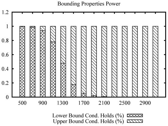
Figure 4.
Percentage of filtering that each bounding property can achieve within the range of radius of the join algorithm using the ImgTexture data set.
The bars plot for the Points data set is shown in Figure 5. While the maximum distance is 5.51, we can note that the transition of filtering power from the lower to upper bound condition occurs at radius 3. Beyond that, the upper bound condition maintains filtering elements at higher values of the join radius.
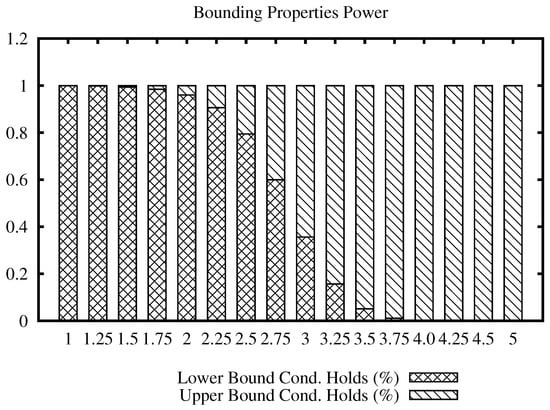
Figure 5.
Percentage of filtering that each bounding property can achieve upon the range of radius of the join algorithm using the Points data set.
The bars plot for the USCities data set is shown in Figure 6. From the plot, we can note that the upper bound property is the main active filter from radius value 80 and on.
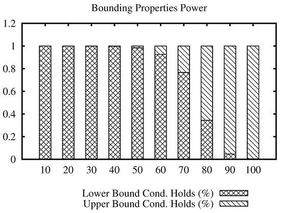
Figure 6.
Percentage of filtering that each bounding property can achieve upon the range of radius of the join algorithm using the USCities data set.
The bars plots for the ImgMedical data set are shown in Figure 7 and Figure 8. From the plot, we can see that the lower bound property filters mostly until radius 700 for the first and 400 for the second, and, from that value, the upper bound property filtering power increases.
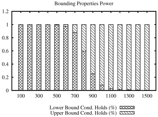
Figure 7.
Percentage of filtering that each bounding property can achieve within the range of radius of the join algorithm using the ImgMedical data set with the distance function.
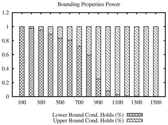
Figure 8.
Percentage of filtering that each bounding property can achieve within the range of radius of the join algorithm using the ImgMedical data set with the Mahalanobis distance function.
The previous results measured the efficiency of both properties to filter pairs of elements during a similarity join. The next experiment analyzes how many pairs of elements each property actually filters (prune) and how the similarity join performance can be improved by using our technique.
The next experiment measures the number of distance calculations and the time spent to perform similarity joins using the same data sets and values of radius. We evaluated the performance of the LUBJOIN against approaches such as the OMNI-sequential, Slim-tree (seq-Slim) and, for the small databases, we also calculated the statistics for the sequential scan (Seq-Seq). For comparison between properties of LUBJOIN, we also compared with a version where only the upper bound pruning is enabled. The selected range of values for the radius is different for each data set, according with the maximum estimated distance.
The results for the performance experiments on the data sets are shown in Figure 9 and Figure 10. Figure 9a,c,e and Figure 10a,c,e show the number of distance calculations needed to perform the similarity join, while Figure 9b,d,f and Figure 10b,d,f show the time measures.
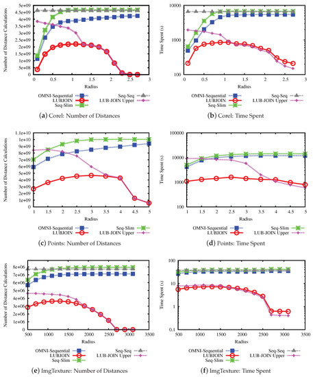
Figure 9.
Performance of similarity joins for LUBJOIN. (a,c,e) the average of the number of distances calculated in queries. (b,d,f) the time spent for performing the queries (milliseconds).
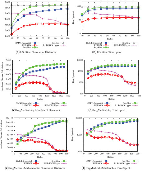
Figure 10.
Performance of similarity joins for LUBJOIN. (a,c,e) the average of the number of distances calculated in queries. (b,d,f) the time spent for performing the queries (milliseconds).
Considering the results, the first notable result is that the LUBJOIN reduced the number of distance calculations and time spent as radius value increases. This is because of the upper bound condition that filters more distances as the radius increases, as seen in the previous experiments. Another notable result is that using indexes like hierarchical balls of Slim-tree are ineffective when dealing with high radius values, due to the tree nodes overlap of the same level, and some cases causing it to perform more distance calculations than traditional sequential scan.
The results from experiments indicated that the LUBJOIN reduced the time spent when performing joins. However, in cases where the dataset dimension is low, as in the USCities dataset (Figure 10b), the computational cost of the distance is cheap and the quadratic traversing type of nested loops produced a major consumption of process time. Therefore, our technique can also benefit similarity operators that use non-cheap distance functions, which is the case of the Mahalanobis function on the ImgMedical dataset.
The last experiment measures the performance when varying the number of pivots in the LUBJOIN algorithm. A higher number of pivots may improve the performance when pruning with the upper bound property but not with the lower bound property, where the latter is related to the intrinsic dimension of the data set. The results are shown in Figure 11 and Figure 12. From the results, it can be seen that, in general, with a higher the number of pivots, the performance of pruning at high values of radius for the queries improve, but has little effect at lower values of radius.
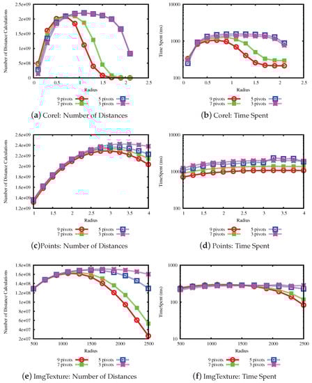
Figure 11.
Performance of similarity joins for LUBJOIN varying the number of pivots. (a,c,e) the average of the number of distances calculated in queries. (b,d,f) the time spent for performing the queries (milliseconds).
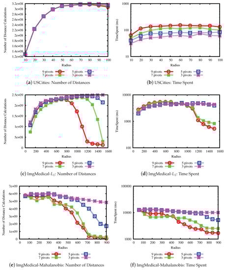
Figure 12.
Performance of similarity joins for LUBJOIN varying the number of pivots. (a,c,e) the average of the number of distances calculated in queries. (b,d,f) the time spent for performing the queries (milliseconds).
6. Conclusions
This paper proposed a double distance-calculation-pruning technique to improve similarity search. Metric bounding properties were applied on different scenarios optimizing the prunability of search algorithms. Different types of pivots were illustrated, the outer pivots and the inner pivots. Each pivot type enhances the chance to discard unnecessary distance calculations based on the lower or upper bound metric properties. An application example was proposed focusing on similarity joins, by the LUBJOIN algorithm.
Experiments on the filtering power of each property was performed in order to analyze how much they can avoid distances’ calculations. In addition, performance results showed that the LUBJOIN reduced the number of distance calculations and time spent to perform similarity joins, increasing its performance as the radius value increases.
The filtering conditions presented in this paper can be applied in any existing method to achieve scalable results. Thus, future works include applying those filtering conditions to well established methods in literature, or by proposing new strategies on choosing pivots.
Author Contributions
I.R.V.P. developed, implemented the proposed method and wrote the paper. D.M.E. provided datasets and structured the experiments. F.P.B.P. performed the experiments and discussed the results.
Acknowledgments
The authors would like to thank FAPESP (Fundação de Amparo à Pesquisa do Estado de São Paulo) for the financial support.
Conflicts of Interest
The authors declare no conflict of interest.
References
- Pola, I.R.V.; Cordeiro, R.L.F.; Traina, C.; Traina, A.J.M. Similarity sets: A new concept of sets to seamlessly handle similarity in database management systems. Inf. Syst. 2015, 52, 130–148. [Google Scholar] [CrossRef]
- Jacox, E.H.; Samet, H. Metric space similarity joins. ACM Trans. Database Syst. 2008, 33, 7:1–7:38. [Google Scholar] [CrossRef]
- Jousselme, A.L.; Maupin, P. Distances in evidence theory: Comprehensive survey and generalizations. Int. J. Approx. Reason. 2012, 53, 118–145. [Google Scholar] [CrossRef]
- Santini, S.; Jain, R. Similarity Measures. IEEE Trans. Patten Anal. Mach. Intell. 1999, 21, 871–883. [Google Scholar] [CrossRef]
- Bustos, B.; Navarro, G.; Chavez, E. Pivot selection techniques for proximity searching in metric spaces. Patten Recogn. Lett. 2003, 24, 2357–2366. [Google Scholar] [CrossRef]
- Ruiz, G.; Santoyo, F.; Chavez, E.; Figueroa, K.; Tellez, E. Extreme Pivots for Faster Metric Indexes. In Lecture Notes in Computer Science; SISAP ’13; Springer: Heidelberg/Berlin, Germany, 2013; pp. 115–126. [Google Scholar]
- Hetland, M. The Basic Principles of Metric Indexing. In Swarm Intelligence for Multi-Objective Problems in Data Mining; Studies in Computational Intelligence; Springer: Heidelberg/Berlin, Germany, 2009; pp. 199–232. [Google Scholar]
- Hetland, M.L.; Skopal, T.; Lokoc, J.; Beecks, C. Ptolemaic access methods: Challenging the reign of the metric space model. Inf. Syst. 2013, 38, 989–1006. [Google Scholar] [CrossRef]
- Brin, S. Near neighbor search in large metric spaces. In Proceedings of the 21th International Conference on Very Large Data Bases, San Francisco, CA, USA, 11–15 September 1995; Dayal, U., Gray, P.M.D., Nishio, S., Eds.; Morgan Kaufmann: Zurich, Switzerland, 1995; pp. 574–584. [Google Scholar]
- Traina, C., Jr.; Filho, R.F.S.; Traina, A.J.M.; Vieira, M.R.; Faloutsos, C. The Omni-family of all-purpose access methods: A simple and effective way to make similarity search more efficient. VLDB J. 2007, 16, 483–505. [Google Scholar] [CrossRef]
- Santos Filho, R.F.; Traina, A.J.M.; Traina, C., Jr.; Faloutsos, C. Similarity Search without Tears: The OMNI Family of All-purpose Access Methods. In Proceedings of the 17th International Conference on Data Engineering (2001), Heidelberg, Germany, 2–6 April 2001; IEEE Computer Society: Heidelberg, Germany, 2001; pp. 623–630. [Google Scholar]
- Dohnal, V.; Gennaro, C.; Savino, P.; Zezula, P. D-Index: Distance Searching Index for Metric Data Sets. Multimed. Tools Appl. J. 2003, 21, 9–33. [Google Scholar] [CrossRef]
- Gennaro, C.; Savino, P.; Zezula, P. Similarity Search in Metric Databases through Hashing. In Proceedings of the 3rd International Workshop on Multimedia Information Retrieval, Ottawa, ON, Canada, 5 October 2001; pp. 1–5. [Google Scholar]
- Indyk, P.; Motwani, R. Approximate Nearest Neighbors: Towards Removing the Curse of Dimensionality. In Proceedings of the Thirtieth Annual ACM Symposium on Theory of Computing, Dallas, TX, USA, 24–26 May 1998; ACM: New York, NY, USA, 1998; pp. 604–613. [Google Scholar]
- Chierichetti, F.; Kumar, R. LSH-Preserving Functions and Their Applications. J. ACM 2015, 62, 33:1–33:25. [Google Scholar] [CrossRef]
- Böhm, C.; Krebs, F. The k-Nearest Neighbor Join: Turbo Charging the KDD Process. Knowl. Inf. Syst. 2004, 6, 728–749. [Google Scholar] [CrossRef]
- Silva, Y.N.; Aref, W.G.; Larson, P.A.; Pearson, S.S.; Ali, M.H. Similarity Queries: Their Conceptual Evaluation, Transformations, and Processing. VLDB J. 2013, 22, 395–420. [Google Scholar] [CrossRef]
- Qin, J.; Zhou, X.; Wang, W.; Xiao, C. Trie-Based Similarity Search and Join. In Proceedings of the Joint Extending Database Technology and Database Theory International Conferences, Genoa, Italy, 18–22 March 2013; pp. 392–396. [Google Scholar]
- Wang, J.; Li, G.; Feng, J. Extending String Similarity Join to Tolerant Fuzzy Token Matching. Trans. Database Syst. 2014, 39, 7:1–7:45. [Google Scholar] [CrossRef]
- Xiao, C.; Wang, W.; Lin, X.; Yu, X.J. Efficient Similarity Joins for Near Duplicate Detection. Trans. Database Syst. 2011, 36, 15. [Google Scholar] [CrossRef]
- Chaudhuri, S.; Ganti, V.; Kaushik, R. A Primitive Operator for Similarity Joins in Data Cleaning. In Proceedings of the 22nd International Conference on Data Engineering (ICDE’06) (2006), Atlanta, Georgia, 3–7 April 2006; pp. 1–12. [Google Scholar]
- Zhang, C.; Li, F.; Jestes, J. Efficient Parallel kNN Joins for Large Data in MapReduce. In Proceedings of the International Conference on on Extending Database Technology, Berlin, Germany, 27– 30 March 2012; pp. 38–49. [Google Scholar]
- Silva, Y.N.; Reed, J.M. Exploiting MapReduce-based Similarity Joins. In Proceedings of the 2012 ACM SIGMOD International Conference on Management of Data, Scottsdale, AZ, USA, 20–24 May 2012; ACM: New York, NY, USA; pp. 693–696. [Google Scholar]
- Yu, C.; Cui, B.; Wang, S.; Su, J. Efficient Index-Based kNN Join Processing for High-Dimensional Data. Inf. Softw. Technol. 2007, 49, 332–344. [Google Scholar] [CrossRef]
- Liu, Y.; Hao, Z. A kNN Join Algorithm Based on Delta-Tree for High-dimensional Data. Comput. Res. Dev. 2007, 47, 1234–1243. [Google Scholar]
- Wang, Y.; Metwally, A.; Parthasarathy, S. Scalable All-pairs Similarity Search in Metric Spaces. In Proceedings of the 19th ACM SIGKDD International Conference on Knowledge Discovery and Data Mining, Chicago, IL, USA, 11–14 August 2013; ACM: New York, NY, USA, 2013; pp. 829–837. [Google Scholar]
- Faloutsos, C. Indexing of Multimedia Data. In Multimedia Databases in Perspective; Springer: Heidelberg/Berlin, Germany, 1997; pp. 219–245. [Google Scholar]
- Date, C.J. SQL and Relational Theory: How to Write Accurate SQL Code; O’Reilly Media, Inc.: Newton, MA, USA, 2011. [Google Scholar]
© 2018 by the authors. Licensee MDPI, Basel, Switzerland. This article is an open access article distributed under the terms and conditions of the Creative Commons Attribution (CC BY) license (http://creativecommons.org/licenses/by/4.0/).