AAC Double Compression Audio Detection Algorithm Based on the Difference of Scale Factor

Abstract

Audio dual compression detection is an important part of audio forensics. It is of great significance to judge whether the audio has been falsified and forged. This study found that the advanced audio coding (AAC) audio scale factor gradually decreases with the number of compressions increases. Based on this, we propose an AAC double compression audio detection algorithm based on the statistical characteristics of the scale factor difference before and after audio re-compression. The experimental results show that the algorithm can accurately classify dual compressed AAC audio. The average accuracy of AAC audio classification between low-bit-rate transcoding to high-bit-rate is 99.91%, and the accuracy rate between the same bit rate is 97.98%. In addition, experiments with different durations, different noises, and different encoders also proved the better performance of this algorithm.

1. Introduction

In the era of mobile Internet [1], the popularization of mobile smart terminals and the continuous advancement of multimedia technology have made great changes in people’s daily lives. People can use mobile phones more conveniently to collect photos, audio and share them on the Internet. This multimedia information constantly penetrates into people’s lives, making it difficult to distinguish between true and false. In order to detect the authenticity and integrity of multimedia information, multimedia forensics technology has become one of the hot research issues in the field of information security [2].

Digital audio forensics technology is an important part of digital multimedia forensics technology, and audio double compression detection is one of the hot issues in audio forensics technology [3]. Currently on the market for multimedia devices, the audio files are saved in a compressed format. The use of audio editing or processing software to tamper with compressed audio content is accompanied by the creation of double compression. Therefore, audio double compression detection as a previous step in the authenticity assessment of digital content is a necessary condition for judging whether the audio has been falsified or forged [4].

In the MP3 audio double compression detection, Yang et al. [5,6] found that the MP3 audio MDCT coefficients have a significant change in the number of coefficients before and after compression, so that the proportion of the 1 value coefficient in all frequency coefficients is used as a distinguishing feature to realize the effective detection of MP3 audio with low bit rate transcoding to high bit rate. In addition, they studied and analyzed the coefficients of double compressed audio Modified Discrete Cosine Transform (MDCT) coefficients and applied Benford’s theorem in image steganalysis to apply to double compressed audio detection. Liu et al. [7] proposed a threshold to achieve single-compressed audio and dual-compressed audio classification by further analyzing the distribution of MDCT coefficients. The differences in the distribution of zero-valued coefficients in MDCT coefficients and the difference between smoothness and consistency of non-zero-valued coefficients were analyzed [8,9], which greatly improved the detection accuracy of low bit rate transcoding to high bit rate audio. However, the same bit rate compressed audio detection accuracy still needs to be further improved. T. Bianchi et al. [10,11] introduced the recompression correction principle in the image into the audio. The audio to be measured is decoded, the quantization parameters are extracted, the obtained PCM sample values are clipped and recompressed and coded using the extracted quantization steps. With the use of primary and secondary compressed audio, after the recompression correction, the MDCT coefficient distribution and the pre-correction distribution show different rules, which can effectively detect double-compressed MP3 audio. Ren et al. [12] used the difference in the distribution of Quantized Modified Discrete Cosine Transform (QMDCT) coefficients between recompressed calibration audio and test audio. They performed MP3 recompression audio detection and estimated the compressed audio source rate. In the aspect of AMR recompression audio detection, D Luo et al. [13,14] used a deep learning algorithm and most voting strategies to design decisions to detect double-compressed AMR audio. In their further work, a dual-compression AMR audio detection framework based on the stacked automatic encoder (SAE) network, and the universal background model-Gaussian Mixture Model (UBM-GMM) is proposed.

In advanced audio coding (AAC) audio double compression detection, Jin et al. [15] combined the probability of occurrence of the Huffman code table index with its Markov one-step transition probability and used LIBSVM to classify single and double compressed AAC audio. Its detection rate of compressed audio at the same code rate is low. Li et al. [16] found that the AAC audio frequency components and energy values differ greatly during the compression process and use the Stacked Automatic Encoder (SAE) to detect double-compressed audio.

Through the research, it is found that in the AAC audio compression process, the audio scale factor decreases with the increase of the compression times. Based on the difference in the statistical characteristics of the scale factor before and after audio re-compression, we propose an AAC dual compression audio detection algorithm based on the difference of the scale factor. This algorithm combines the probability of difference of the scale factor and the mean value of the differences together as a detection feature. The LIBSVM is used to classify the recompressed AAC audio. Experiments were performed under different durations, different noises, and different encoders. The results show that the proposed algorithm has high detection accuracy and can effectively detect AAC dual-compressed audio.

2. AAC Audio Scale Factor Characteristics Change Analysis

2.1. Scale Factor in AAC

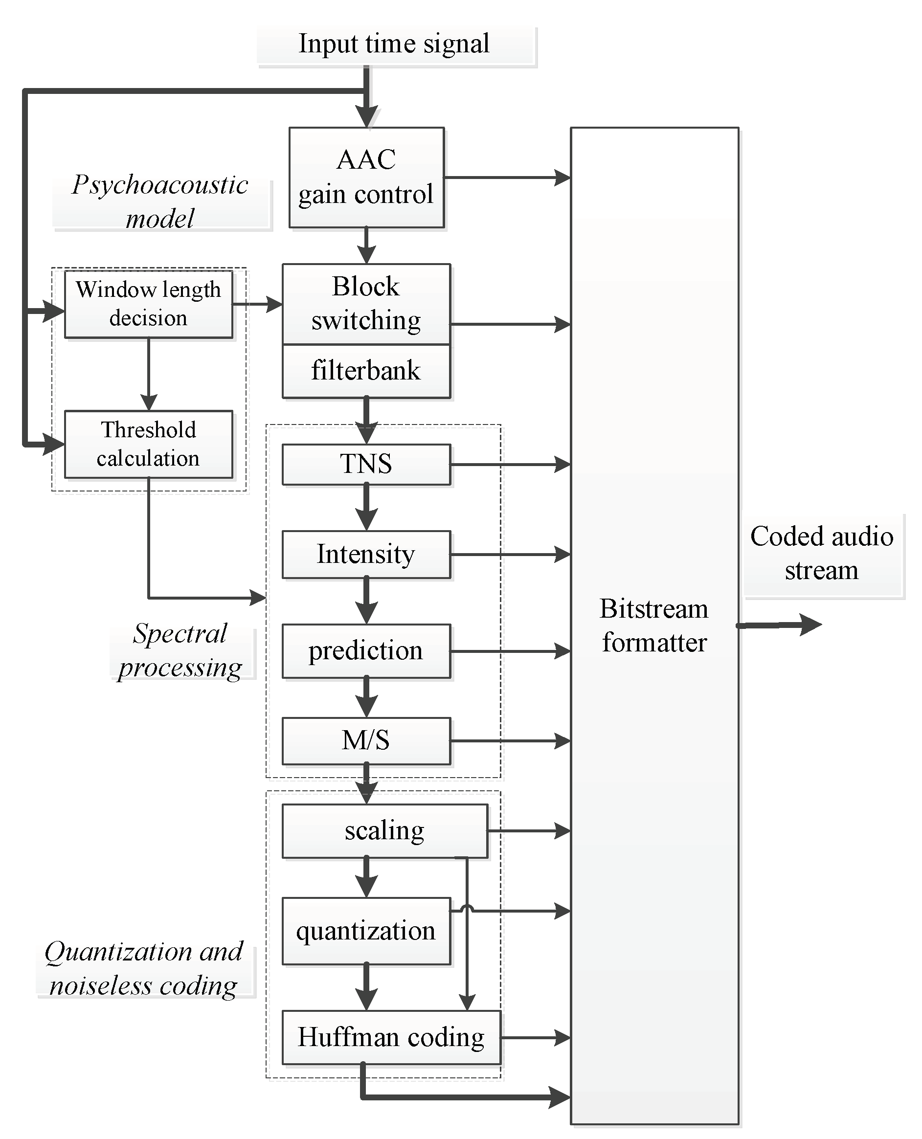
AAC is an abbreviation of Advanced Audio Coding [17] and is developed based on perceptual audio coding as a basic model. The coding block diagram is shown in Figure 1, and the coding process is as follows. The input PCM signal is time-frequency converted via a filter bank (filter lossless operation). Combined with the psychoacoustic model, the transformed frequency coefficients are quantized and encoded via MDCT processing. Finally, the encoded bit stream is encapsulated to form the final AAC compressed audio.

The AAC encoding is in frames, each frame contains two particles, for two channels each particle contains two channels, for a mono channel each particle contains one channel. Each channel produces 1024 coefficient values after the MDCT transform. AAC has 4 types of transform blocks in MDCT transform: long window block, short window block, start block and end block [18]. The long block is used for a relatively smooth data block in the time domain sample signal, the short block is used for a relatively severe block, and the start block and end block are used as transition block types. It should be noted that in our algorithm, we mainly focus on coding in the case of long window blocks.

After the MDCT transformation, the most important link is the iterative loop. In the iterative loop, some noise or high frequency information that people cannot hear will be filtered out. The purpose of the inner loop is to adjust the quantization step size, so that the number of bits of the quantized data after Huffman encoding can satisfy the number of bits required by the current encoding parameters. The quantization function in the inner loop of the AAC encoding is

$$x_{quant}=int\left({\left(\left|mdc{t}_{line}\right|\times 2^{\frac{1}{4}\left(s{f}_{decoder}-100\right)}\right)}^{\frac{3}{4}}+0.4054\right)$$

(1)

$int( )$ is a rounding down function, $s{f}_{decoder}$ represents a quantization step size, and $mdc{t}_{line}$, $x_{quant}$ are the spectral coefficients before and after quantization.

Adjusting the quantization step size in audio coding will adjust the scale factor representation range to control the quantization distortion of each scale factor band within the maximum allowable distortion range. The reduction in the scale factor is due in part to the increase in the quantization step size [19]. The high-frequency signal components in the audio have lower energy values. To preserve the accuracy of high-frequency signals, we use smaller quantization steps in the encoding process. After the audio undergoes the compression operation again, the high frequency information is relatively quantized to a value of 0 [20]. Compared with the first compressed audio, the quantization step length is increased, and the scale factor is reduced. By comparing the quantization steps and scale factors of the primary compression and the secondary compression, we believe that the quantization step can reflect the change of each frame of the audio to a certain extent. The scale factor can be used as the feature of AAC double compression audio detection.

2.2. Analysis of Changes in the Characteristics of the Scale Factor

In this algorithm, the default AAC compressed audio has the following two types: (1) low-bit-rate transcoding to high-bit-rate AAC audio, which is often referred to as false-quality audio, and the audio quality of poor audio quality (low-rate) is heavy to form false high-quality (high-rate) audio, and (2) same-bit-rate compressed AAC audio, which is usually an audio tamper recompressed to the original audio format with the same bit rate in order to prevent tampering and other operations from being discovered. For AAC audio with high bit rate transcoding to low bit rate, its meaning in the context of forensics has not been raised, this paper will not discuss. It is worth noting that the AAC compressed audio referred to herein refers only to compressed audio that has experienced two or less times.

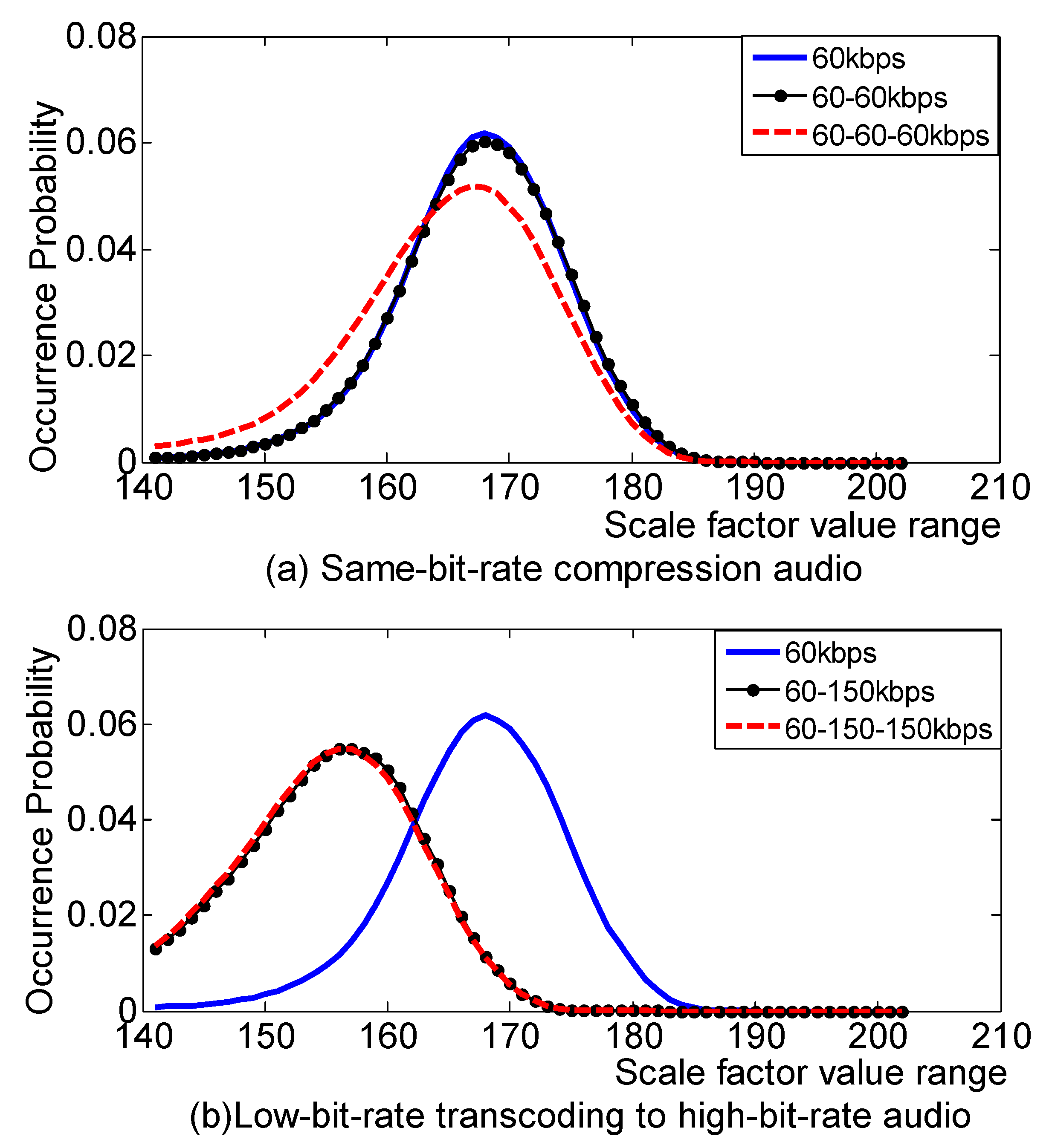
To analyze the changes in the AAC audio scale factor, we now randomly select 500 segments of 10 s of WAV audios including various styles such as classical, rock, folk, and pop. We compressed the 500 segments of WAV audios to get AAC first compression audio at 60 kbps and 150 kbps, and then processed the compressed AAC audio to obtain 60 → 60 kbps and 60 → 150 kbps secondary compressed audio. The decoding and encoding operation of the secondary compressed audio results in third compressed audio of 60 → 60 → 60 kbps and 60 → 150 → 150 kbps. Now we extract the scale factor of AAC audio for each compression case and count the information. The scale factor for AAC audio is in the range (0, 255). The value distribution is approximately Laplacian, and the result is shown in Figure 2. In this algorithm, in order to reduce the experimental dimension, we only take the distribution range of the main values of the scale factor in the statistical analysis (140, 200). From Figure 2, we can see that the probability of scale factor decreases with the increase of audio compression times. Through the comparison, it is considered that the AAC double compression audio can be detected by increasing the compression times of the audio to be measured and using the statistical characteristics of the change of the scale factor before and after the audio recompression.

3. Feature Construction and Extraction

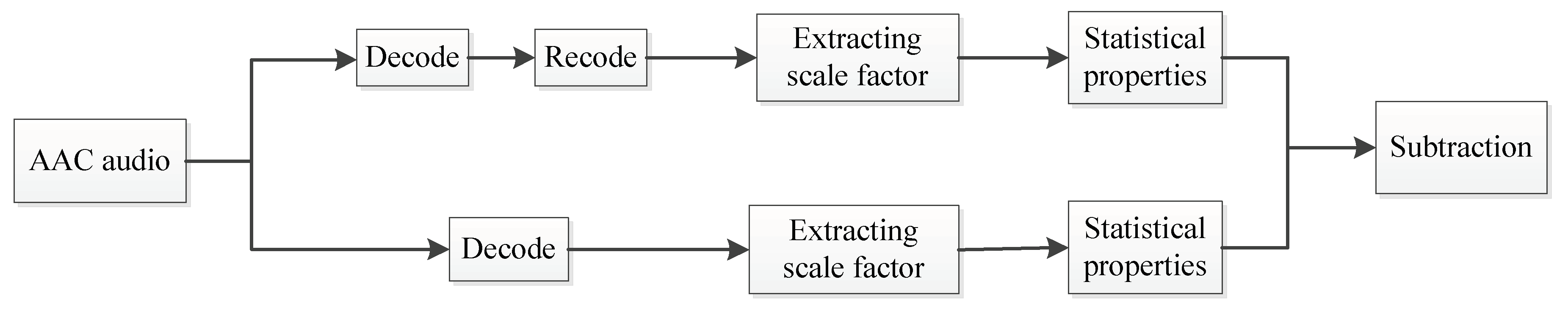
As can be seen from Figure 2, with the increase of compression times, the AAC audio scale factor will be relatively reduced. With this property, the difference between the audio recompressed audio and the original audio scale factor is used as a feature for detecting AAC audio double compression. Figure 3 is a feature extraction flow chart. For the AAC audio to be measured, two operations are performed on it. First, we directly extract the scale factor. Second, the AAC audio to be measured is decompressed, recompressed once with the same compression code rate to obtain the recompressed AAC audio, and the scale factor is re-extracted. The statistical information of the two scale factors is analyzed, and the difference characteristics are used as the final detection features. The AAC audio to be measured and recompressed is denoted as $M1,M2$, and the extracted scale factor matrix is denoted as $\mathrm{S}F1,\mathrm{S}F2$. The definition is as follows:

$$SF1=\left[\begin{array}{ccc}s{f}_{1,1}& \cdots & s{f}_{1,n}\\ ⋮& \ddots & ⋮\\ s{f}_{m,1}& \cdots & s{f}_{m,n}\end{array}\right]$$

(2)

$$SF2=\left[\begin{array}{ccc}s{f}_{1,1}{}^{\text{'}}& \cdots & s{f}_{1,n}{}^{\text{'}}\\ ⋮& \ddots & ⋮\\ s{f}_{m,1}{}^{\text{'}}& \cdots & s{f}_{m,n}{}^{\text{'}}\end{array}\right]$$

(3)

$n$ represents the number of scale factor bands. If it is a mono $m=2I$, if it is a dual-channel $m=4I$, $I$ represents the total number of audio long window frames to be measured.

3.1. Probability Difference Characteristics

The scale factor decreases as the number of audio compression increases, and its appearance probability will change accordingly as the number of compressions increases. Set the scale factor serial number to $k$. According to the above analysis, the value is mainly concentrated in (140, 200), and it is approximately a Laplacian distribution. Let us denote the probabilities of the scale factors of $M1$, $M2$ as $P_{SF1},P_{SF2}$

$$P_{SF1}=[P_{SF1}\left(k\right)|140\le k\le 200]$$

(4)

$$P_{SF2}=\left[P_{SF2}\left(k\right)|140\le k\le 200\right]$$

(5)

$P_{SF1}\left(k\right)$, $P_{SF2}\left(k\right)$, respectively, represent the ratio of the number of the scaling factor $k$ in $SF1$, $SF2$ to the total number of scale factors. Then, the probability difference between the scale factor of the test audio and the re-compressed audio is extracted, denoted as $\Delta p\left(k\right)$.

$$\Delta p\left(k\right)=P_{SF2}\left(k\right)-P_{SF1}\left(k\right)$$

(6)

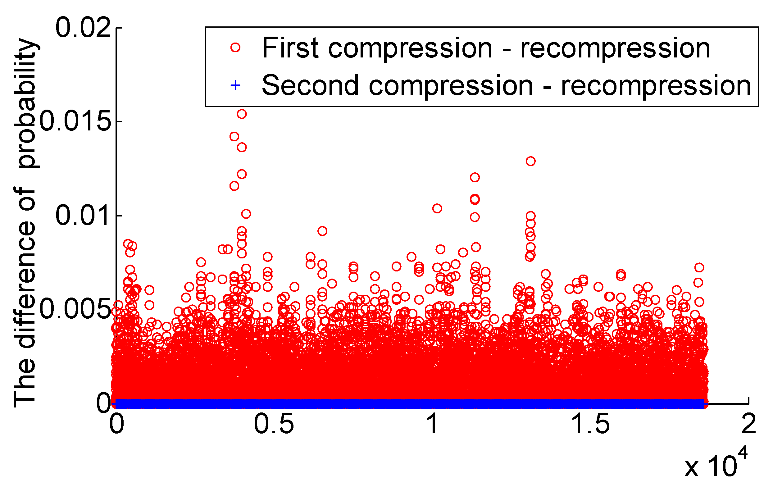
For convenience of description, the scale factor probability difference characteristic is denoted as $SFPD$. Randomly choose 300 segments of 10 s WAV audios, which include a variety of styles such as classical, rock, folk, popular, and so on. The first compressed AAC audio of 120 kbps is compressed for the 300 segments of audios, and the compressed audio is decompressed and recompressed to obtain 120 → 135 kbps secondary compressed audio. For the first and second compressed audio, we compress it again at the same code rate. Calculate the scale factor of AAC audio in each case and calculate the difference between the probability of occurrence of the scale factor of the first compressed audio and its recompressed audio $\Delta p_1\left(k\right)$ and the difference of the probability of occurrence of the scale factor of the second compressed audio and its recompressed audio $\Delta p_2\left(k\right)$. The Figure 4 is a scatter plot of the probability of occurrence of the scale factor difference $\Delta p_1\left(k\right),\Delta p_2\left(k\right)$. In the figure, “o” and “+” respectively represent $\Delta p_1\left(k\right),\Delta p_2\left(k\right)$. It can be seen that if the “o” distribution is more discrete, the value is larger, and if the “+” distribution is more concentrated, the value is smaller. The distribution distinction is more obvious, and we think it can be used for AAC double compression audio detection.

3.2. Characteristics of Average Difference

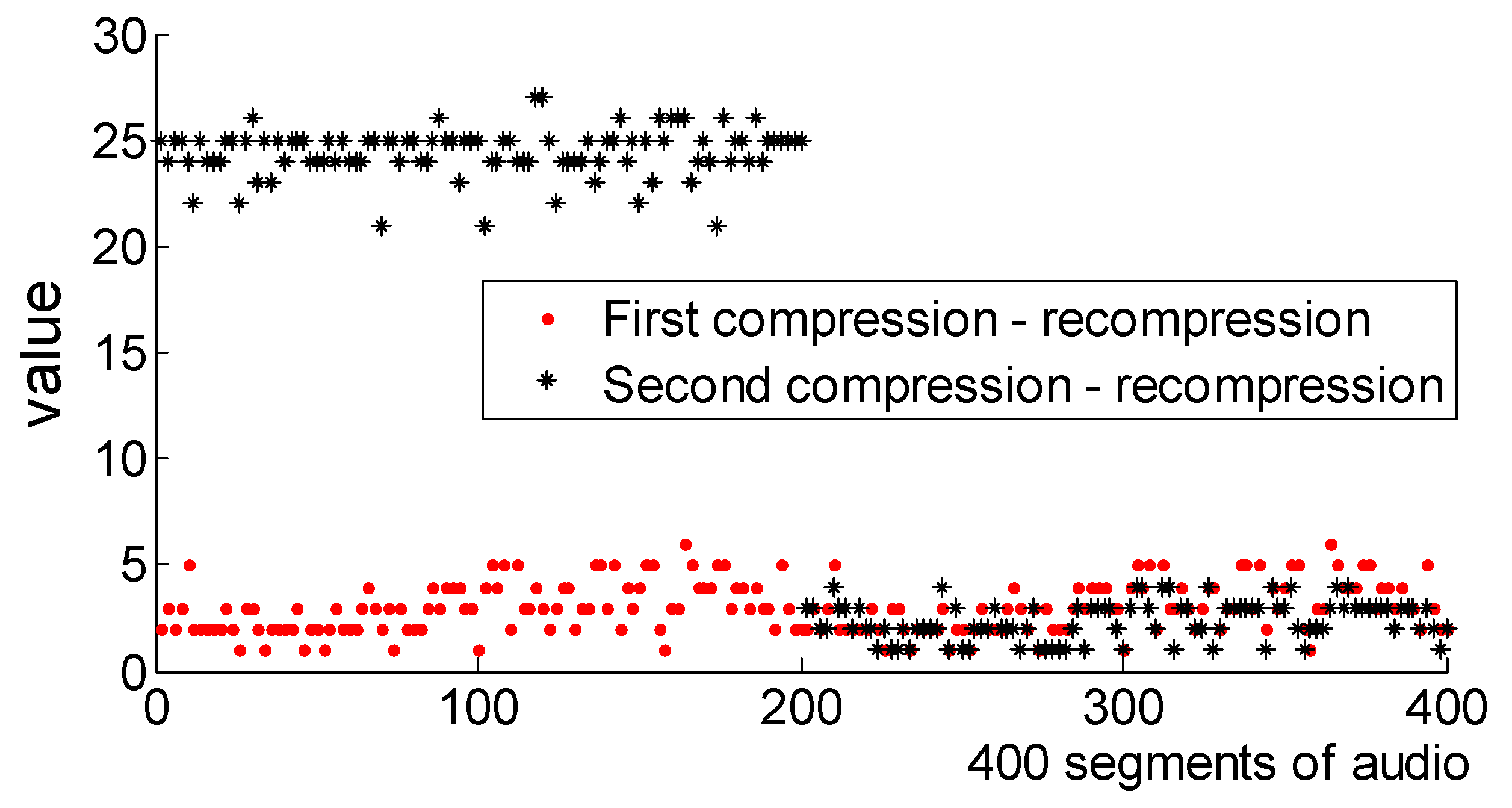
The variation law of the scale factor of the corresponding position after AAC audio first compression and second compression is not obvious. In order to highlight the differences, we extract the mean difference between the current AAC sample and the recompressed audio sample scale factor after decompression in the corresponding frame, which is denoted as $\Delta SF$.

$$\Delta SF=SF2-SF1=\left[\begin{array}{ccc}\Delta s{f}_{1,1}& \cdots & \Delta s{f}_{1,n}\\ ⋮& \ddots & ⋮\\ \Delta s{f}_{m,1}& \cdots & \Delta s{f}_{m,n}\end{array}\right]$$

(7)

For ease of description, the characteristic of the average value of the scale factor is denoted as $SFD$. Now we randomly choose 400 segments of audios, including 200 segments of once-compressed audios, re-compressed audio, and 200 segments of secondary-compressed audios, re-compressed audio. The secondary compressed audio includes 100 segments of same-bit-rate compressed audios and 100 segments of low-bit-rate transcoding to high-bit-rate audios. The mean value of the difference between the primary and secondary compressed and recompressed audio scale factors is denoted as $\Delta SF1$,$\Delta SF2$. The Figure 5 shows a scatter plot of 400 segments of audios averages. As can be seen, $\Delta SF1$,$\Delta SF2$ are more distinctive. In particular, the difference is very prominent. For the last 200 segments of AAC audios, the difference between encoding and decoding between the same-bit-rate audio compression is relatively small, the difference performance in Figure 5 is poor, but it can still be distinguished. Through analysis, it is considered that the average value of the scale factor difference can reflect the influence of the recompression scale factor globally, which can be used as an effective measure of AAC double compression audio.

4. Experimental Results and Analysis

4.1. Experiment Settings

We randomly selected 2000 segments of 10-s WAV audios as the original audio sample of this database. This 2000 segments of WAV audio contains various styles, such as blues, pop, classical, country, folk and so on. In this experiment, the AAC codec encodes and decodes audio using the most widely used open source software, FAAC-1.28 and FAAD2-2.7. The first compressed AAC audio is obtained by compressing 2000 segments of WAV audio of the above database using FAAC-1.28. A total of 2000 segments of (60, 75, 90, 120, 135, 150) kbps were obtained each. Secondary compressed audio is audio that is compressed once by FAAD2-2.7 and then encoded by FAAC-1.28. We have a total of 28 types of secondary compressed audios. For the above first and second compressed audio, the compression operation is performed again at the same-code-rate to obtain a re-compressed audio sample library.

This algorithm selects LIBSVM as a classifier and randomly selects 70% of the above samples for the training model and the remaining 30% as a test model. In order to make the test result more accurate, the detection accuracy in the paper is the average of the results after 10 repetitions of the experiment.

4.2. Feature Set $SFPD$ Feature Detection Results

Table 1. $SFPD$ detection accuracy—FAAC (%).

BR1	BR2
	60	75	90	105	120	135	150
60	94.33	97.67	98.67	99	97.17	99.5	97.17
75		93.96	98.33	99	97.67	99.33	98.67
90			94.67	97.33	98.5	99	97.83
105				90.33	99.5	98.67	98.76
120					92.83	100	98.33
135						90.5	97.58
150							92.13

shows the result of the detection of AAC audio by the $SFPD$. In the table, BR1 and BR2 indicate the audio compression code rate set in the first and second compression, and the values in the table represent the specific detection accuracy. Taking the 98.33% value of the seventh row and the eighth column of the table as an example, this value indicates that the method has achieved a combined detection rate of 98.33% for double-compressed AAC audio that uses 120 kbps and 150 kbps code rate compression (FAAC/FAAD2).

In Table 1, FAAC is an MPEG-4 and MPEG-2 AAC encoder. We can see that the average detection accuracy of low-bit-rate transcoding to high-bit -rate audio is 98.46%, and the same bit rate compressed audio detection is 92.67%. The $SFPD$ achieves better detection results at low-code-rate transcoding to high-code-rate. However, for the same bit rate of compressed audio, the detection rate is relatively low by about 5.79 percentage points, which is due to the relatively small change in the scale factor when the same-bit-rate audio is compressed. When the audio is compressed at the same code rate, the accuracy rate of (60, 75, 90) kbps is relatively higher than that when the code rate is (105, 120, 135, 150) kbps. The compressed code rate is high, the loss during compression will be relatively large. We use the difference in the probability of the scale factor after the audio recompression. It will reduce the difference between the primary and secondary compression characteristics.

4.3. Feature Set $SFD$ Feature Detection Results

Table 2. $SFD$ detection accuracy—FAAC (%).

BR1	BR2
	60	75	90	105	120	135	150
60	97.45	98.75	98.5	100	98.37	100	98.67
75		96.48	99.83	98.86	98	100	100
90			95.25	100	100	98.68	99.33
105				93.73	98.75	100	100
120					94.5	100	98.93
135						94.75	98.71
150							95.13

shows the detection result of the $SFD$ for AAC audio. The average detection accuracy of the low-bit-rate transcoding to high-bit-rate AAC audio is 99.3%, and the average accuracy rate between the same bit rate is 95.32%. From the table, we can see that $\mathrm{the}SFD$ achieves better detection results at low-bit-rates transcoding to high-bit-rates, and all exceed 98%. Similar to the $SFPD$, the detection rate is relatively low about 3.98 percentage points for compressed audio at the same code rate. From the comparison between Table 1 and Table 2, it can be seen that the $SFPD$ detection accuracy rate is lower than the $SFD$. It is considered that the AAC audio scale factor gradually decreases with the increase of the number of compressions, and its appearance probability also decreases relatively. It is more intuitive to use the difference of appearance probability of the scale factor to detect without directly using the scale factor difference.

4.4. Detection Results of Fusion Feature Sets

Insufficient detection of the same code rate double compression audio for feature set $SFD$ in the previous section. In combination with the construction method of feature set $SFPD$ in Section 4.2, this section improves the classification performance of the method at the same code rate by adding $SFPD$ statistical features to the $SFD$. Now we use the different weight ratios of $SFPD$ and $SFD$, update the fusion weights of different features iteratively, and finally use the fusion weights to classify the output of different feature sets. The iterative process is as follows.

(1) Different feature sets initialize the fusion weight coefficient $W_i$

$$W_i=\frac{1}{M},i=1,2,\dots M$$

(8)

$M$ is the number of different feature sets, here $M=2$, $W_i=0.5$ during initialization. That is, at the initial iteration, the $SFPD$ and $SFD$ are assigned a weight coefficient of 0.5.

(2) Iteratively updates $W_i$

Assume that the actual tag of AAC audio is $L\mathrm{able}\left(\mathrm{X}\right)$, $\mathrm{X}=0,1$. Where $\mathrm{X}=1$ means that the sample is a positive sample that is a single compressed AAC audio, and$\mathrm{X}=0$ represents that the sample is a negative sample that is double compressed AAC audio. And the classification tag of its feature fusion is $identity\left(X\right)$. If $Lable\left(X\right)=identity\left(X\right)$, the classification tag of feature fusion is compared with the classification tag of each feature. For sub-features that are judged to be incorrect (that is, the classification tag of feature fusion is inconsistent with the classification tag of sub-feature—$SFPD\mathrm{or}SFD$), the weight coefficient is subtracted from $\epsilon$, and the correct sub-feature is judged (that is, the classification tag of the feature fusion is consistent with the classification tag of the sub-feature—$SFPD\mathrm{or}SFD$), with the weight coefficient plus $\epsilon$. $\epsilon$ represents the error constant

$$\epsilon =\frac{ERR}{N}$$

(9)

$ERR$ indicates the integrated error rate of two sub-features when the classification is detected, and $N$ represents the total number of samples.

Get updated weight coefficient $W_i^{\ast }$

$$W_i^{\ast }=W_i\mp \epsilon$$

(10)

For the $SFPD$ and $SFD$ initial weight coefficients $W_1, W_2$ are 0.5, 0.5. For example, one AAC audio sample, the actual tag is $Lable\left(X\right)$, and the tagged note of its fusion feature set is$identity\left(X\right)$. If $Lable\left(X\right)=identity\left(X\right)$, we compare the fusion feature set classification results with the $SFPD$ and $SFD$ feature set classification results. Assume that for a certain AAC audio sample, the classification label of the fusion feature set is 1 and the classification label of the sub-feature set $SFPD$ is 0, and the weight coefficient $W_1$ is updated. $W_1=W_1-\epsilon$. In this case, in order to maintain the weight coefficient and always be 1, the weight coefficient $W_2$ of the $SFD$ is also updated accordingly, $W_2=W_2+\epsilon$.

If $L\mathrm{able}\left(\mathrm{X}\right)\ne \mathrm{identity}\left(\mathrm{X}\right)$, discard the sample, perform the above operation on the next sample, and repeat the above steps until all samples have been traversed. The resulting fusion feature set is recorded as $Featur{e}_{fusion}$

$$Featur{e}_{fusion}=W_1\ast SFPD+W_2\ast SFD$$

(11)

Table 3. $Featur{e}_{fusion}$ Detection Accuracy—FAAC (%).

BR1	BR2
	60	75	90	105	120	135	150
60	99.03	100	100	100	100	100	100
75		98.25	100	100	100	100	100
90			98.87	100	100	100	100
105				96.58	100	100	100
120					97.83	100	99.25
135						98.03	99
150							97.25

shows the detection accuracy of the fusion feature, $W_1$ = 0.463, $W_2$ = 0.537. The average detection accuracy of low-rate transcoding to high-rate AAC audio is 99.91%, and the average accuracy of same-rate compression detection is 97.98%. Table 3 compares Table 1 with Table 2 and finds that for the detection rate of AAC recompressed audio, the $Featur{e}_{fusion}$ further improves it. Compared with the $SFPD\mathrm{and}SFD$, the detection accuracy of AAC audio with low bit rate transcoding to high bit rate increased by 1.45 and 0.61 percentage points, respectively. Compared with the $SFPD\mathrm{and}SFD$, the detection accuracy of compression between the same-rate AAC audio increased by 5.31, 2.66 percentage points, respectively. The experimental results show that$Featur{e}_{fusion}$ integrates $SFPD\mathrm{and}SFD$ together well, which makes up for some deficiencies of the sub-feature set in AAC double compression audio detection.

In this paper, the first compressed AAC audio is a positive sample and the second compressed AAC audio is a negative sample. True Positives ($TP$) indicates that the positive class is positive, True Negatives ($TN$) indicates that the negative class is negative, False Positives ($FP$) indicates that the negative class is positive, and False negatives ($FN$) indicates that the positive class is negative class. The data in Table 3 is the accuracy of the test, that is, the ratio of the number of samples correctly classified by the classifier to the total number of samples for a given test data set.

$$ACC=\frac{TP+TN}{TP+FN+FP+TN}$$

(12)

The precision ($P$), which is for the prediction result, indicates that the prediction result is the number of positive samples that have positive samples. There are two possibilities for the prediction. One is to predict the positive class as a positive class ($TP$) and the other is to predict the negative class as a positive class ($FP$).

$$P=\frac{TP}{TP+FP}$$

(13)

The recall $\left(R\right)$ indicates the proportion of positive samples in the sample that are predicted correctly. There are two possibilities. One is to predict the positive class as a positive class ($TP$), and the other is to predict the original positive class as a negative class ($FN$).

$$R=\frac{TP}{TP+FN}$$

(14)

The $F\mathsf{\alpha }$ value is an evaluation index that combines the precision rate and the recall rate and is used to comprehensively reflect the overall indicators. When $\mathsf{\alpha }=1$, it is the most common $F1$ value.

$$F\mathsf{\alpha }=({\alpha }^2+1)\frac{P\ast R}{P+R}$$

(15)

Table 4. $Featur{e}_{fusion}$F1 value detection results—FAAC (%).

BR1	BR2
	60	75	90	105	120	135	150
60	94.63	96.58	97.63	96.87	98.57	97.25	98.54
75		93.32	98.06	95.42	96.93	98.67	95.86
90			94.59	97.38	98.43	96.33	97.89
105				93.87	97.93	98.43	98.67
120					94.02	95.67	97.33
135						95.63	96.5
150							92.15

shows the $F1$ values detected under the scale factor fusion feature set.

4.5. Comparison Test

In order to fully evaluate the performance of the algorithm proposed in this paper, this section reconstructs the features of Jin et al. [15] and conducts comparative experiments. The specific method of Jin feature construction is to use the Huffman code table to use the difference in single compression and double compression of AAC audio and take the probability of occurrence of the Huffman code table index as the first feature. The Markov one-step transition probability is taken as the second feature. The first feature is merged with the second feature and reduced in dimension to obtain the third feature. The LIBSVM is used to classify the single and double compressed AAC audio. Its low bit rate transcoding to high bit rate audio detection rate of 99.72%, the same bit rate audio compression detection rate of 77.38%.

Table 5. Comparison between [15] and the $Featur{e}_{fusion}$ of this algorithm—FAAC (%).

BR1	BR2 = BR3
	60	75	90	105	120	135	150
60	+21.37	0	0	0	0	0	0
75		+19.85	0	0	0	0	0
90			+23.62	+0.17	0	0	0
105				+25.36	+1.5	0	0
120					+20	+2.33	+0.1
135						+18.33	+0.57
150							+15.2

compares the result of the Jin method with the algorithm of this paper, where “+” indicates that the algorithm detection rate of the algorithm is higher than that of the Jin method detection rate, and “−” indicates that the detection rate of the algorithm is lower than the detection rate of the Jin method. It can be seen from Table 5 that the detection rate of the AAC audio Jin feature with low bit rate transcoding to high bit rate is high, which is not much different from that of the scale factor difference and occurrence probability difference in the algorithm of this paper. However, the detection effect between the same code rate in the literature [15] is poor. The algorithm in this paper solves similar problems and increases the detection rate of the same-rate compressed audio by nearly 20 percentage points. For a better comparison with this algorithm,

Table 6. Comparison between [15] and the $Featur{e}_{fusion} F1$ of this algorithm—FAAC (%).

BR1	BR2 = BR3
	60	75	90	105	120	135	150
60	+19.89	+0.13	−0.21	+0.05	−0.12	+0.34	+1.33
75		+20.35	+0.06	−0.1	+0.13	−0.16	−2.05
90			+20.16	+0.35	+1.21	+0.65	+0.56
105				+18.37	−1.2	0	−0.06
120					+20.03	+0.68	−0.37
135						+16.98	−0.31
150							+10.59

shows the comparison of $F1$ values between this algorithm and literature [15].

The AAC and MP3 codec are highly similar in principle. This section also reconstructs the features of the Yang et al. [6] method. It is worth noting that the Yang method is a typical method for detecting MP3 double compression. Its characteristic structure is as follows: the MDCT coefficients of 576 bands of MP3 audio are divided into 32 sub-bands on an average, and each sub-band contains 18 frequency line coefficients. The distribution of the first significant digits of each frequency band coefficient in the first 5, 10, 15 and 20 frequency bands is calculated (1~9). According to the Yang construction characteristics of the idea and the differences between MP3 and AAC, in this section, when reconstructing the Yang method, the first 10 frequency band coefficients are selected, and the first significant digits are counted. As a result, a 90-dimensional feature was constructed for each AAC sample.

Table 7. Comparison between [6] and the $Featur{e}_{fusion}$ of this algorithm—FAAC (%).

BR1	BR2
	60	75	90	105	120	135	150
60	+24.56	+30.03	+25	+5.03	0	0	+0.05
75		+11.48	+0.08	0	0	0	0
90			+20.05	−0.32	+0.05	0	+0.1
105				+20.97	+0.54	+0.22	+0.07
120					+22.21	+0.61	+0.22
135						+25.95	+1.43
150							+1.44

shows the accuracy of the modified Yang method for detecting AAC double-compressed audio.

The results in Table 7 show that the detection of AAC double compressed audio has a better detection result in the detection of low-bit-rate transcoding to high-bit-rate recompressed audio. The detection rate at the same-bit-rate compressed audio and 60 → 90 kbps, 60 → 75 kbps is lower. This algorithm solves the problem of poor detection rate, and the detection rate is significantly improved.

Table 8. Comparison between [6] and the $Featur{e}_{fusion} F1$ of this algorithm—FAAC (%).

BR1	BR2
	60	75	90	105	120	135	150
60	+21.35	+25.63	+15.68	+1.56	−0.32	+2.03	−0.11
75		+12.06	−0.26	+0.21	+0.09	+1.28	+0.35
90			+18.37	+0.51	+0.56	+0.35	0
105				+21.35	−0.05	−0.24	−0.21
120					+17.68	+1.65	−0.13
135						+26.35	+2.35
150							+5.68

shows the comparison of the $F1$ value of this algorithm compared with the literature [6].

4.6. Robust Experiment

4.6.1. Different Audio Duration Experiment Results

In the above experiments, the samples used were all 10 s AAC audio. To verify the performance of the algorithm in this paper, this section discusses the performance of the $Featur{e}_{fusion}$ at different times. AAC audio samples of different durations were obtained from 2000 segments of 10 s WAV audio in the above sample library. We cut out the WAV audio clips of 0.5 s, 1 s, 2 s, 3 s, 4 s, 5 s, 6 s, 7 s, 8 s, and 9 s and reproduced AAC audio sample libraries and re-compressed audio sample libraries of different durations. According to the above experimental process, the features of this paper were extracted, and the $Featur{e}_{fusion}$ was obtained.

Table 9. AAC dual compression detection accuracy at different durations—FAAC (%).

Duration (s)	Same-Rate Compression	Low-Bit -Rate Transcoding to High-Bit-Rate
0.5	78.56	91.56
1.0	82.35	93.33
2.0	87.63	95.12
3.0	91.33	95.89
4.0	94.87	97.85
5.0	96.05	97.63
6.0	97.14	98.58
8.0	97.02	99.03
9.0	97.89	99.87
10.0	97.98	99.91

shows the classification accuracy of the AAC audio double compression with the AAC audio at different durations. The same bit rate compression refers to the recognition rate when the bit rates of single and double compression are the same, and the low bit rate transcoding to high bit rate refers to the recognition rate when the second compression rate is higher than the first compression rate. As the audio duration increases, the detection accuracy of this algorithm also increases, indicating that the algorithm is still valid for AAC audio detection of different durations.

4.6.2. Experimental Results under Noise

In the 4.1 sample setup above, we randomly selected 2000 segments of WAV audio for 10 s. The WAV audio was clean audio. To further verify the robustness of this algorithm, this section discusses the performance of this algorithm in the case of noise addition. We added Gaussian white noise with different signal-to-noise ratios to 2000 original clean audio. We added noise with SNR of 0 dB, 10 dB, 15 dB, 20 dB, and 25 dB to recreate the sample library and re-compressed audio sample library. According to the above experimental process, the features of this paper were extracted, and the $Featur{e}_{fusion}$ was obtained.

Table 10. AAC double compression detection accuracy under noise—FAAC (%).

SNR	Same-Rate Compression	Low-Bit-Rate Transcoding to High-Bit-Rate
0 dB	92.35	98.33
10 dB	91.37	98.67
15 dB	90.05	97.45
20 dB	90.33	96.83
25 dB	87.67	95.31

shows the classification accuracy of AAC audio double compression with the fusion feature of AAC audio at different SNRs. At different signal to noise ratios, the detection accuracy of AAC audio double compression is still high, and when the signal to noise ratio is low, the accuracy rate is higher, indicating that the noise has little impact on the performance of the algorithm to a certain extent. This algorithm has better anti-noise performance.

4.6.3. Different Encoder Experimental Results

Although the same standard is followed for different encoders, there may be some differences in the specific implementation. To verify that the features selected in this paper are still valid for other encoders, this section selects another popular AAC codec, NeroAACCodec-1.5.1. According to Section 4.1 on the construction of the audio database, NeroAAC’s single-compressed audio is obtained by using neroAacEnc (encoder for NeroAACCodec-1.5.1) to compress 2000 segments of 10 s WAV audio, and then the compressed audio is decompressed by neroAacDec (decoder for NeroAACCodec-1.5.1) and then compressed by neroAacEnc into the corresponding dual-compressed audio. The recompressed audio of once and twice compressed audio is consistent with the above construction method. In the final training and testing, the used classifiers and classifier settings are the same as in Section 4.1.

Table 11. $Featur{e}_{fusion}$ detection accuracy—NeroAAC (%).

BR1	BR2
	60	75	90	105	120	135	150
60	90.13	96.3	89..12	90.45	94.65	99.3	98.27
75		80.35	85.33	89.56	96	98.98	98.32
90			87.47	93.56	97.9	97.03	97.66
105				83.22	98.67	97.35	99.27
120					80.45	96.79	97.77
135						80.65	93.56
150							84.33

shows the detection accuracy of NeroAAC double compressed audio using the $Featur{e}_{fusion}$. From the table, we can see that for the AAC audio of different encoders, the $Featur{e}_{fusion}$ still has a good detection accuracy. The double compressed audio performance of the feature set at low bit rate transcoding to high bit rate is still better than that at the same bit rate compressed audio. From the comparison of

Table 12. $Featur{e}_{fusion}$ detection accuracy—FAAC-NeroAAC (%).

BR1	BR2
	60	75	90	105	120	135	150
60	80.45	93.17	85.57	89.65	91.16	96	92
75		79.65	83.35	86.33	93.88	92.25	94.33
90			81.33	91.63	94.63	90.33	92.59
105				82.56	93.25	91.25	93.56
120					79.33	89.83	90.23
135						82.15	94.35
150							83

and Table 3, it is found that the $Featur{e}_{fusion}$ is more accurate in detection of FAAC double compressed audio than in NeroAAC. The analysis found that the change in the scale factor of the NeroAAC audio before and after the first and second compression is smaller than that of the FAAC audio Therefore, the detection rate of the NeroAAC audio is slightly lower when the scale factor feature is used for detection.

To further test the validity of the features presented in this algorithm, crossover experiments between different encoders were also performed in this section. That is, the following two cases are (1) compress the 2000 segments of 10 s WAV audios using FAAC-1.28 to obtain the once compressed audio, use FAAD2-2.7 to decompress it and then use neroAacEnc to compress the corresponding secondary compressed audios and (2) use neroAacEnc to compress 2000 segments of WAV audios to get compressed audios once. Use neroAacDec to decompress and then use FAAC-1.28 to compress the corresponding second compressed audio.

Table 12 and

Table 13. $Featur{e}_{fusion}$ Detection Accuracy—NeroAAC-FAAC (%).

BR1	BR2
	60	75	90	105	120	135	150
60	75.33	87.67	86	83.23	93.56	93.12	94.56
75		76.45	79.59	84.58	94	91.61	89.57
90			78.98	85.41	93.77	88.74	88.28
105				80	90.33	90.27	84.05
120					73.56	87.47	88.68
135						74.28	83.33
150							78.56

are the results of crossover experiments in the above two cases. Although the results of the crossover experiments between different encoders are significantly lower than the experimental results of a single encoder, it still has a certain detection effect. For FAAC-NeroAAC crossover experiments, the average recognition accuracy rate of low bit rate transcoding to high bit rate is 91.40%. The average recognition rate of the same-rate audio compression is 81.21%. For NeroAAC-FAAC crossover experiments, the average recognition accuracy of low bit rate transcoding to high bit rate is 88.94%. The average recognition rate of the same-rate audio compression is 76.74%. The $Featur{e}_{fusion}$ performs relatively well on low bit rate transcoding to high bit rate audio, but it has a large difference in the detection of some AAC double compressed audio. As shown in Table 12, the detection rate of double compressed audio for 60 → 135 kbps is 96%, while the detection rate for double compressed audio at 75 → 90 kbps is only 83.35%, which is nearly 12.65 percentage points lower. The same is true for Table 13, where the detection rate for double compressed audio at 60 → 150 kbps is 94.56%, while the detection rate for double compressed audio at 75 → 90 kbps is only 79.59%, which is nearly 14.97 percentage points lower.

From Table 3 and Table 11, Table 12 and Table 13, we find that there is a large difference in the detection rate of the $Featur{e}_{fusion}$ for the AAC double compressed audio of different codecs. Among them, the double-compression audio detection for the FAAC/FAAD2 processing by the codec has higher accuracy. Although the crossover results are lower than those of a single codec, the experimental results indicate that double compressed AAC audio can still be detected.

5. Conclusions

In this paper, an AAC double compression audio detection algorithm based on statistical characteristics of scale factor difference is proposed for recompressed AAC audio. By studying the change of the scale factor in the compression process, the double compression AAC audio is classified using the difference feature of the scale factor before and after the audio recompression. Experimental results show that the feature of this paper has better detection performance. The accuracy of AAC audio detection between low code rate transcoding to high code rate is 99.91%, and the detection accuracy rate between audio code compression rate of the same code rate is 97.98%. Experiments with different durations, different noises, and different encoders have proved that the proposed algorithm has strong robustness.

References

- Li, S.; Xu, L.D.; Zhao, S. 5G Internet of Things: A Survey. J. Ind. Inf. Integr. 2018, 10, 1–9. [Google Scholar] [CrossRef]
- Yang, R.; Luo, W.; Huang, J. Multimedia forensics. Sci. Sin. 2013, 43, 1654–1672. [Google Scholar]
- Yan, D.; Wang, R.; Zhou, J.; Jin, C.; Wang, Z. Compression history detection for MP3 audio. KSII Trans. Internet Inf. Syst. 2018, 12, 662–675. [Google Scholar] [CrossRef]
- Jin, C. Research on Key Technologies of Digital Audio Passive Forensics. Ph.D. Thesis, Ningbo University, Ningbo, China, 2016. [Google Scholar]
- Yang, R.; Shi, Y.Q.; Huang, J. Defeating fake-quality MP3. In Proceedings of the 11th ACM Multimedia Security Workshop, MMandSec’09, Princeton, NJ, USA, 7–8 September 2009; pp. 117–124. [Google Scholar] [CrossRef]
- Yang, R.; Huang, J. Detecting double compression of audio signal. In Media Forensics and Security II; SPIE: Bellingham, WA, USA, 2010; Volume 7541, p. 75410. [Google Scholar] [CrossRef]
- Liu, Q.Z.; Sung, A.H.; Qiao, M.Y. Detection of Double MP3 Compression. Cognit. Comput. 2010, 2, 291–296. [Google Scholar] [CrossRef]
- Qiao, M.Y.; Sung, A.H.; Liu, Q.Z. Improved Detection of MP3 Double Compression Using Content-Independent Features. In Proceedings of the IEEE International Conference on Signal Processing, Communication and Computing, Kunming, China, 5–8 August 2013. [Google Scholar]
- Qiao, M.; Sung, A.H.; Liu, Q. Revealing real quality of double compressed MP3 audio. In Proceedings of the ACM Multimedia 2010 International Conference, MM’10, Firenze, Italy, 25–29 October 2010; pp. 1011–1014. [Google Scholar] [CrossRef]
- Bianchi, T.; De Rosa, A.; Fontani, M.; Rocciolo, G.; Piva, A. Detection and localization of double compression in MP3 audio tracks. EURASIP J. Inf. Secur. 2014, 2014, 10. [Google Scholar] [CrossRef] [Green Version]
- Bianchi, T.; De Rosa, A.; Fontani, M.; Rocciolo, G.; Piva, A. Detection and classification of doublecompressed MP3 audio tracks. In Proceedings of the 2013 ACM Information Hidingand Multimedia Security Workshop, IH and MMSec 2013, Montpellier, France, 17–19 June 2013; pp. 159–164. [Google Scholar] [CrossRef]
- Ren, Y.; Fan, M.; Ye, D.; Yang, J.; Wang, L. Detection of double MP3 compression Based on Difference of Calibration Histogram. Multimedia Tools Appl. 2016, 75, 13855–13870. [Google Scholar] [CrossRef]
- Luo, D.; Yang, R.; Huang, J. Detecting double compressed AMR audio using deep learning. In Proceedings of the IEEE International Conference on Acoustics, Speech and Signal Processing, Florence, Italy, 4–9 May 2014; pp. 2669–2673. [Google Scholar] [CrossRef]
- Luo, D.; Yang, R.; Li, B.; Huang, J. Detection of Double Compressed AMR Audio Using Stacked Autoencoder. IEEE Trans. Inf. Forensics Secur. 2017, 12, 432–444. [Google Scholar] [CrossRef]
- Jin, C.; Wang, R.; Yan, D.; Ma, P.; Zhou, J. An efficient algorithm for double compressed AAC audio detection. Multimedia Tools Appl. 2016, 75, 4815–4832. [Google Scholar] [CrossRef]
- Li, X. Research on AMR and AAC Audio Dual Compression Detection. Ph.D. Thesis, South China University of Technology, Guangzhou, China, 2015. [Google Scholar]
- Institution, B.S. ISO/IEC 13838-7/FPDAM 1. Information Technology. Generic Coding of Moving Pictures and Associated Audio Information. Part 7: Advanced Audio Coding (AAC). Amendment 1: Signalling of Bandwidth Extension.
- Han, S.; Fingscheidt, T. Robust MPEG-4 high-efficiency AAC with fixed- and variable-length soft-decision decoding. In Proceedings of the 139th Audio Engineering Society International Convention, AES 2015, New York, NY, USA, 29 October–1 November 2015; p. 9399. [Google Scholar]
- Gao, Z.; Wei, G. The core technology of the broadband MP3 audio compression. Electroacoust. Technol. 2000, 9, 9–13. [Google Scholar]
- D’Alessandro, B.; Shi, Y.Q. MP3 bit rate quality detection through frequency spectrum analysis. In Proceedings of the 11th ACM Workshop on Multimedia and Security, Princeton, NJ, USA, 7–8 September 2009; pp. 57–61. [Google Scholar] [CrossRef]
Figure 1.
Advanced audio coding (AAC) framework.
Figure 2.
AAC audio scale factor occurrence probability.
Figure 3.
Feature extraction flow chart.
Figure 4.
Distribution of probability difference of audio and recompression audio scale factor.
Figure 5.
Randomly select the mean of the difference between 400 AAC audio.