An Improved Genetic Algorithm with a New Initialization Mechanism Based on Regression Techniques

Abstract

Genetic algorithm (GA) is one of the well-known techniques from the area of evolutionary computation that plays a significant role in obtaining meaningful solutions to complex problems with large search space. GAs involve three fundamental operations after creating an initial population, namely selection, crossover, and mutation. The first task in GAs is to create an appropriate initial population. Traditionally GAs with randomly selected population is widely used as it is simple and efficient; however, the generated population may contain poor fitness. Low quality or poor fitness of individuals may lead to take long time to converge to an optimal (or near-optimal) solution. Therefore, the fitness or quality of initial population of individuals plays a significant role in determining an optimal or near-optimal solution. In this work, we propose a new method for the initial population seeding based on linear regression analysis of the problem tackled by the GA; in this paper, the traveling salesman problem (TSP). The proposed Regression-based technique divides a given large scale TSP problem into smaller sub-problems. This is done using the regression line and its perpendicular line, which allow for clustering the cities into four sub-problems repeatedly, the location of each city determines which category/cluster the city belongs to, the algorithm works repeatedly until the size of the subproblem becomes very small, four cities or less for instance, these cities are more likely neighboring each other, so connecting them to each other creates a somehow good solution to start with, this solution is mutated several times to form the initial population. We analyze the performance of the GA when using traditional population seeding techniques, such as the random and nearest neighbors, along with the proposed regression-based technique. The experiments are carried out using some of the well-known TSP instances obtained from the TSPLIB, which is the standard library for TSP problems. Quantitative analysis is carried out using the statistical test tools: analysis of variance (ANOVA), Duncan multiple range test (DMRT), and least significant difference (LSD). The experimental results show that the performance of the GA that uses the proposed regression-based technique for population seeding outperforms other GAs that uses traditional population seeding techniques such as the random and the nearest neighbor based techniques in terms of error rate, and average convergence.

1. Introduction

Genetic algorithms (GAs) are stochastic optimization search techniques that depend on the natural evolution strategies. GAs strategies are based on the concept of ‘survival of the fittest’. The basic principles of GAs were first described at the University of Michigan in the 1970s by John Holland [1]. Holland aimed to simulate the natural evolution by studying the adoption in natural and artificial systems [2]. Holland introduced GAs from Darwinian theory ‘survival of the fittest’ [3,4], by generating new generation, chromosomes, through recombination (crossover) and mutation operations, then the fittest or feasible individuals are more likely to remain, mate and generate a new generation. The new individuals need to have more favorable fitness than the previous ones (i.e., the solution evolves from one generation to another). However, this is not the case all the time, as the new individuals may have worse fitness than the previous ones as well, but this can be solved using a good selection strategy.

GAs are often suitable to achieve the optimal or near-optimal solution for big or huge search space problems [5,6]. They are not a mathematically guided algorithm; however, they are a stochastic algorithm where generation and selection are implemented randomly [7]. Having two major operators, crossover and mutation allows GAs to deal with optimization problems efficiently, where the crossover operator attempts to create better solutions from in-hand solutions, and the mutation operators allows GAs to overcome strong local minima [8]. Therefore, GAs continue to attract the interest of many researchers as optimization tools for solving many problems to find the optimal or near-optimal solution quickly, reliably, accurately, and effectively [9,10,11]. Thus, they became popular techniques for solving wide variety of problems such as image processing [10], speech recognition [12,13], software engineering [14], clustering low-dimensional data [15], optimization of transport networks [16], vehicle detection [17], business process simulation [18], sensor network configuration [19], and robotics [20]. GAs has been developed to increase the population diversity and the efficiency to find the solution [21]. Therefore, new types of the standard GAs have emerged such as multi-population GAs and parallel GAs.

The initial population seeding phase is the first phase of any GA application. It generates a population of feasible solutions or individuals randomly or by heuristic initialization as input for the GA. Although the initial population seeding phase is executed only once, it has an important role to improve the GA performance [22,23]. While the others GA phases are repeated [24,25]. A various initialization techniques have been introduced since the emergence of GAs concepts. All of known techniques depend on the availability of information about the problem being studied [24,26]. The random initialization technique is considered as one of the most appropriate and commonly used technique to generate the initial population seeds. Random technique contains poor fitness solution that decreases the possibility of finding the optimal solution or near to optimal; also it requires long searching time in the case of deficient knowledge. However, the random population is preferred when applying GAs on various problems. On the other hand, in huge search space, if the preceding heuristic information about the optimal solution is available, then it can generate the initial population and recognize high quality solution areas easily. The process of generating initial population seeding using heuristic techniques implies high quality of population individuals that allows GAs to find the better solutions faster. However, it may end up with a small search space region and may never be able to obtain the universal optimal solutions [27].

Usually, the computation time of GAs to extract the initial population seeding is less than the computation time consumed for normal generation process. Further, the populations in each recursive generation process depend on their previous populations and at the end on the initial population seeding [25]. Therefore, specifying the initial population in GA is very important to decrease the computation time and then to find the optimal/near-optimal solution. The initial population seeding is as important as the other GA’s phases; it plays a manifest role in increasing the efficiency, also to obtain the optimal solution or the nearest to optimal. But, the random initialization technique generates a population of individuals that need additional computation time to obtain the optimal or near to optimal solution because of their infeasible and bad quality status. Researchers declared the need to improve the quality of population that is generated at the initial population stage of GA. Additionally, the improved convergence rate is very important requirement for solving particular problem. They pointed that the GAs may obtain the optimal solution for a given problem when generating the initial individuals with good quality and maximum diversity [28]. The individuals in each generation depend on the previous generation and finally on the initial population [29]. Researchers proved that the initial population seeding that depends on a prior knowledge about the problem can enhance GA’s capability to provide solutions near to an optimal solution [26].

The used method to generate the initial population has a critical impact on determining the convergence speed and the quality of provided solution [30]. The specific initial population seeding technique for a problem improves the efficiency of GAs to find the optimal solution, and the proposed techniques for the initial population seeding are limited [31]. Most of these techniques focus on the quality improvement of the initial population seeding such as: random, nearest neighbor, and K-means clustering, see Figure 1. The limited number of these techniques motivates this study, as there is still room for enhancing and finding better initial population to start with.

There are several various factors that could influence the performance of GAs: parameters, genetic operators and strategies [34]. One of the main factors that effect on GAs performance is the initial population. Random initial population is considered as a traditional method for obtaining the initial population, however it is inefficient to produce a favorable initial population usually. This work proposes a new initial population technique based on regression for GAs initial population. Our experiments showed promising results in improving the GAs performance to solve TSP. We analyze the performance of the GA using traditional population seeding techniques, such as the random and nearest neighbors, along with the proposed regression-based techniques. Our approach divides the problem into sub problems using the regression line analysis that displays the relationship between the points in $x-y$ coordinates. The partition occurs because of the intersection of regression line and the perpendicular line at the center point. This allows for clustering the cities into four sub-problems repeatedly, the coordinates of each city determines which category/cluster the city belongs to, the algorithm works repeatedly until the size of the subproblem becomes very small, four cities or less for instance, these cities are more likely to be adjacent to each other, so connecting them to each other creates (somehow) a good solution to start with, this solution is mutated several times to form the initial population.

Our experiments show promising results that highlight the efficiency of our new approach in terms of improvement in error rate, average convergence and convergence diversity. The contributions of this work include a new approach for producing initial population in the case of solving TSP problem compared to Random, NN techniques.

The rest of this paper is organized as follows. Section 2 reviews the basics of GA, solving TSP using GA along with highlighting important population seeding techniques. Section 3 introduces our regression-based technique with illustrative example. Section 4 provides detailed experimental results on TSP and compares with different techniques with different error metrics. Finally, Section 5 concludes the paper indicating possible future research directions.

2. Background

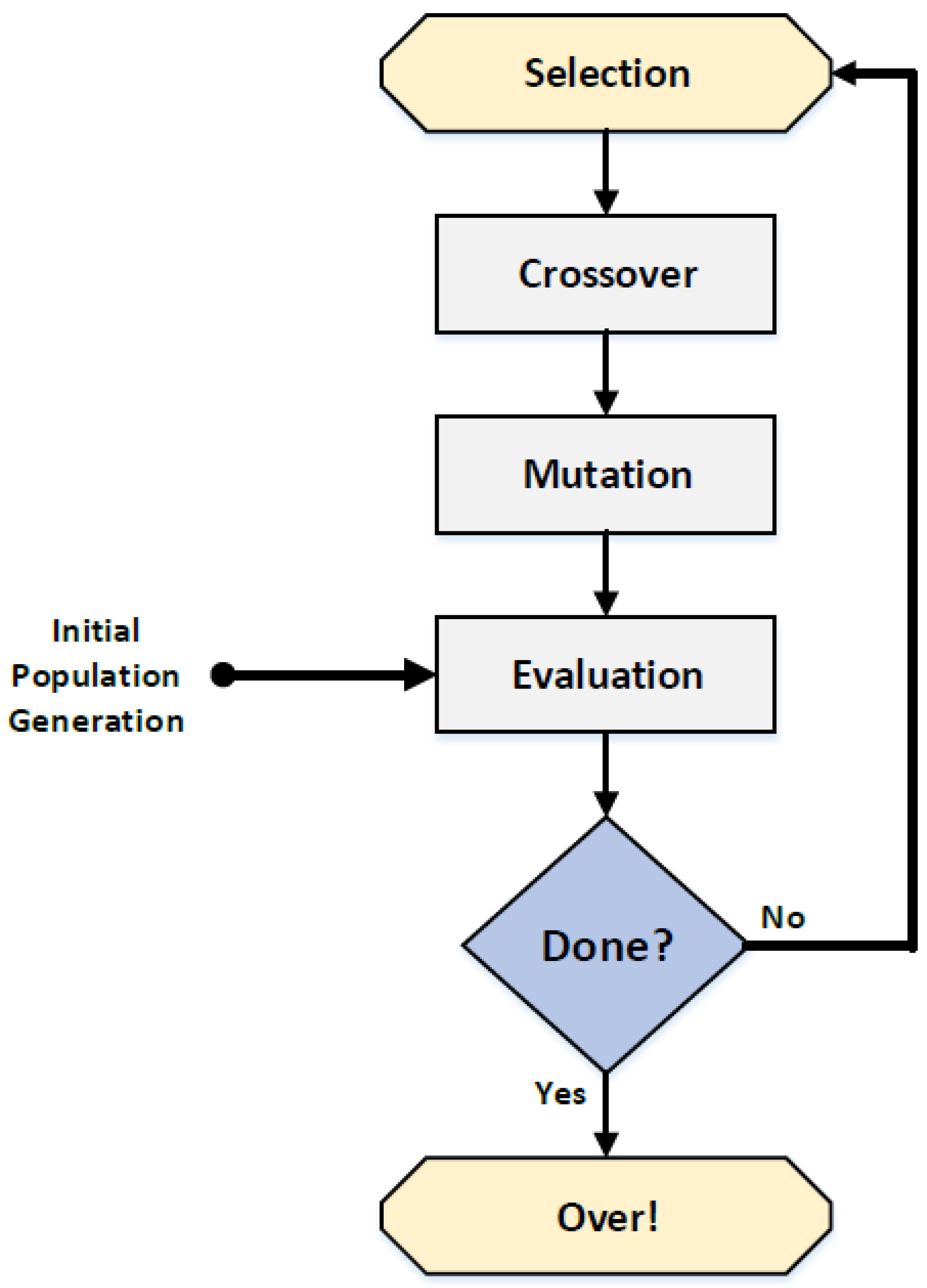
2.1. Basic Principles of Genetic Algorithms

GA is one of the most efficient and popular techniques that are used to find the optimal or near-optimal solution for hard problems with a large search space particularity in combinatorial problems where the search space is of factorial order. The primary function of GA is to generate and manipulate several individuals using suitable genetic operators to find the solutions. Thus, GA is classified as one of global search techniques that depend on the principle of collecting solutions instead of adopting a single solution [35]. Generally, the computation time that classical GA needs to reach the optimal solution is large. However, it can be rectified by using heuristics in specific way. Applying heuristics may decrease the computation time and improve the solutions evolved by GAs [36].

1. Encoding: Before starting to solve the problem with GA, the appropriate encoding technique must be applied to represent the individuals that are related to the problem domain in a form of genes with specific length. The type of problem determines the encoding technique used [37,38,39]. Below, some encoding techniques are introduced:

• Binary encoding: all individuals are represented as series of bits 0 or 1; each bit represents a gene in the chromosome. For example, the Knapsack problem uses binary encoding:

  Chromosome A	111100101100111011101101
  Chromosome B	111111100010110001011111
  Binary encoding example

• Permutation encoding: every single individual is represented as a string of numbers that represents a position in a sequence. For example, ordering problems and traveling salesman problem (TSP) use the Permutation encoding technique:

  Chromosome A	1 3 5 6 2 4 7 8 9
  Chromosome B	6 5 8 7 2 2 1 3 9
  Permutation encoding example

• Value encoding: the individual in this type of encoding is implemented as a string of some values. These values can be any character or real number. For example, the process of determining weights for neural network uses value encoding technique:

  Chromosome A	1.2324 5.3243 0.4556 2.3293 2.4545
  Chromosome B	ACDJEIFJDHDIERJFFDDFLFEGT
  Chromosome C	(back), (back), (right), (forward), (left)
  Value encoding example

• Tree encoding: All chromosomes are structured as a tree of some objects (i.e., commands in programming language):

  Chromosome A	Chromosome B
  ( + x ( / 5 y ) )	( do_until step wall )

2. Fitness: calculates the fitness value, $f\left(x\right)$, for each individual in the population.

3. New Generation: initializes a new population, then using ordered steps to create the new generation; Step 4 to Step 7.

4. Selection (Reproduction): The phase of selection is dedicated to offer additional reproductive chances to those population members that are the fittest, identifying the proper selection technique is a vital process [25]. Many selection techniques are introduced in the literature, including: Elitism, Rank, Roulette Wheel, Tournament and Stochastic Universal Sampling (SUS), see Figure 2.

We next briefly describe crossover and mutation with example binary encoding for simplicity, and other encoding requires other types of crossover and mutation.

5. Crossover (Recombination): uses two individuals as parents to deliver a new offspring by alternating part of the parent genes. Thus, there is a chance to produce offspring with higher fitness. A various crossover operators can be applied with GAs [40,41]. Let us begins with single-point crossover and two-point crossover, then continue the process using another technique to fit some situations, see Figure 3.

6. Mutation: The process of alternating or switching between certain genes within one chromosome to obtain other chromosomes as new input solutions for the next generation. Mutation aims to reach the best likely solutions in order to reach a high positive level of diversity to the population; also, it helps not to release in the local optimum [42]. There are several methods of mutations; starts with bit conversion mutation type and evolves to other types that fit several locations, see Figure 4.

7. Termination (stopping) criteria: Many terminating conditions have been applied to the simple GA [43] such as:

• Reaching the peak level of generations.
• The chance to make updates in future as the individuals has become weak, which means low convergence diversity rate is expected [3,43].
• Improving fitness still below the threshold value.

The life cycle of GAs evolves from one phase to another starting with population seeding, selection, crossover, mutation, and finally the stop constraint, see Figure 5.

2.2. Solving Travelling Salesman Problem (TSP) with GA

The term ‘traveling salesman’ is first introduced in a manual for the traveling salesman in Germany in 1832. It is known as classical combinatorial optimization problems that are easy to be expressed but hard to be solved [29]. TSP is classified as non-deterministic polynomial time, and cannot be solved in polynomial time. Also, TSP relates to the class of NP-hard problems. In TSP the objective is to find the optimal path (tour) among a set of vertices (begins from a given vertex N and ends up at the same vertex), thus each vertex is visited only once. Since TSP is a minimization problem, the fitness function can be described by finding the cost of the path. Euclidean distance (ED) is used to calculate the cost between the two cities as represented below:

$$\begin{array}{c}\hfill ED=\sqrt{{(x_1-x_2)}^2+{(y_1-y_2)}^2}\end{array}$$

(1)

where $(x_1,y_1)$ and $(x_2,y_2)$ are coordinates of city i and city j respectively. The TSP can be classified into three types:

• Symmetric traveling salesman problem: The distance or cost between any two city nodes is equal for both directions (undirected graph), i.e., the distance from node1 to node2 and the distance from node2 to node1 are alike. Therefore, the expected solutions here will be (n − 1)!.
• Asymmetric traveling salesman problem: The distance or cost between any two city nodes is not equal for both directions (directed graph), i.e., the distance from node1 to node2 is not the same from the distance from node2 to node1. Thus, the expected solutions will be (n − 1)!/2.
• Multi traveling salesman problem: More than one salesperson involved in the problem of finding optimal route.

Over the years, a huge number of studies have been carried out to solve TSP using GAs [8]. Hence, there are many simulations to TSP using a GA, but with different operators for each [44]. These simulations include:

• Binary representation: a bit string is used to implement each city for example, 4-bit string is used to represent each city of 6 cities TSP, i.e., strings: a tour 1-3-6-5-2-4 is implemented: (00010011 0110 0101 0010 0100).
• Path representation: where there is a natural representation for the path [45], for example: a path 1-3-7-6-5-2-4 is represented: (1 3 7 6 5 2 4).
• Adjacency representation: The destination city that is linked to the source may become the source for an upcoming tour.
• Ordinal representation: The path from one city to another is implemented as an array of cities. The path i, in the list, is a number ranging from 1 to ($n+1$).
• Matrix representation: There are several models to be applied on the matrix representation [46,47]. In this representation, if city i is linked to city j, then assign 1 to $m_{ij}$ in the bit matrix M.

2.3. Population Seeding Techniques

We briefly discuss a background review for several initial population seeding techniques that are used for the GAs.

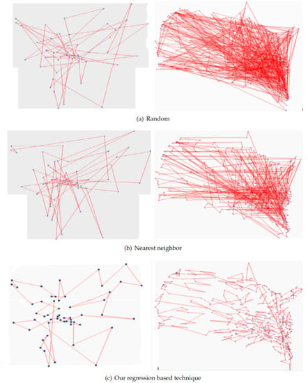
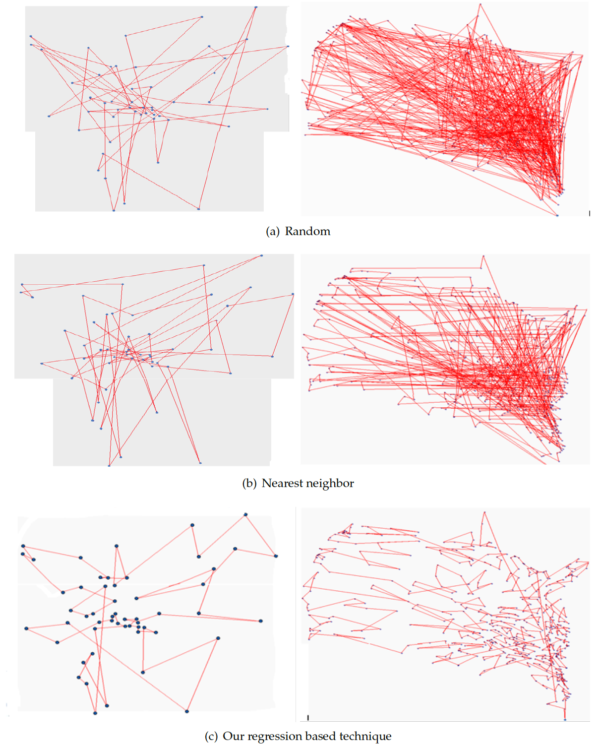
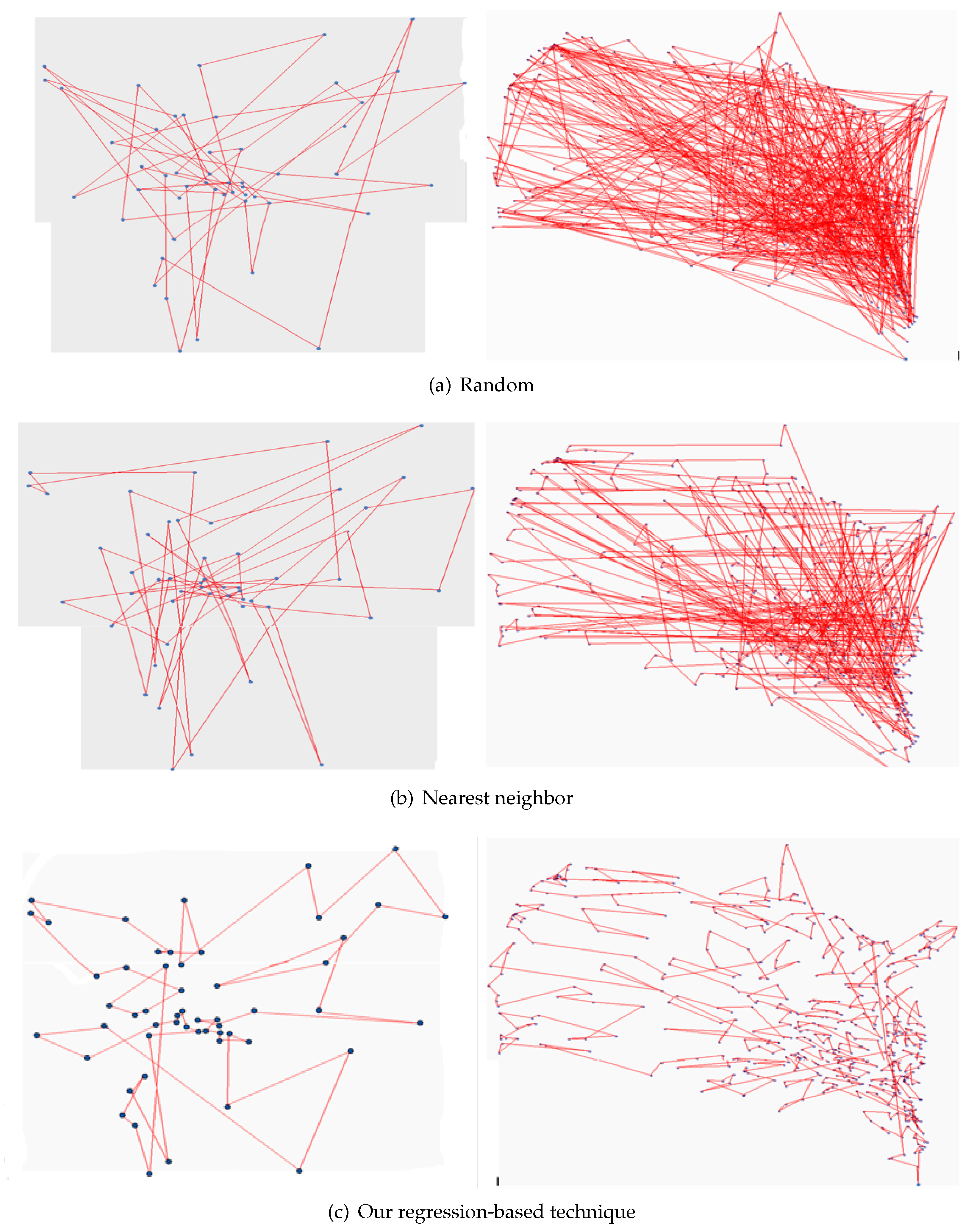
• Random Initialization: Random initial population seeding technique is the simplest and the most common technique that generates the initial population to GA. This technique is preferred when the prior information about the problem or the optimal solution is trivial. The sentence ‘generate an initial population’ related to the process of generating the initial population by using random initialization technique. In TSP, the random initialization technique selects the cities of the initial solutions randomly. During the individual generation, the random initialization technique generates a random number between 1 and n. If the current individual is already contains the generated number, then it generates a new number. Otherwise, the generated number is added to the current individuals. The Operation is repeated until the desired individual size (n) is reached. There are many random initial population methods aim to generate a random numbers such as the uniform random sequence, Sobol random, and quasi random [2,48].
• Nearest Neighbor: The nearest neighbor (NN) is considered as one of the most common initial population seeding technique. NN may still good alternative to random initial population technique in order to generate an initial population solutions that are used in solving TSP with GAs [49,50,51,52,53]. In the case of NN technique, the generation of each individual starts by selecting random city as the starting city and then the nearest city to be added as the new starting city. Iteratively, NN adds the nearest city to the current city that was not added to the individual until the individual includes all the cities in the problem space. The generated individuals from the NN population seeding can improve the evolving search process in the next generations as they were created from a city nearest to the current city [52].
• Selective Initialization: Yang [54] presented a selective initial population technique based on the K-nearest neighbor (KNN) sub graph. The KNN builds a graph contains all cities such as $c_i$ and $c_j$, based on the distance matrix. Where $c_i$ is one of the KNN cities of $c_j$ or $c_j$ is one of the KNN cities of $c_i$. The selective initial population technique grants the higher priority to the KNN sub graph edges. Firstly, from the city c, the next city will be randomly selected from c’s KNN list, but if all cities of c in KNN list are selected, then the next city is randomly selected from unvisited cities.
• Gene Bank: Wei et al. [55] proposed a greedy GA that depends on Gene Bank (GB) to generate the initial population to GA. GB technique aims to generate a high quality initial population solution. The GB is created based on the distance between cities by gathering the permutation of N cities. The initial population solutions that are generated from the GB are greater than the average fitness. In the case of solving TSP with N cities, the GB is constructed from c closer cities to city I, where c is the gene size less than or equal $n-1$. Each gene of the first city, I, is randomly chosen. Then, the closest unvisited city j from the i-th row is selected and from the j-th row the closest unvisited city k is selected. On the other hand, if all j-th row cities are visited, then the next city is randomly chosen from unvisited cities list.
• Sorted Population: Yugay et al. [28] proposed a sorted initial population technique to modify and improve GA based on the principle of the better offspring’s which are generated from the best parents. SP technique generates a large number of initial population solutions and sorts the min ascending order based on their fitness value in case of TSP-short distance. Finally, some of initial populations that have bad fitness are eliminated. The probability of finding a good solution in the population is very high when the initial population is very large. So, the sorted initial population technique is more likely to find a favorable initial population solution.
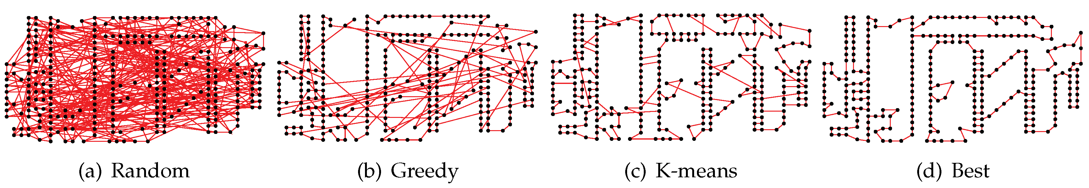
• K-means Initial Population: Deng et al. [33] introduced a new initial population technique to improve the performance of GA by using k-means algorithm for solving TSP. The proposed strategy used the k-means clustering to split a large-scale of TSP into small groups k, where $K=[\sqrt{N}+0.5]$ and N = number of cities. Next, KIP applies GA to find the local optimal path for each groups and a global optimal path that connects each local optimal solution, see Figure 6. K-means based initial population technique was compared with two initializations, random and gene bank initialization techniques. The results showed that this particular initialization technique is more efficient to improve GA.
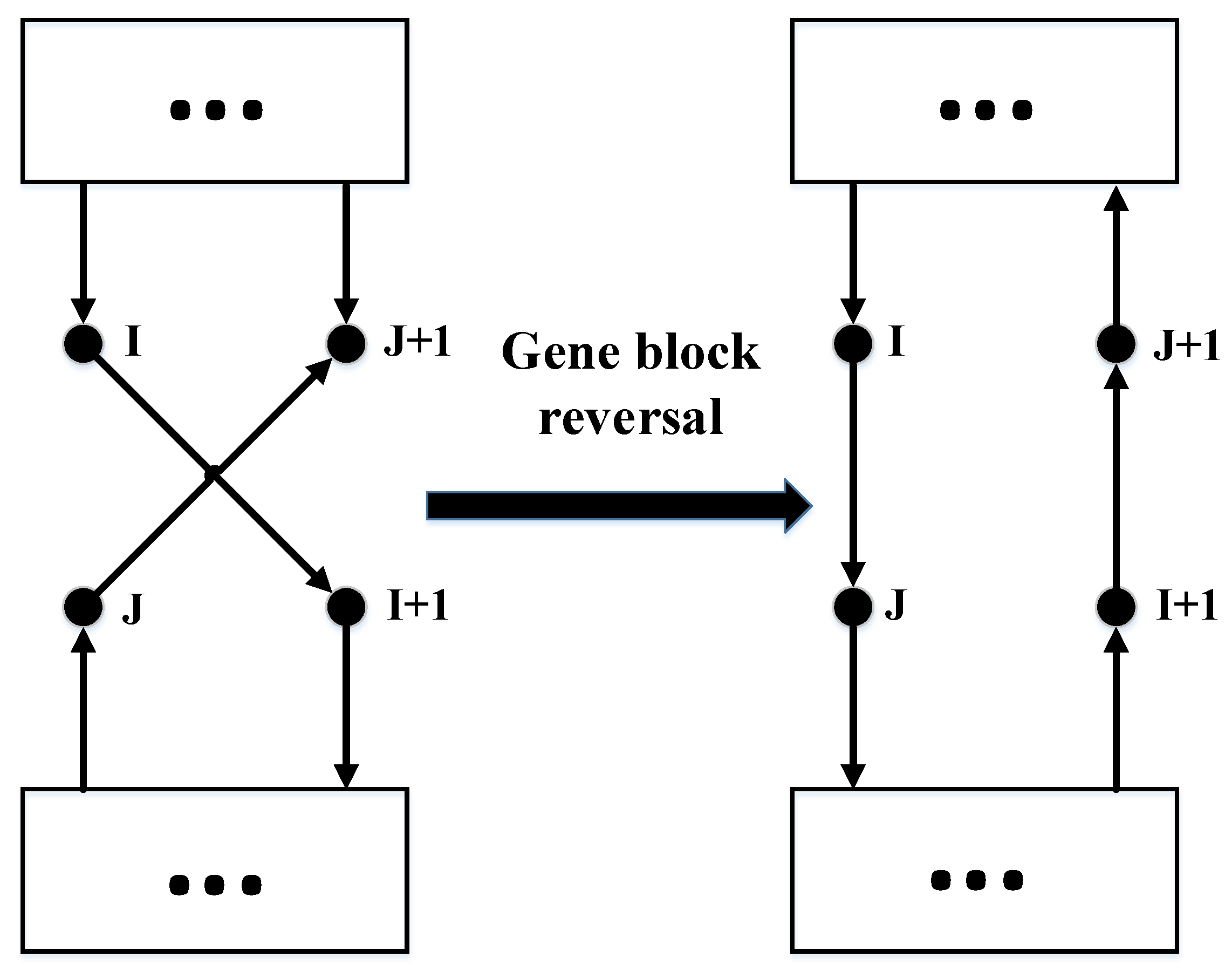
• Knowledge Based Initialization: Li et al. [56] proposed a knowledge based initialization technique to elevate the performance of GA in solving TSP. The main idea of KI based on generating initial population without path crossover, see Figure 7. However, when the number of involved nodes is large; it is too difficult to delete the crossover path without triggering another path. KI uses a heuristic method based on coordinate the transformation and the polar angle along with learned knowledge to create the initial population. The main idea is to split the plane into disjoint sectors; by increasing the polar angle to choose the cities that does not cause path crossover. Knowledge based initial population technique was compared to four other initializations: random, NN, gene bank, and Vari-begin with Vari-diversity techniques. The results showed that knowledge based nitialization technique is better than other techniques on the improvement of GA.
• Ordered Distance Vector Population Seeding: Paul et al. [7,57] disclosed an initial population seeding techniques that have a property of randomness and individual diversity based on the ordered distance vector (ODV). Three different initial population seeding techniques have been lunched based on ODV, namely ODV-EV, ODV-VE, and ODV-VV.
  The best adjacent (BA) number plays an important role in the individual diversity of the population. It assumes that any city $c_i$ in the optimal solution is connected to city $c_j$, where $c_j$ is one of nearest BA number of cities to $c_i$. In addition, Indevlen is the number represents the number of cities in each individual. In ODV techniques, the ordered distance matrix (ODM) size is created by using the value of BA and the given problem distance matrix. The techniques of generating the initial population using the ODM can be represented as follows:

  –

  ODV-EV. In ODV-EV technique, each individual in the populations begins with same city. A random number (BAi) is generated within the (BA) before inserting each city into each individual. The podv-ev that is generated using the ODV-EV technique can be represented as:

  $$\begin{array}{c}\hfill P_{ODV-EV}=\left[\begin{array}{ccccc}{\theta }_1\left(1\right)& {\theta }_1\left(c_2\right)& {\theta }_1\left(c_3\right)& \cdots & {\theta }_1\left(c_n\right)\\ {\theta }_2\left(1\right)& {\theta }_2\left(c_2\right)& {\theta }_2\left(c_3\right)& \cdots & {\theta }_2\left(c_n\right)\\ {\theta }_3\left(1\right)& {\theta }_3\left(c_2\right)& {\theta }_3\left(c_3\right)& \cdots & {\theta }_3\left(c_n\right)\\ \dots & \dots & \dots & \dots & ⋮\\ {\theta }_o\left(1\right)& {\theta }_o\left(c_2\right)& {\theta }_o\left(c_3\right)& \cdots & {\theta }_o\left(c_n\right)\end{array}\right]\end{array}$$

  (2)

  where $\theta$—an individual in the $P_{ODV-EV}$, o—individuals total number in the population $P_{ODV-EV}$, n—problem size. Each individual first city is remained same, i.e., ${\theta }_1\left(1\right)$ $={\theta }_2\left(1\right)$ $={\theta }_3\left(1\right)$ $\dots ={\theta }_o\left(1\right)$.

  –

  ODV-VE. In ODV-VE technique, each individual is assigned a random number (BAi) which is generated within the BA; and the same random number (BAi) is used to adjust each city in the individual. After that, the BA number of individuals, in the population begins with the same initial city number. The ODV-VE technique can be represented as:

  $$\begin{array}{c}\hfill P_{ODV-VE}=\left[\begin{array}{ccccc}{\theta }_1\left(1\right)& {\theta }_1\left(c_2\right)& {\theta }_1\left(c_3\right)& \cdots & {\theta }_1\left(c_n\right)\\ {\theta }_2\left(1\right)& {\theta }_2\left(c_2\right)& {\theta }_2\left(c_3\right)& \cdots & {\theta }_2\left(c_n\right)\\ \dots & \dots & \dots & \dots & ⋮\\ {\theta }_{ba}\left(1\right)& {\theta }_{ba}\left(c_2\right)& {\theta }_{ba}\left(c_3\right)& \cdots & {\theta }_{ba}\left(c_n\right)\\ {\theta }_1\left(2\right)& {\theta }_1\left(c_2\right)& {\theta }_1\left(c_3\right)& \cdots & {\theta }_1\left(c_n\right)\\ \dots & \dots & \dots & \dots & ⋮\\ {\theta }_{ba}\left(2\right)& {\theta }_{ba}\left(c_2\right)& {\theta }_{ba}\left(c_3\right)& \cdots & {\theta }_{ba}\left(c_n\right)\\ {\theta }_1\left(n\right)& {\theta }_1\left(c_2\right)& {\theta }_1\left(c_3\right)& \cdots & {\theta }_1\left(c_n\right)\\ \dots & \dots & \dots & \dots & ⋮\\ {\theta }_{ba}\left(n\right)& {\theta }_{ba}\left(c_2\right)& {\theta }_{ba}\left(c_3\right)& \cdots & {\theta }_{ba}\left(c_n\right)\end{array}\right]\end{array}$$

  (3)

  where (BA) is the number of individuals and the first city is the same, i.e., ${\theta }_1\left(1\right)$ $={\theta }_2\left(1\right)$ $\dots ={\theta }_{ba}\left(1\right)$, ${\theta }_1\left(2\right)$ $={\theta }_2\left(2\right)$ $\dots ={\theta }_{ba}\left(2\right)$, and so on.

  –

  ODV-VV. In ODV-VV technique, a new random number (BAi) between 1 and BA is generated before inserting any city to any individual. The starting city for each individual is randomly selected. The generated initial population seeding from ODV-VV is efficient and has good individual diversity. The ODV-VV technique can be represented as:

  $$\begin{array}{c}\hfill P_{ODV-EV}=\left[\begin{array}{ccccc}{\theta }_1\left(c_1\right)& {\theta }_1\left(c_2\right)& {\theta }_1\left(c_3\right)& \cdots & {\theta }_1\left(c_n\right)\\ {\theta }_2\left(c_1\right)& {\theta }_2\left(c_2\right)& {\theta }_2\left(c_3\right)& \cdots & {\theta }_2\left(c_n\right)\\ {\theta }_3\left(c_1\right)& {\theta }_3\left(c_2\right)& {\theta }_3\left(c_3\right)& \cdots & {\theta }_3\left(c_n\right)\\ \dots & \dots & \dots & \dots & ⋮\\ {\theta }_o\left(c_1\right)& {\theta }_o\left(c_2\right)& {\theta }_o\left(c_3\right)& \cdots & {\theta }_o\left(c_n\right)\end{array}\right]\end{array}$$

  (4)

• Insertion Population Seeding: The process of the insertion initial population seeding (In) technique starts with a partial path that contains several randomly selected cities. Then, iteratively inserts the nearest city to any city in the partial path. Finally, adds the edge to the lowest cost position at the path [58].
• Solomon Heuristic Seeding: Solomon Heuristic is a modification of the heuristic that was proposed for the vehicle routing problem with time windows by Solomon [59]. It starts with a partial path contains two cities that are randomly selected. Next, it calculates the inserting cost at any possible positions on the path for each city that is not inserted in the path. Finally, inserts the city into the path at the optimal position cost.

Among other techniques we mention the relevant ones and indicate the review works done in this direction next. Raja and Bhaskaran [60] proposed a new technique called population reduction (PR) in their study. Population reduction applies tournament selection after dividing the initial population into groups to select the best fit candidates. After that, the selected best fit individuals are entered to simple GA. This technique has been carried out on $0/1$ knapsack problem to study the impact of multi variables as follows:

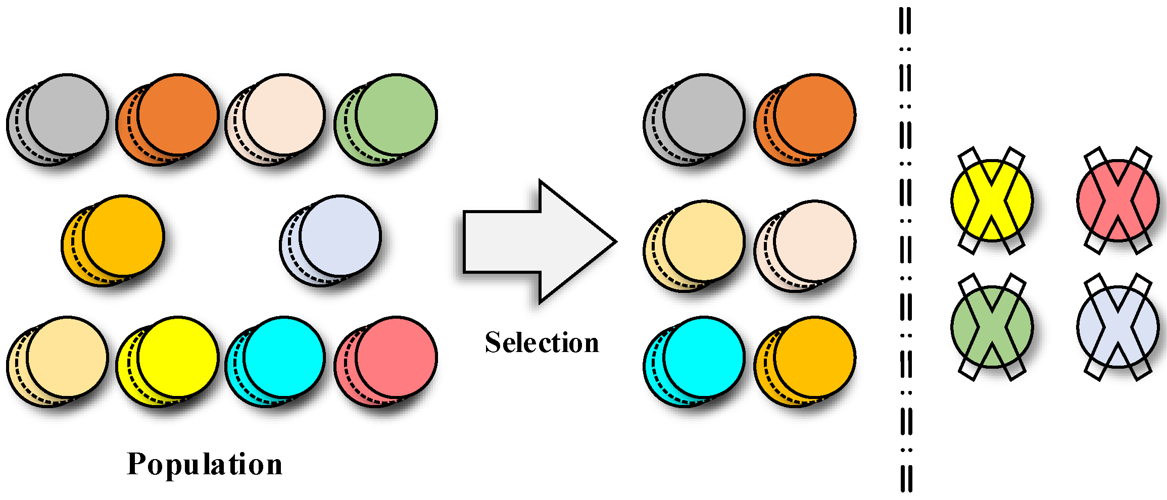
• Selection techniques such as Rank-based selection, Tournament selection, and Roulette Wheel selection.
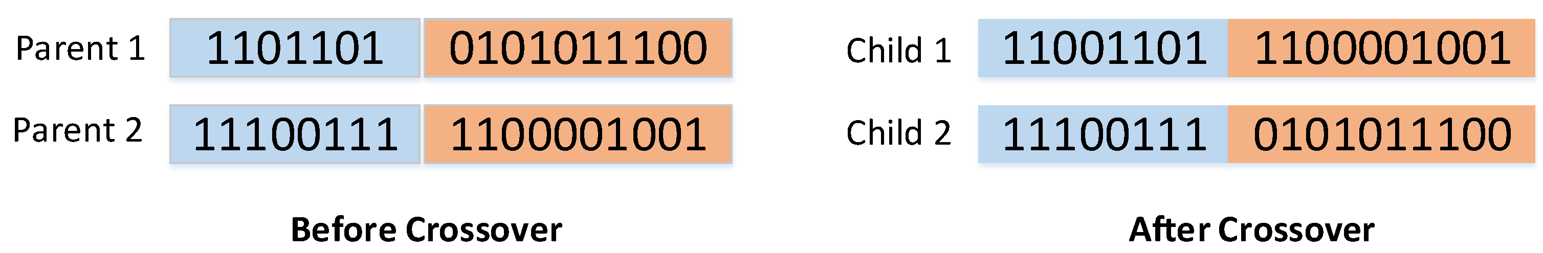
• Crossover: handled single-point crossover, two point crossover, and uniform crossover.
• Different Population Size.
• Crossover Rate: The rate of crossover operator used in each experiment.
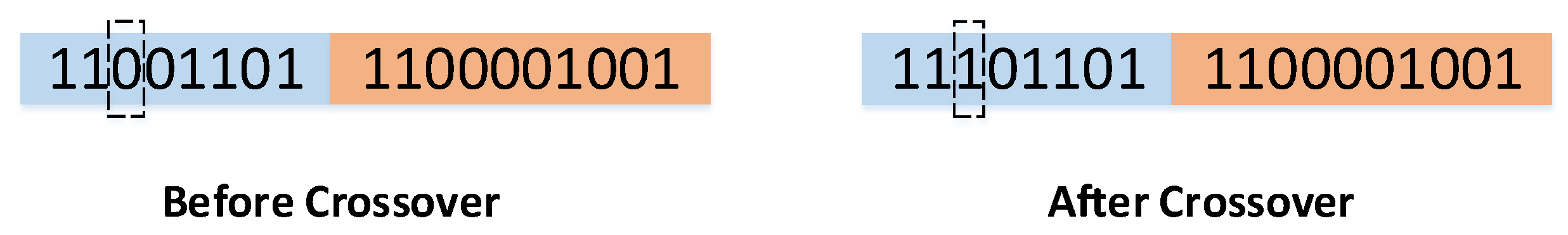
• Mutation Rate: Aims to find the best operator to their technique to be used in the experiments.

The experiment results when compared to simple GA depicted that the new methodology maintained less time than simple GA. Also, the result showed that tournament selection is the best performing selection techniques used along with PR.

Chiroma et al. [61] studied the appropriate values of critical variables that determine the fitness degree of the solution. They accomplished their work by developing a survey to discuss the impact of various variables by increase or decrease their proportion on solving problem using GA. The set of variables that have been involved in this study are the size of the population, mutation rate, and crossover rate. The findings are summarized up as follows:

• The larger population size, the higher efficiency in the search space.
• The moderate population size ranged from (12–4000).
• The increasing or decreasing of crossover rate leads to lose some solutions, where the range of crossover rate from ($0.1$–1) and the range of mutation rate from ($0.001$–1).

Shanmugam et al. [62] conducted a survey of different population seeding techniques that were carried out on TSP. They aimed to analyze the population seeding techniques performance, namely: random, NN, gene bank, selective initialization, and sorted population. They ordered the performance results of the previous population seeding techniques based on the factors of error rate (%) and convergence rate (%). The results showed that NN population technique is better than other investigated techniques. NN generates individuals with high fitness followed by selective initialization, and then gene bank techniques.

Paul et al. [63] conducted another survey using known population seeding techniques and a new population seeding technique namely: ODV based EV, VE and VV techniques. They studied, analyzed and carried out these techniques on traveling salesman problem. In addition to error rate and Convergence rate criteria that measure the population seeding techniques performance, new performance criteria were added such as computation time, convergence diversity, and average distinct solutions. The results showed that the ODV population seeding techniques have outperformed the other population seeding techniques for GA. ODV seeding techniques generate individuals with characteristics of high quality, diversity, and randomness. On the other hand, NN technique outperformed other techniques in terms of the average convergence and computation time criteria.

For studying the influence of applying heuristic initialization functions in GA, Osaba et al. [64] applied a combinatorial optimization problem using GA. Their experiments adopted three heuristic initialization functions: NN, Insertion (In) and Solomon heuristic. Several applications of GA have been designed to carry out the experiments in order to find the comparative model. Each version of applied GA has assigned a value of 100, 50, 10, and 0 called $G{A}_{\alpha }$, where $\alpha$ is the percentage of the population created by heuristic initialization functions. In their study, they used different initialization phase for each GA version. In addition, then, they measured the influence that has been emerged by each GA as a result of using heuristic functions. The results summarized that the NN technique has beaten other techniques in 13 cases out of 15 that means $86.66\%$ of the cases. Also, the GA50 version has had the best solution in $80\%$ of instances.

As it can be seen from the literature discussed above, there are some strong motivations to find better initial populations to start GA. It can be summarized as follows:

• Finding the best initial population is critical to find the optimal or near-optimal solution.
• The need of population diversity to avoid GA early convergence problem.
• Avoid falling in the local optimal solution problem:

  (a)

  Decrease the GA search time that are consumed for finding an optimal or near-optimal solution.

  (b)

  Decrease the numbers of generations that are needed to obtain the optimal or near-optimal solution.

The previous works indicate that there is still no consensus in using the initial population selection method. In this work, we propose a new method that is based on regression analysis to generate better initial populations for GA.

3. Proposed Initialization Technique Based on Linear Regression

Seeding the initial population is the first phase of the application of GAs. Random generation method of initial population is the most widely used method. It is considered as one of the most important GAs parameter that improves the GA performance to find the optimal solution. Indeed, enhancing GAs performance is achieved by increasing the speed of finding solution, improving individual diversity, and quality. Here, we develop a new population seeding technique using regression and successive partitioning of the main problem into sub-problems for GA. Our proposed method is tested on traveling salesman problem (TSP). The proposed technique depends on the linear regression technique and uses perpendicular lines that cross the regression lines at the center points.

Recall that the linear regression is a statistical approach to reveal the relationship between dependent variable and one or more independent variables. Linear regression correlates and models the relationship between two-dimensional sample points with two variables by fitting a linear equation [55]. The first variable is called explanatory variable or independent variable denoted by x, and the second variable is called a scalar dependent variable denoted y [28,65]. In linear regression, linear predictor functions are used to model the relationships with estimated parameters from the data [55,65]. The Linear regression equation has the form $y=a+bx$, where x is explanatory or independent variable and y is the dependent variable. While the constant a is the y-intercept and b is the slope of the line [66].

$$\begin{array}{c}\hfill a=\frac{\sum y\sum x^2-\sum x\sum xy}{n\sum x^2-{(\sum x)}^2},b=\frac{n\sum xy-\sum x\sum y}{n\sum x^2-{(\sum x)}^2}.\end{array}$$

(5)

Our proposed approach is based on the computation of regression lines, and the perpendicular lines that crosses the regression lines at the center points to divide a large-scale TSP problem to small sub-problems. The resulting sub-problems are repeatedly classified to fit into four categories to obtain local optimal solutions. Thus, the main procedures of the proposed method are:

(1)

start with dividing the large-scale TSP into four small sub-problems using regression line and the perpendicular line, and classify the points into four categories. Each category is divided into four new categories recursively by using the regression line and the perpendicular line. The process carries on until having the target category that contains a small number of instances (x,y) points. Maximum four cities or (x,y) points assigned to each category that are considered as initial population for TSP sub-problem. The process ends up when the local optimal solution is obtained for each category.

(2)

Rebuild the initial populations seeding by reconnecting all local optimal solutions together. Finally, mutate the initial population N times to obtain N solutions, where N is the population size.

In what follows, we utilize two of TSP cities berlin52, and att532 to illustrate the regression-based technique for initialization of GA, see Figure 8 that show these cities in $x-y$ scatter plots representation.

The following steps illustrate the new initialization technique designed to improve the GA for solving the well-known TSP:

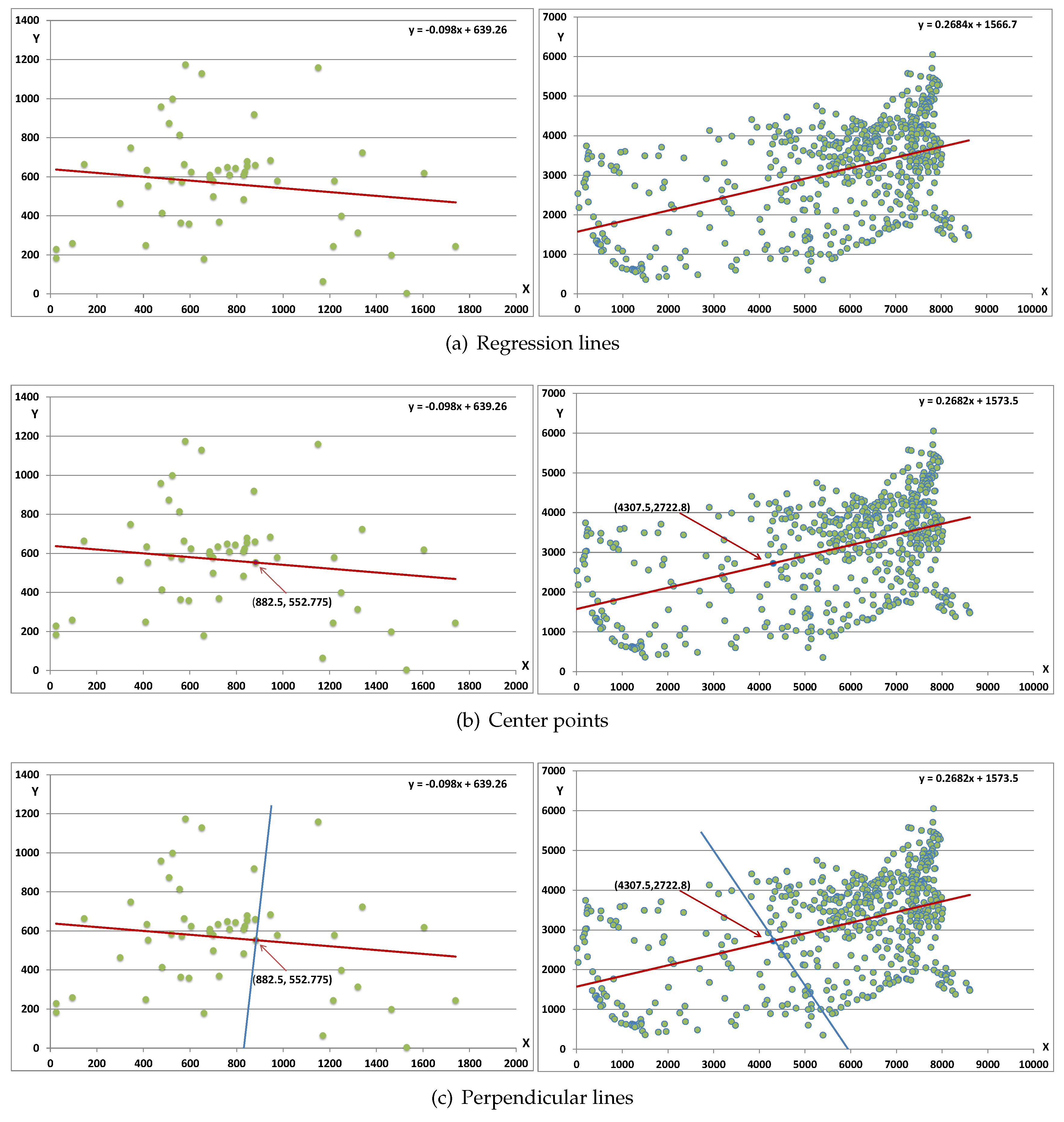
• Step 1: Find the regression line equation ($y=a+bx$) that divide the points into two sections. To compute the regression line for berlin52 ($N=52$ cities), we note that $\sum x=39440$, $\sum y=29375$, $\sum xy=21516075$, $\sum x^2=37704250$, so that we see the constants $a=639.2585$ the y-intercept, $b=-0.09803$ the slope of the line, see Equation (5). Thus, the regression line equation is given by $y=639.26-0.098x$. Similarly for att532 ($N=532$ cities), we note that $\sum x=3005687$, $\sum y=1640278$, $\sum xy=9983426703$, $\sum x^2=19649653721$, so that we see the constants $a=1566.5$ the y-intercept, $b=0.2684$ the slope of the line. Thus, the regression line equation is given by $y=1573.5+0.2682x$. See Figure 9a that shows these regression lines graphically.
• Step 2: Find the center points (x,y) of the regression lines. For berlin52 the center point ($882.5$, $552.775$) is calculated from the end points (25, $636.81$), (1740, $468.74$), for and att532 the center point ($4307.5$, $2722.8$) is calculated from the end points (8605, $3876.28$), (10, $1569.38$). See Figure 9b that shows these center points.
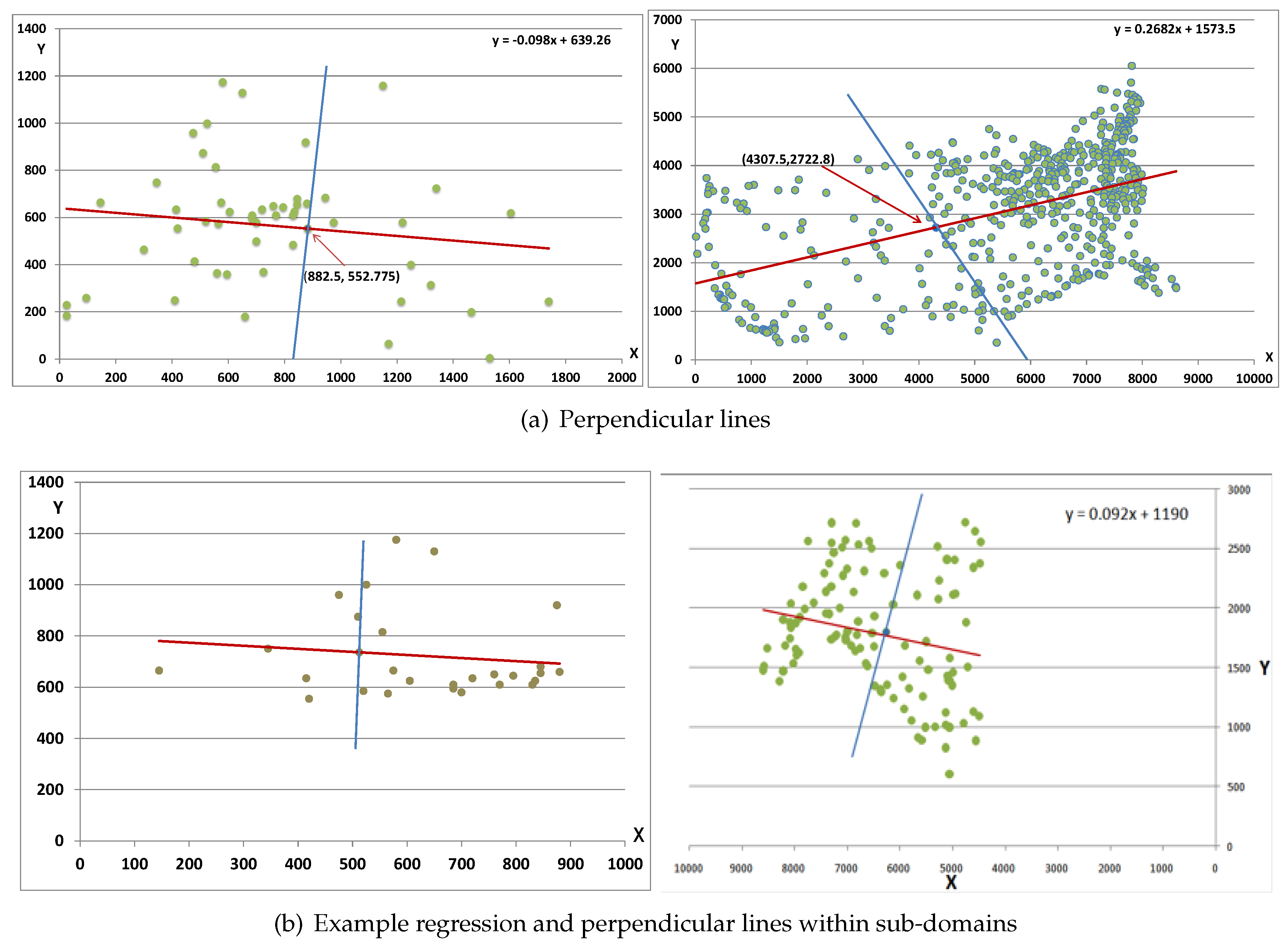
• Step 3: Find the perpendicular line equation that intersects the regression line at the center point. Note that the regression line slope is b, then the perpendicular line slope $-1/b$. The perpendicular line equation can then be obtained by using the line slope and the intersection point with the regression line (center point). See Figure 9c that shows these perpendicular lines.
• Step 4: Shift the center point to the origin point, and then allocate the regression line and the perpendicular line on the (x, y) axis. Next, classify the points into four categories A, B, C, and D, see Figure 10a.
• Step 5: Recursively, compute the regression and perpendicular lines (Steps 1 to 4) four times for each category A, B, C, and D, see Figure 10b for examples.
• Step 6: Terminate the recursive computation if the number of points (cities) less than or equal to four.
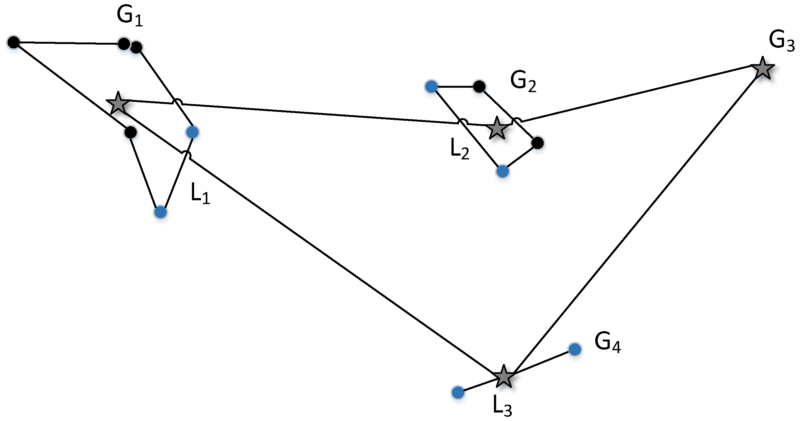
• Step 7: Select a random city to be the starting city, and then add the nearest city as new starting city until having all cities connected in the category of the local path. The group in each category is connected with the nearest group in other categories until all groups are connected in a global path.

In summary, Assuming that a TSP can provide the location information about its cities, it is possible to repeatedly cluster these cities using the regression line that divides these cities equally based on their y-coordinates, finding the perpendicular line passing the center of the regression line will further divide these cities based on their x-coordinates, this gives four sub-TSPs, each of these groups has several adjacent or neighboring cities. The algorithm recursively repeats the same process four times on the four sub problems to go deeper until the size of the sub problem becomes very small, in this work we choose the number 4 or less as the stopping criteria of the recursive algorithm. Since the algorithm uses the regression line, it guarantees that the small number of cities that it ends with are more likely to be neighbors and closer to each others from the other cities, and therefore, connecting them with each others is better than connecting any of them with further cities, as these local links are minimized, and minimizing the local links attributes in finding a smaller global route. However, there is a problem of connecting which city from a sub problem with which city from another sub problem, this problem remains unsolved in this work, as we think that the GA will take care of this problem by evolving new solutions. The previous algorithm provides only one solution, which is the initial seed of the initial population, since the population needs more than one solution to start the GA, we used this seed solution to derive n solutions using the mutation operator, which is used $n-1$ times to mutate the seed solution, where n is the size of the population. We used the mutation operator here and not the crossover operator to increase the diversity of the initial population. When the initial population is completed, The GA will follow up to optimize for the solutions. Figure 11 shows a comparison population initialization of the obtained by our proposed regression-based technique with random, nearest neighbor based ones on berlin52, and att532.

4. Experimental Results and Discussion

In addition to the proposed seeding technique, we present experimental results and performance analysis of two different population seeding approaches, namely the random initialization, which is used by most GAs [2,48], and the nearest neighbor (NN) approach. The NN approach used here is similar to that of [49,50,51,52,53], but not exactly the same, as we implemented the general NN approach and compared with our own implementation rather than comparing with each specific NN method. The general NN approach used for our comparison is based on selecting a current city randomly, then linking the nearest city to the current city and carry on until linking all cities to form the final rout. All the experiments have been carried out in the same test setup to generate individuals for evaluation purpose using specific performance factors.

Table 1. GA configuration parameters for experiments.

No	Parameter	Value/Technique
1	Population Size	100
2	Generation Limit	3000
3	Initialization Technique	Random, NN, and regression
4	Crossover Method	one-point modified crossover
5	Crossover Probability	0.82
6	Mutation Method	Exchange mutation
7	Mutation Probability	0.1
8	Selection	Roulette wheel
9	Termination Condition	Generation limit

displays the GA parameters that have been chosen to conduct our experiments here. Roulette wheel selection strategy was used to assign fitness to each individual. This is a traditional process to assign the fitness function to each individual (chromosome) in the population. The best solution is measured by fitness level that links the probability of selection with each chromosome [67].

Our experiments used one-point modified crossover and exchange mutation approaches. The single-point modified crossover strategy identifies the point in the chromosomes randomly, and then, switches genes after this point between the individuals to produce new children [68]. The exchange mutation strategy is based on the random selection of two genes and the switching between their positions [69]. Each technique was applied 20 times, and the average of all executions results was used for the purposes of experimental analysis.

4.1. Experimental Setup

All the experiments were carried out in a similar environment setting for all initialization techniques to make a fair assessment. The results help to assess the performance and efficiency of the regression-based technique for GA’s population initialization in comparing with the performance of different initialization techniques. All initialization techniques under investigation used the problem examples of traveling salesman problem. The Experiments were implemented using Microsoft Visual Studio 2008 tool with TSP benchmark datasets obtained from TSPLIB (https://www.iwr.uni-heidelberg.de/groups/comopt/software/TSPLIB95/). The selected TSP examples for experimentation were classified into four classes based on their problem size, see

Table 2. Different sized TSP problems.

No	Class	Instance Size	Instances
1	Class 1	Size ≤ 100	KroA100, pr76, eil51
2	Class 2	100 < Size ≤ 500	KroA200, pr144, lin318
3	Class 3	500 < Size ≤ 1000	att532, rat783, u724
4	Class 4	1000 < Size ≤ 5000	fl1577, fnl4461, d2103

, which displays the classes and the TSP instances that belong to.

4.2. Assessment Criteria

The performance factors that have been identified as measurements should be considered in investigating various initialization techniques namely, error rate, average convergence and final solution error:

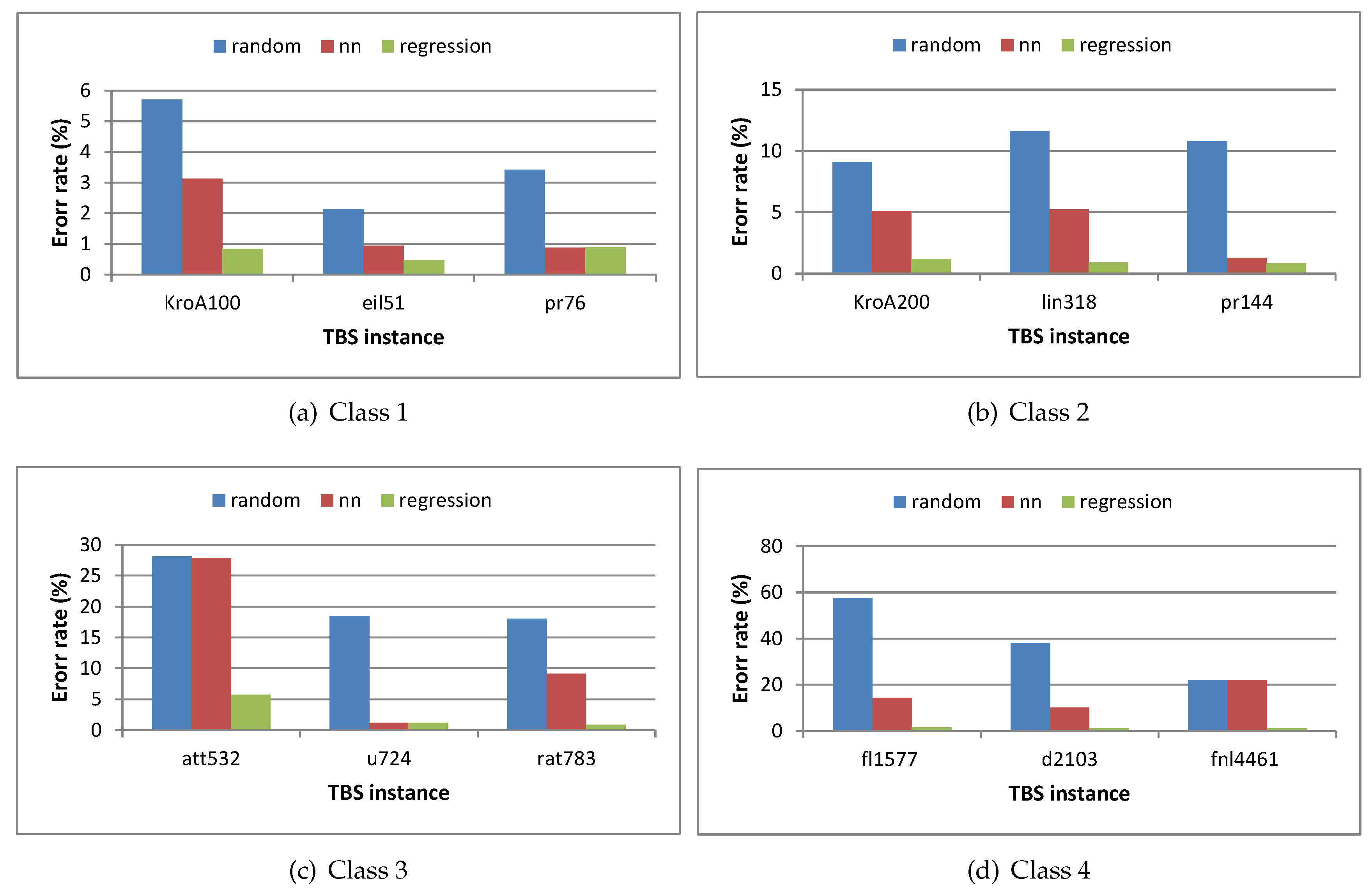
• Error Rate is the percentage of the difference between the known optimal solution and the fitness value of the solution for the problem [52,70,71]. It can be represented as:

  $$\begin{array}{c}\hfill \mathrm{Error}\mathrm{Rate}(\%)=\frac{\mathrm{Fitness}-\mathrm{Optimal}\mathrm{fitness}}{\mathrm{Optimal}\mathrm{fitness}}\times 100\end{array}$$

  (6)
  The error rate can be classified into two types based on the fitness values in the population. First, individuals with high error rate due to the initial population with worst fitness value. Second, individuals with low error rate due to the initial population with worst fitness [32].
• Average Convergence is the convergence rate of solutions in the initial population [26,32]. It can be defined as:

  $$\begin{array}{c}\hfill \mathrm{Average}\mathrm{Convergence}(\%)=1-\frac{\mathrm{Average}\mathrm{fitness}-\mathrm{Optimal}\mathrm{fitness}}{\mathrm{Optimal}\mathrm{fitness}}\times 100\end{array}$$

  (7)

  where, average fitness is the fitness value average in the population, and the optimal fitness is the recognized optimal value of identical instance.
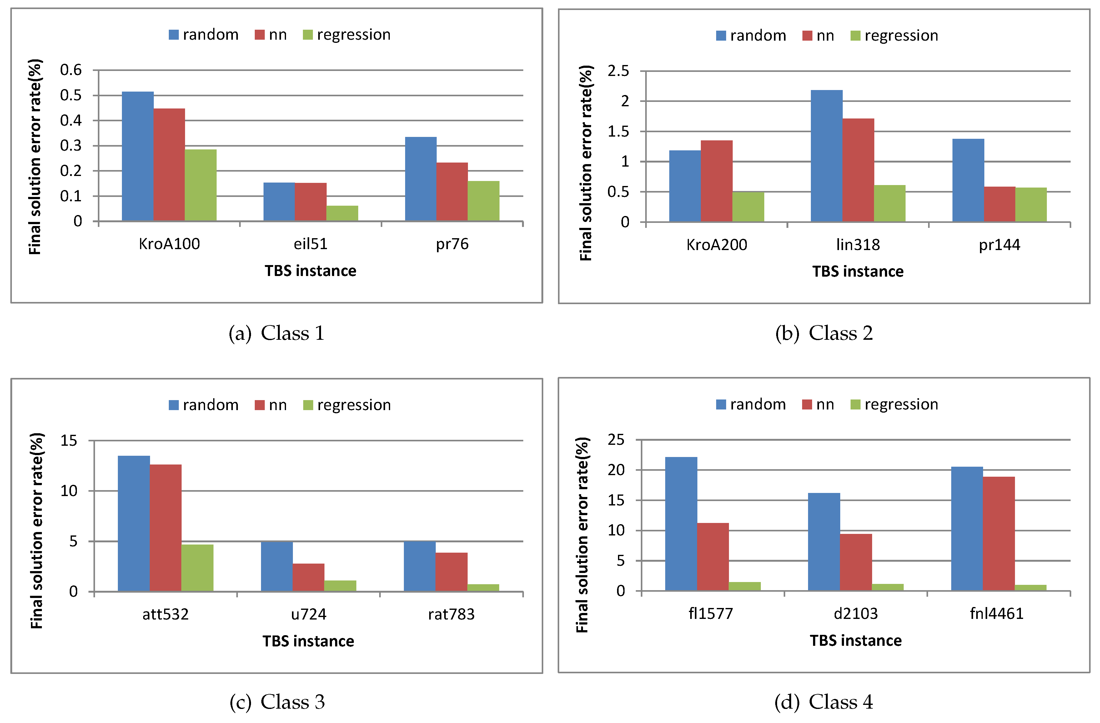
• Final Solution Error Rate refers to the difference between the known optimal solution and the final solution that is resulted when applying the GAs on TSP instances using one of initial population technique. It can be represented as:

  $$\begin{array}{c}\hfill \mathrm{Final}\mathrm{Solution}\mathrm{Error}\mathrm{Rate}(\%)=\frac{\mathrm{Final}\mathrm{solution}-\mathrm{Optimal}\mathrm{fitness}}{\mathrm{Optimal}\mathrm{fitness}}\times 100\end{array}$$

  (8)
  This factor measures the quality of the generated population by finding the effect of applying initial population technique on Gas performance to obtain a solution near to optimal one.

Further, we use the following statistical tools to measure performance of different initialization techniques:

• ANOVA: A one-way analysis of variance (ANOVA) is used as one of statistical analysis techniques that test if one or more groups mean are significantly different from each other. Specifically, the ANOVA statistical analysis tests the null hypothesis:

  $$H0:{\mu }_1={\mu }_1={\mu }_1=\dots ={\mu }_k$$

  where, ${\mu }_1$ = group mean and k = the number of groups. The one-way ANOVA test is performed with critical value $\alpha$ (the value that must be exceeded to reject the null hypothesis (H0)). H0 is accepted if the sig value is greater than the critical value ($\alpha$) which equals ($0.05$) in this work. Otherwise, the H0 should be rejected and H1 should be accepted. That means there are two groups at least are different from each other. The one-way ANOVA cannot determine which specific groups were statistically different from each other. Therefore, to determine the different groups, a post hoc test such Duncan’s multiple range test, and least significant difference (LSD) test are used.
• Duncan’s multiple range test (DMRT): This is considered as one of the most important statistical analysis tests that is used to find group differences after rejecting the null hypothesis. It is called post hoc or multiple comparison tests [72]. The Duncan’s multiple range tests compares all pairs of groups mean. It computes the numeric boundaries that allow classifying the difference between any two techniques range [73]. If there is a significant difference between the population means, DMRT will have a high probability of declaring the difference. For this reasons, the Duncan’s test has being the most popular test among researchers. The DMRT was implemented in this work for classifying the study groups (random, nearest neighbor, and regression) into homogenous group. The classified groups and sig value show if there is a significant difference between groups or not. Pairs of means resulting from a group comparison study with more than two groups are significantly different from each other with $5\%$ level of significance ($\alpha$). However, DMRT produces information about the significant difference between groups without differentiates their mean.
• Least significant difference (LSD): This is one of post-hoc test developed by Ronald Fisher in 1935. In general, the (LSD) is a method used to calculate and compare groups mean after rejecting the ANOVA null hypothesis (H0) of equal means using the ANOVA F-test [72]. Rejecting H0 means there are at least two means different from each other, but if the ANOVA F-test fails to reject the H0, there will be no need to apply LSD as it will incorrectly propose a significant differences between groups mean. LSD computes the minimum significant variance between two means, and to declare any significant difference larger than the LSD.

4.3. Experimental Results and Discussion

In this section, the efficiency of GA is discussed in the case of using Random, NN, and our proposed regression-based technique for GAs population initialization in solving TSP instances under similar experimental environment.

The error rate results show that the regression-based technique for GAs maintains the minimum error rate than other seeding techniques Random and NN. Also, it is clear that NN error rate $9.2\%$ is less than Random technique of $18.6\%$. This clarifies that the generated individuals by our proposed regression-based technique for GAs are better fit the quality measures than the individuals generated by NN and Random techniques. This difference referred to the mechanism of our new technique that divides the problem into small sub problems.

Table 3. Experimental results with respect to the Error Rate (%) for different population seeding techniques.

Si/no	Class	Problem	Optimal Solution	Random			NN			Regression
				Best	Worst	Time	Best	Worst	Time	Best	Worst	Time
1	Class 1	KroA100	21282	5.707593	6.1524763	2	3.119679	6.0301663	3	0.834367	0.930646	33
2		eil51	426	2.129108	2.4389671	1	0.943662	1.1197183	1	0.467136	0.615023	20
3		pr76	108159	3.412661	3.7008293	1	0.873483	1.0330994	2	0.881794	1.043667	29
4	Class 2	KroA200	29368	9.112061	9.7429856	5	5.112435	5.259398	3	1.190207	1.318646	66
5		lin318	42029	11.64106	12.197197	6	5.216184	5.6842656	5	0.916153	0.958077	115
6		pr144	58537	10.81328	11.651656	3	1.265268	1.5631652	2	0.848421	0.90172	56
7	Class 3	att532	27686	28.14841	54.836199	17	27.91581	54.879	12	5.753486	6.145778	292
8		u724	41910	18.48289	19.108304	20	1.159127	19.011644	19	1.159127	1.2157	217
9		rat783	8806	18.01306	18.654781	21	9.135703	9.4115376	23	0.872473	0.90427	230
10	Class 4	fl1577	22249	57.4638	58.642726	56	14.26936	58.611398	66	1.532114	1.587802	483
11		d2103	80450	38.15525	38.674779	5	10.16072	38.595165	100	1.162884	1.202722	642
12		fnl4461	182566	22.101	43.99948	6	22.06794	43.880471	408	1.018339	1.03906	1516

shows the experimental results of the initial population techniques with respect to error rate for the best individuals and the worst individuals in the initial population for each technique.

Figure 12 illustrates the error rate that attained by different initial population techniques for several classes of problem example. Analysis of Variance test (ANOVA) test determines the significance of means difference between two or more independent groups. In this study, the one-way ANOVA analysis was used to determine if the different techniques have significant differences or not. ANOVA, Duncan, and LSD were applied to examine the existence of significant difference between the different techniques. Findings show different levels of error rate prevailed among Random, NN and our Regression techniques.

Table 4. Descriptive analysis of random, NN and our Regression technique with respect to error rate.

	N	Mean	Standard Deviation	Std. Error	95% Confidence Interval for Mean		Minimum	Maximum
					Lower Bound	Upper Bound
Random	12	18.7650	16.13439	4.65760	8.5137	29.0163	2.13	57.46
NN	12	8.4366	8.89413	2.56751	2.7856	14.0877	0.87	27.92
Regression	12	1.3864	1.39959	0.40403	0.4971	2.2756	0.47	5.75
Total	36	9.5293	12.63646	2.10608	5.2538	13.8049	0.47	57.46

shows that regression technique has the minimum error rate compared to Random and NN techniques. Also, NN mean is much less than Random method.

Table 5. ANOVA analysis of Random, NN and our Regression with respect to error rate.

	Sum of Squares	df	Mean Square	F	Sig.
Between Groups	1833.595	2	916.798	8.057	0.001
Within Groups	3755.212	33	113.794
Total	5588.807	35

shows ANOVA test result that proves a significant difference in mean values with respect to error rate of adopted techniques, Random, NN and our regression. The sig value $0.001$, as observed, there is a significant difference between the groups. To find the group differences, a multiple comparisons tests have been carried out such as Duncan and LSD.

Duncan results in

Table 6. Duncan: Homogonous Error rate subset.

Technique	N	Subset for $\mathit{\alpha }=0.05$
		1	2
Random	12		18.7650
NN	12	8.4366
Regression	12	1.3864
Sig.		0.115	1.000

show that there are two homogeneous groups exist when applying the different population initialization techniques in respect to their error rate.

Table 7. Multiple Comparisons (Random, NN and our Regression) significant with respect to the Error Rate. * The mean difference is significant at the $0.05$ level.

Technique	Technique	Mean Difference	Std. Error	Sig.	95% Confidence Interval
(I)	(J)	(I–J)			Lower Bound	Upper Bound
Random	NN	10.32840 *	4.35496	0.024	1.4682	19.1886
	Regression	17.37864 *	4.35496	0.000	8.5184	26.2389
NN	Random	−10.32840 *	4.35496	0.024	−19.1886	−1.4682
	Regression	7.05024	4.35496	0.115	−1.8100	15.9105
Regression	Random	−17.37864 *	4.35496	0.000	−26.2389	−8.5184
	NN	−7.05024	4.35496	0.115	−15.9105	1.8100

shows that there is a significant mean difference between Random and NN techniques (sig = $0.24$) as well as a significant difference between Random and our Regression techniques (sig = $0.000$). Also, a significant difference between NN and our Regression (sig = $0.024$) as can observed from Table 7 our Regression technique has the minimum error rate with significant difference in pair wise comparisons with Random and NN due to the Individuals that generate using regression technique is better than Individuals that generate from other technique based on their Working mechanism.

The average convergence results show that the regression-based technique for GA’s population initialization achieved average convergence rate of $98.9\%$ greater than other seeding techniques. The regression-based technique performs better, particularly with the large size problems. Also, results show that NN average convergence is greater than Random. These results mean that the individuals who are generated by regression-based technique is the nearest to the optimal value that has average convergence close to $98.9$.

Table 8. Average convergence (%) rate results for Random, NN and our regression-based techniques.

Si/no	Class	Problem	Optimal Solution	Population Seeding Techniques
				Random	NN	Regression
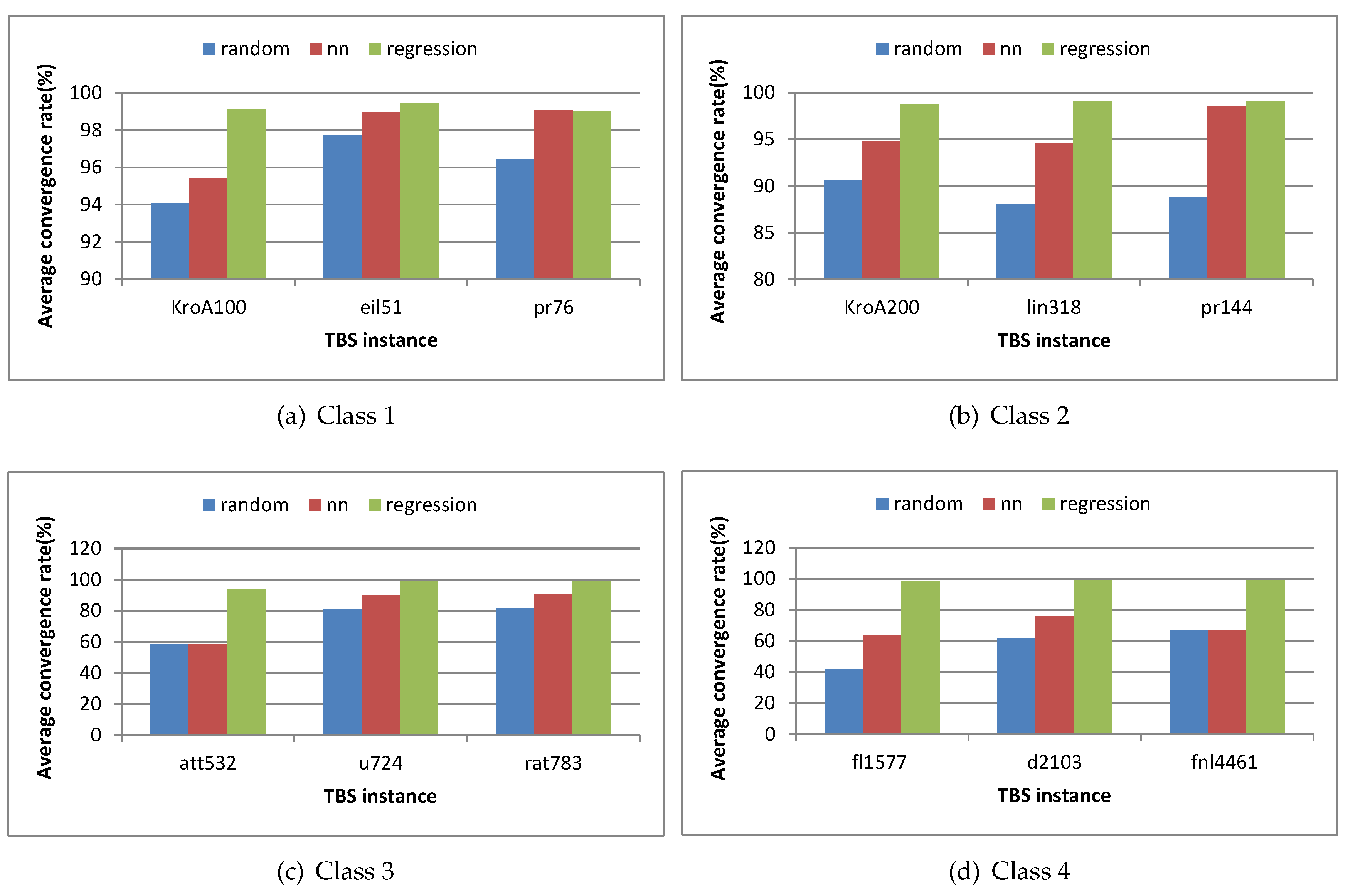
1	Class 1	KroA100	21282	94.0699652	95.425078	99.117494
2		eil51	426	97.7159624	98.96831	99.45892
3		pr76	108159	96.4432548	99.046709	99.037269
4	Class 2	KroA200	29368	90.5724768	94.814083	98.745573
5		lin318	42029	88.0808727	94.549775	99.062885
6		pr144	58537	88.7675316	98.585783	99.12493
7	Class 3	att532	27686	58.5076934	58.602597	94.050368
8		u724	41910	81.2044023	89.914615	98.812586
9		rat783	8806	81.6660799	90.72638	99.111628
10	Class 4	fl1577	22249	41.9467392	63.559621	98.440042
11		d2103	80450	61.5849845	75.622057	98.817197
12		fnl4461	182566	66.9497579	67.025796	98.971301

shows the experimental results of the initial population techniques with respect to average convergence (%). The average convergence (%) obtained for the GA using a various initial population techniques is shown in Figure 13.

Results in

Table 9. Descriptive analysis of Random, NN and our Regression technique with respect to average convergence.

Technique	N	Mean	Standard Deviation	Standard Error	95% Confidence Interval for Mean		Min.	Max.
					Lower Bound	Upper Bound
Random	12	78.9591	17.70148	5.10998	67.7122	90.2061	41.95	97.72
NN	12	85.5701	15.05677	4.34652	76.0035	95.1367	58.60	99.05
Regression	12	98.5625	1.44309	0.41658	97.6456	99.4794	94.05	99.46
Total	36	87.6972	15.44635	2.57439	82.4709	92.9235	41.95	99.46

show that our Regression technique has the maximum average convergence (Mean = 98.5) compared to Random and NN techniques (Mean = $85.57$). Also, NN mean is slightly greater than Random method (Mean = $78.95$). ANOVA test results show whether one or more group means are significantly different according to average convergence. The One- way-ANOVA test, which was used, helps to determine if the different techniques under investigation have significant differences or not. ANOVA, Duncan and LSD were applied to explore the significant difference between the different techniques.

Table 10. ANOVA analysis of Random, NN and our Regression with respect to average convergence.

Sum of Squares	df	Mean Square	F	Sig.
Between Groups	2387.201	2	1193.601	6.605	0.004
Within Groups	5963.442	33	180.710
Total	8350.643	35

shows ANOVA test results that prove a significant difference in mean values with respect to average convergence of adopted techniques, Random, NN and our Regression. The sig value ($0.004$), as observed, means that there is a significant difference between groups. To find the group differences, a multiple comparisons tests have been applied, Duncan and LSD.

Duncan results,

Table 11. Duncan: Homogonous average convergencesubset.

Technique	N	Subset for $\mathit{\alpha }=0.05$
		1	2
Random	12	78.9591
NN	12	85.5701
Regression	12		98.5625
Sig.		0.237	1.000

show that there are two homogeneous groups exist when applying the different population initialization techniques in respect to average convergence.

Table 12. LSD: Multiple Comparisons (Random, NN and our Regression) significant w.r.t average convergence. * The mean difference is significant at the $0.05$ level.

Technique	Technique	Mean Difference	Standard	Sig.	95% Confidence Interval
(I)	(J)	(I–J)	Error		Lower Bound	Upper Bound
Random	NN	−6.61092	5.48802	0.237	−17.7764	4.5545
	Regression	−19.60337 *	5.48802	0.001	−30.7688	−8.4379
NN	Random	6.61092	5.48802	0.237	−4.5545	17.7764
	Regression	−12.99245 *	5.48802	0.024	−24.1579	−1.8270
Regression	Random	19.60337 *	5.48802	0.001	8.4379	30.7688
	NN	12.99245 *	5.48802	0.024	1.8270	24.1579

shows that there is insignificant mean difference between Random and NN techniques (sig = $0.23$) as well as a significant difference between Random and Regression techniques (sig = $0.001$). Also, a significant difference between NN and Regression (Sig = $0.024$). As can be observed from Table 12, regression technique has the maximum average convergence rate with significant difference in pair wise comparisons with Random and NN.

The final solutions error rate results show that the regression-based technique for GAs population initialization maintains the minimum error rate than other seeding techniques Random and NN. Also, results show that the NN technique error rate is lesser than Random technique. This demonstrates that the individuals generated by regression-based technique have better fit quality than those individuals who are generated by NN and Random techniques. Also, as we can see in

Table 13. Final solution error rate (%) results for Random, NN and our Regression techniques.

Si/no	Class	Problem	Optimal Solution	Population Seeding Techniques
				Random	NN	Regression
1	Class 1	KroA100	21282	0.514533409	0.447488488	0.28387839
2		eil51	426	0.153051643	0.151760563	0.06220657
3		pr76	108159	0.334713246	0.232944092	0.15975739
4	Class 2	KroA200	29368	1.183575661	1.349473917	0.48822868
5		lin318	42029	2.184444074	1.712403341	0.61007043
6		pr144	58537	1.376344876	0.585363958	0.57191264
7	Class 3	att532	27686	13.47315972	12.60865419	4.67371415
8		u724	41910	4.942157003	2.795419948	1.12181937
9		rat783	8806	4.982392687	3.87176357	0.74465705
10	Class 4	fl1577	22249	22.10749022	11.21874017	1.46520743
11		d2103	80450	16.16575637	9.38666128	1.14121193
12		fnl4461	182566	20.54833978	18.85593922	1.01935355

, the problem size has no significant impact on regression-based technique performance comparing to other seeding techniques Random and NN. This referred to the mechanism of our new technique that divides the problem into small sub problems.

Figure 14 illustrates the final solution error rate that attained by different initial population techniques for various classes of problem instances.

Results in

Table 14. Descriptive analysis of Random, NN and Regression technique with respect to final solution.

Technique	N	Mean	Standard Deviation	Standard Error	95% Confidence Interval for Mean		Min.	Max.
					Lower Bound	Upper Bound
Random	12	7.3305	8.34874	2.41007	2.0260	12.6350	0.15	22.11
NN	12	0.9808	1.23616	0.35685	0.1954	1.7663	0.06	4.67
Regression	12	0.1791	0.28387	0.08194	−0.0012	0.3595	0.02	1.02
Total	36	2.8302	5.73914	0.95652	0.8883	4.7720	0.02	22.11

shows that regression technique has the minimum difference average between optimal and final solution (Mean = $0.17$) compared to Random and NN techniques (Mean = $7.33$). Also, NN mean is greater than Random method (Mean = $0.98$). ANOVA test results show whether one or more group means are significantly different according to final solution differences. One-way-ANOVA test was used in order to determine if the different techniques under investigation have significant differences or not. ANOVA, Duncan and LSD were applied to explore the significant difference between the different techniques.

Table 15. ANOVA analysis of Random, NN and Regression with respect to final solution.

Sum of Squares	df	Mean Square	F	Sig.
Between Groups	368.411	2	184.205	7.749	0.002
Within Groups	784.411	33	23.770
Total	1152.821	35

shows ANOVA test results that prove a significant difference in mean values with respect to final solution of adopted techniques, Random, NN and Regression. The sig value ($0.002$), as observed, means that there is a significant difference between groups. To find the group differences, a multiple comparisons tests have been applied, Duncan and LSD.

Duncan results indicate that two homogeneous groups can be formed among the different population initialization techniques in respect to their final solution differences see

Table 16. Duncan: Homogonous final solutionsubset.

Technique	N	Subset for $\mathit{\alpha }=0.05$
		1	2
Random	12		7.3305
NN	12	0.9808
Regression	12	0.1791
Sig.		0.690	1.000

.

Table 17. LSD: Multiple Comparisons (Random, NN and Regression) significant with respect to final solution. Here * denotes that the mean difference is significant at the 0.05 level.

Technique	Technique	Mean Difference	Standard	Sig.	95% Confidence Interval
(I)	(J)	(I–J)	Error		Lower Bound	Upper Bound
Random	NN	6.34965 *	1.99039	0.003	2.3002	10.3991
	Regression	7.15136 *	1.99039	0.001	3.1019	11.2008
NN	Random	−6.34965 *	1.99039	0.003	−10.3991	−2.3002
	Regression	0.80171	1.99039	0.690	−3.2478	4.8512
Regression	Random	−7.15136 *	1.99039	0.001	−11.2008	−3.1019
	NN	−0.80171	1.99039	0.690	−4.8512	3.2478

shows that there is significant mean difference between Random and NN techniques (sig = $0.003$) as well as a significant difference between Random and Regression techniques (sig = $0.001$). Also, insignificant difference between NN and Regression (Sig = $0.690$). As can be observed from Table 17, Regression technique has the minimum difference between optimal and final solution with significant difference in pair wise comparisons with Random and NN.

Figure 15 show the overview of performance for Random, NN and Regression techniques as can be observed from the four cities kroA100, KroA200, Att532, and D2103 respectively. The difference between the initial population that are generated by Regression and the final solution after (3000) generations is very small with significant difference in pair wise comparisons with Random and NN. The above results mean that the individuals who are generated by Regression technique do not need large number of generation to obtain the final solution. Further, we can see that the regression initialized GA works better on larger problems (d2103 compared to KroA100) implying that the Regression approach speeds up the evolving process without improvement to the quality of the solution.

5. Conclusions

In this paper, a new regression-based technique for GA Population seeding is proposed mainly to solve the TSP with GA. The proposed technique divides a given TSP problem into smaller sub-problems. This is done using the regression line and its perpendicular line, which allows for clustering the cities into four sub-problems repeatedly, the location of each city determines which category/cluster the city belongs to, the algorithm works repeatedly until the size of the subproblem becomes very small, four cities or less for instance, these cities are more likely neighboring each other, so connecting these together (more likely) creates a good solution to start with, this solution is mutated several times to form the initial population.

The proposed technique is implemented, analyzed and compared with two most well-known initial population techniques, namely: random, and nearest neighbor initial population techniques. The study considered a set performance criteria to measure the performance factors for the proposed technique and the other seeding techniques, including: convergence diversity, error rate, and average convergence. The experimental results on different sized TSP examples showed that the regression-based technique for GA’s population initialization outperforms both of the random and the NN initialization approaches for GA. This demonstrates that the regression-based technique for GA’s population initialization generates the fittest individuals with good quality that enables the GA to evolve the solutions using better fit individuals to start with. The role of an initialization technique is not to enhance the performance of a GA, it rather speeds the convergence of the GA to an optimal or near optimal solution by providing better solutions to start with. However, the experimental results on TSP show that the quality of the final solution using the proposed initialization technique was better than that of the other two approaches compared, giving the same number of iteration. Finally, using this initialization mechanism based on regression to generate pre-selected individuals in the first population may lead to premature and therefore a local optimal solution, and requires further deeper study. The future scope of this work on the regression-based techniques for GAs population initialization are as follows.

• Performance analysis of the regression-based technique with different GA operators such as different population size, mutation rate, and number of generations that may lead to improve the GA performance by finding optimal parameters.
• Analysis of new performance evaluation criteria including, computational time and distinct solutions need to be compared to old or new initial population techniques.
• Applying the proposed technique on different NP problems (e.g., Knapsack and job scheduling problem), as this paper evaluated the proposed technique on TSP only.

References

- Holland, J.H. Adaptation in Natural and Artificial Systems: An Introductory Analysis with Applications to Biology, Control, and Artificial Intelligence; MIT Press: Cambridge, MA, USA, 1992. [Google Scholar]
- Katayama, K.; Sakamoto, H.; Narihisa, H. The efficiency of hybrid mutation genetic algorithm for the travelling salesman problem. Math. Comput. Model. 2000, 31, 197–203. [Google Scholar] [CrossRef]
- Mustafa, W. Optimization of production systems using genetic algorithms. Int. J. Comput. Intell. Appl. 2003, 3, 233–248. [Google Scholar] [CrossRef]
- Zhong, J.; Hu, X.; Zhang, J.; Gu, M. Comparison of performance between different selection strategies on simple genetic algorithms. In Proceedings of the International Conference on Computational Intelligence for Modelling, Control and Automation and International Conference on Intelligent Agents, Web Technologies and Internet Commerce (CIMCA-IAWTIC’06), Vienna, Austria, 28–30 November 2005. [Google Scholar]
- Louis, S.J.; Tang, R. Interactive genetic algorithms for the traveling salesman problem. In Proceedings of the 1st Annual Conference on Genetic and Evolutionary Computation, Orlando, FL, USA, 13–17 July 1999; Volume 1. [Google Scholar]
- Man, K.-F.; Tang, K.-S.; Kwong, S. Genetic algorithms: Concepts and applications in engineering design. IEEE Trans. Ind. Electron. 1996, 43, 519–534. [Google Scholar] [CrossRef]
- Paul, P.V.; Dhavachelvan, P.; Baskaran, R. A novel population initialization technique for genetic algorithm. In Proceedings of the 2013 International Conference on Circuits, Power and Computing Technologies (ICCPCT), Nagercoil, India, 20–21 March 2013. [Google Scholar]
- Hassanat, A.B.; Alkafaween, E.; Al-Nawaiseh, N.A.; Abbadi, M.A.; Alkasassbeh, M.; Alhasanat, M.B. Enhancing genetic algorithms using multi mutations: Experimental results on the travelling salesman problem. Int. J. Comput. Sci. Inf. Secur. 2016, 14, 785. [Google Scholar]
- Goldberg, D.E. Genetic Algorithms in Search, Optimization, and Machine Learning; Addison-Wesley: Reading, MA, USA, 1989. [Google Scholar]
- Tsang, P.W.; Au, A.T.S. A genetic algorithm for projective invariant object recognition. In Proceedings of the Digital Processing Applications (TENCON ’96), Perth, Australia, 29 November 1996. [Google Scholar]
- Whitley, D. A genetic algorithm tutorial. Stat. Comput. 1994, 4, 65–85. [Google Scholar] [CrossRef]
- Benkhellat, Z.; Belmehdi, A. Genetic algorithms in speech recognition systems. In Proceedings of the International Conference on Industrial Engineering and Operations Management, Istanbul, Turkey, 3–6 July 2012. [Google Scholar]
- Gupta, D.; Ghafir, S. An overview of methods maintaining diversity in genetic algorithms. Int. J. Emerg. Technol. Adv. Eng. 2012, 2, 56–60. [Google Scholar]
- Srivastava, P.R.; Kim, T.-H. Application of genetic algorithm in software testing. Int. J. Softw. Eng. Appl. 2009, 3, 87–96. [Google Scholar]
- Zhou, X.; Fang, M.; Ma, H. Genetic algorithm with an improved initial population technique for automatic clustering of low-dimensional data. Information 2018, 9, 101. [Google Scholar] [CrossRef]
- Wang, Y.; Lu, J. Optimization of China crude oil transportation network with genetic ant colony algorithm. Information 2015, 6, 467–480. [Google Scholar] [CrossRef]
- Gang, L.; Zhang, M.; Zhao, X.; Wang, S. Improved genetic algorithm optimization for forward vehicle detection problems. Information 2015, 6, 339–360. [Google Scholar] [CrossRef]
- Cimino, M.G.C.A.; Gigliola, V. An interval-valued approach to business process simulation based on genetic algorithms and the BPMN. Information 2014, 5, 319–356. [Google Scholar] [CrossRef]
- Aliakbarpour, H.; Prasath, V.B.; Dias, J. On optimal multi-sensor network configuration for 3D registration. J. Sens. Actuator Netw. 2015, 4, 293–314, Special issue on 3D Wireless Sensor Network. [Google Scholar] [CrossRef]
- Ayala, H.V.H.; dos Santos Coelho, L. Tuning of PID controller based on a multiobjective genetic algorithm applied to a robotic manipulator. Expert Syst. Appl. 2012, 39, 8968–8974. [Google Scholar] [CrossRef]
- Eiben, A.E.; Smith, J.E. Introduction to Evolutionary Computing; Springer: Berlin, Germany, 2003; Volume 53. [Google Scholar]
- Abu-Qdari, S.A. An Improved GA with Initial Population Technique for the Travelling Salesman Problem. Master’s Thesis, Mutah University, Maw tah, Jordan, 2017. [Google Scholar]
- Alkafaween, E. Novel Methods for Enhancing the Performance of Genetic Algorithms, Master’s Thesis, Mutah University, Mawtah, Jordan, 2015. [Google Scholar]
- Maaranen, H.; Miettinen, K.; Makela, M.M. Quasi-random initial population for genetic algorithms. Comput. Math. Appl. 2004, 47, 1885–1895. [Google Scholar] [CrossRef]
- Maaranen, H.; Miettinen, K.; Penttinen, A. On initial populations of a genetic algorithm for continuous optimization problems. J. Glob. Optim. 2007, 37, 405–436. [Google Scholar] [CrossRef]
- Pullan, W. Adapting the genetic algorithm to the travelling salesman problem. In Proceedings of the 2003 Congress on Evolutionary Computation (CEC ’03), Canberra, Australia, 8–12 December 2003. [Google Scholar]
- Hue, X. Genetic Algorithms for Optimization: Background and Applications; Edinburgh Parallel Computing Centre: Edinburgh, UK, 1997; Volume 10. [Google Scholar]
- Yugay, O.; Kim, I.; Kim, B.; Ko, F.I.S. Hybrid genetic algorithm for solving traveling salesman problem with sorted population. In Proceedings of the Third International Conference on Convergence and Hybrid Information Technology (ICCIT), Busan, Korea, 11–13 November 2008. [Google Scholar]
- Laporte, G. The traveling salesman problem: An overview of exact and approximate algorithms. Eur. J. Oper. Res. 1992, 59, 231–247. [Google Scholar] [CrossRef]
- Rahnamayan, S.; Tizhoosh, H.R.; Salama, M.M.A. A novel population initialization method for accelerating evolutionary algorithms. Comput. Math. Appl. 2007, 53, 1605–1614. [Google Scholar] [CrossRef]
- Li, X.; Xiao, N.; Claramunt, C.; Lin, H. Initialization strategies to enhancing the performance of genetic algorithms for the p-median problem. Comput. Ind. Eng. 2011, 61, 1024–1034. [Google Scholar] [CrossRef]
- Albayrak, M.; Allahverdi, N. Development a new mutation operator to solve the traveling salesman problem by aid of genetic algorithms. Expert Syst. Appl. 2011, 38, 1313–1320. [Google Scholar] [CrossRef]
- Deng, Y.; Liu, Y.; Zhou, D. An improved genetic algorithm with initial population strategy for symmetric TSP. Math. Probl. Eng. 2015, 2015. [Google Scholar] [CrossRef]
- Michalewicz, Z. Genetic Algorithms + Data Structures = Evolution Programs; Springer Science and Business Media: Berlin, Germany, 2013. [Google Scholar]
- Sivanandam, S.N.; Deepa, S.N. Introduction to Genetic Algorithms; Springer: Berlin, Germany, 2007. [Google Scholar]
- Lurgi, M.; Robertson, D. Evolution in ecological agent systems. Int. J. Bio-Inspir. Comput. 2011, 3, 331–345. [Google Scholar] [CrossRef]
- Akerkar, R.; Sajja, P.S. Genetic Algorithms and Evolutionary Computing. In Intelligent Techniques for Data Science; Springer: Berlin, Germany, 2016; pp. 157–184. [Google Scholar]
- Back, T.; Schwefel, H.-P. An overview of evolutionary algorithms for parameter optimization. Evol. Comput. 1993, 1, 1–23. [Google Scholar] [CrossRef]
- Shukla, P.K.; Tripathi, S.P. A Review on the interpretability-accuracy trade-off in evolutionary multi-objective fuzzy systems (EMOFS). Information 2012, 3, 256–277. [Google Scholar] [CrossRef]
- Hassanat, A.B.; Alkafaween, E.A. On enhancing genetic algorithms using new crossovers. Int. J. Comput. Appl. Technol. 2017, 55, 202–212. [Google Scholar] [CrossRef]
- Shukla, A.; Pandey, H.M.; Mehrotra, D. Comparative review of selection techniques in genetic algorithm. In Proceedings of the 2015 International Conference on Futuristic Trends on Computational Analysis and Knowledge Management (ABLAZE), Noida, India, 25–27 Febuary 2015. [Google Scholar]
- Kaya, Y.; Uyar, M. A novel crossover operator for genetic algorithms: Ring crossover. arXiv, 2011; arXiv:1105.0355. [Google Scholar]
- Korejo, I.; Yang, S.; Brohi, K.; Khuhro, Z.U. Multi-population methods with adaptive mutation for multi-modal optimization problems. Int. J. Soft Comput. Artif. Intell. Appl. (IJSCAI) 2013, 2. [Google Scholar] [CrossRef]
- Rao, A.; Hedge, S.K. Literature survey on travelling salesman problem using genetic algorithms. Int. J. Adv. Res. Edu. Technol. (IJARET) 2015, 2, 42. [Google Scholar]
- Mohebifar, A. New binary representation in genetic algorithms for solvingTSP by mapping permutations to a list of ordered numbers. WSEAS Trans. Comput. Res. 2006, 1, 114–118. [Google Scholar]
- Abdoun, O.; Abouchabaka, J.; Tajani, C. Analyzing the performance of mutation operators to solve the travelling salesman problem. arXiv, 2012; arXiv:1203.3099. [Google Scholar]
- Homaifar, A.; Guan, S.; Liepins, G.E. A new approach on the traveling salesman problem by genetic algorithms. In Proceedings of the 5th International Conference on Genetic Algorithms, Urbana-Champaign, IL, USA, 15 June 1993. [Google Scholar]
- Qu, L.; Sun, R. A synergetic approach to genetic algorithms for solving traveling salesman problem. Inf. Sci. 1999, 117, 267–283. [Google Scholar] [CrossRef]
- Kaur, D.; Murugappan, M.M. Performance enhancement in solving traveling salesman problem using hybrid genetic algorithm. In Proceedings of the NAFIPS 2008—2008 Annual Meeting of the North American Fuzzy Information Processing Society, New York City, NY, USA, 19–22 May 2008. [Google Scholar]
- Liao, X.-P. An orthogonal genetic algorithm with total flowtime minimization for the no-wait flow shop problem. In Proceedings of the 2009 International Conference on Machine Learning and Cybernetics, Baoding, China, 12–15 July 2009. [Google Scholar]
- Lu, T.; Zhu, J. A genetic algorithm for finding a path subject to two constraints. Appl. Soft Comput. 2013, 13, 891–898. [Google Scholar] [CrossRef]
- Ray, S.S.; Bandyopadhyay, S.; Pal, S.K. Genetic operators for combinatorial optimization in TSP and microarray gene ordering. Appl. Intell. 2007, 26, 183–195. [Google Scholar] [CrossRef]
- Tsai, C.-F.; Tsai, C.-W. A new approach for solving large traveling salesman problem using evolutionary ant rules. In Proceedings of the 2002 International Joint Conference on Neural Networks, IJCNN’02 (Cat. No.02CH37290), Honolulu, HI, USA, 12–17 May 2002. [Google Scholar]
- Yang, R. Solving large travelling salesman problems with small populations. In Proceedings of the Second International Conference on Genetic Algorithms in Engineering Systems, Glasgow, UK, 2–4 September 1997; pp. 157–162. [Google Scholar]
- Wei, Y.; Hu, Y.; Gu, K. Parallel search strategies for TSPs using a greedy genetic algorithm. In Proceedings of the Third International Conference on Natural Computation (ICNC 2007), Haikou, China, 24–27 August 2007. [Google Scholar]
- Li, C.; Chu, X.; Chen, Y.; Xing, L. A knowledge-based technique for initializing a genetic algorithm. J. Intell. Fuzzy Syst. 2016, 31, 1145–1152. [Google Scholar] [CrossRef]
- Paul, P.V.; Ramalingam, A.; Baskaran, R.; Dhavachelvan, P.; Vivekanandan, K.; Subramanian, R.; Venkatachalapathy, V.S.K. Performance analyses on population seeding techniques for genetic algorithms. Int. J. Eng. Technol. (IJET) 2013, 5, 2993–3000. [Google Scholar]
- Osaba, E.; Diaz, F. Comparison of a memetic algorithm and a tabu search algorithm for the traveling salesman problem. In Proceedings of the 2012 Federated Conference on Computer Science and Information Systems (FedCSIS), Wroclaw, Poland, 9–12 September 2012. [Google Scholar]
- Solomon, M.M. Algorithms for the vehicle routing and scheduling problems with time window constraints. Oper. Res. 1987, 35, 254–265. [Google Scholar] [CrossRef]
- Raja, P.V.; Bhaskaran, V.M. Improving the Performance of Genetic Algorithm by reducing the population size. Int. J. Emerg. Technol. Adv. Eng. 2013, 3, 86–91. [Google Scholar]
- Chiroma, H.; Abdulkareem, S.; Abubakar, A.; Zeki, A.; Gital, A.Y.U.; Usman, M.J. Correlation Study of Genetic Algorithm Operators: Crossover and Mutation Probabilities. In Proceedings of the International Symposium on Mathematical Sciences and Computing Research 2013 (iSMSC 2013), Perak, Malaysia, 6–7 December 2013; pp. 39–43. [Google Scholar]
- Shanmugam, M.; Basha, M.S.S.; Paul, P.V.; Dhavachelvan, P.; Baskaran, R. Performance assessment over heuristic population seeding techniques of genetic algorithm: Benchmark analyses on traveling salesman problems. Int. J. Appl. Eng. Res. (IJAER) 2013, 8, 1171–1184. [Google Scholar]
- Paul, P.V.; Moganarangan, N.; Kumar, S.S.; Raju, R.; Vengattaraman, T.; Dhavachelvan, P. Performance analyses over population seeding techniques of the permutation-coded genetic algorithm: An empirical study based on traveling salesman problems. Appl. Soft Comput. 2015, 32, 383–402. [Google Scholar] [CrossRef]
- Osaba, E.; Carballedo, R.; Diaz, F.; Onieva, E.; Lopez, P.; Perallos, A. On the influence of using initialization functions on genetic algorithms solving combinatorial optimization problems: A first study on the TSP. In Proceedings of the IEEE Conference on Evolving and Adaptive Intelligent Systems (EAIS), Linz, Austria, 2–4 June 2014. [Google Scholar]
- Chen, Y.; Fan, Z.-P.; Ma, J.; Zeng, S. A hybrid grouping genetic algorithm for reviewer group construction problem. Expert Syst. Appl. 2011, 38, 2401–2411. [Google Scholar] [CrossRef]
- Eiben, A.E.; Hinterding, R.; Michalewicz, Z. Parameter control in evolutionary algorithms. IEEE Trans. Evol. Comput. 1999, 3, 124–141. [Google Scholar] [CrossRef] [Green Version]
- Pedersen, D. Coarse-Grained Parallel Genetic Algorithms: Three Implementations and Their Analysis. Master’s Thesis, Kate Gleason College, Rochester, NY, USA, 5 January 1998. [Google Scholar]
- Sharma, A.; Mehta, A. Review paper of various selection methods in genetic algorithm. Int. J. Adv. Res. Comput. Sci. Softw. Eng. 2013, 3, 1476–1479. [Google Scholar]
- Davis, L. Applying adaptive algorithms to epistatic domains. IJCAI 1985, 85, 162–164. [Google Scholar]
- Banzhaf, W. The “molecular” traveling salesman. Biol. Cybern. 1990, 64, 7–14. [Google Scholar] [CrossRef]
- Jayalakshmi, G.A.; Sathiamoorthy, S.; Rajaram, R. A hybrid genetic algorithm—A new approach to solve traveling salesman problem. Int. J. Comput. Eng. Sci. 2001, 2, 339–355. [Google Scholar] [CrossRef]
- Shaffer, J.P. A semi-Bayesian study of Duncan’s Bayesian multiple comparison procedure. J. Stat. Plan. Inference 1999, 82, 197–213. [Google Scholar] [CrossRef]
- Brown, A.M. A new software for carrying out one-way ANOVA post hoc tests. Comput. Methods Progr. Biomed. 2005, 79, 89–95. [Google Scholar] [CrossRef] [PubMed]