Application of an Improved ABC Algorithm in Urban Land Use Prediction


1
School of Electronic and Information Engineering, Lanzhou Jiaotong University, Lanzhou 730070, China
2
Northwest Institute of Eco-Environment and Resources, Chinese Academy of Sciences, Lanzhou 730000, China
*
Author to whom correspondence should be addressed.
Information 2018, 9(8), 193; https://doi.org/10.3390/info9080193
Submission received: 1 June 2018
/
Revised: 25 July 2018
/
Accepted: 26 July 2018
/
Published: 29 July 2018
(This article belongs to the Section Information Applications)
Abstract
:Scientifically and rationally analyzing the characteristics of land use evolution and exploring future trends in land use changes can provide the scientific reference basis for the rational development and utilization of regional land resources and sustainable economic development. In this paper, an improved hybrid artificial bee colony (ABC) algorithm based on the mutation of inferior solutions (MHABC) is introduced to combine with the cellular automata (CA) model to implement a new CA rule mining algorithm (MHABC-CA). To verify the capabilities of this algorithm, remote sensing data of three stages, 2005, 2010, and 2015, are adopted to dynamically simulate urban development of Dengzhou city in Henan province, China, using the MHABC-CA algorithm. The comprehensive validation and analysis of the simulation results are performed by two aspects of comparison, the visual features of urban land use types and the quantification analysis of simulation accuracy. Compared with a cellular automata model based on a particle swarm optimization (PSO-CA) algorithm, the experimental results demonstrate the effectiveness of the MHABC-CA algorithm in the prediction field of urban land use changes.
1. Introduction
One of the most significant manifestations of human social and economic development is the change in the type of land use. Thus, the type of changes of land use have always been an important research field for experts and scholars [1,2]. Land use changes not only have complex effects on land use patterns, but can also directly lead to changes in the ecological environment and generate complex social problems. Therefore, scientific studies on the development of land-use types and prediction of changes in land-use types can provide important help and support for the rational use of urban land resources, for the protection of the ecological environment, and for sustainable development [3,4,5]. Studies in this area include cellular automata (CA) models [6], Markov models [7], CA-Markov models [8], conversion of land use and its effects (CLUE) framework [9], and so on. Although many experts and scholars have done a lot of research works in the field of land use, there are still problems, such as the factors biased toward the ecological field, directly taking the conditional probability of images as the conversion rule, the lack of consideration of social factors, and so on.
The swarm intelligence optimization algorithm is a kind of stochastic optimization algorithm [10] that can solve the problems that the traditional optimization technology cannot solve, so it is favored by many experts and scholars. In the swarm intelligence optimization algorithms, the artificial bee colony (ABC) algorithm is a popular algorithm that mainly simulates the behavior mechanism of bees swarming in nature to obtain the optimal solution for the problem [11]. Because the ABC algorithm has the characteristics of less parameter settings, simple calculation, and good parallelism, it has a good optimization effect when dealing with optimization problems [12,13]. However, it also has certain problems, such as premature convergence, slow convergence, poor local search ability, low accuracy, insufficient theoretical analysis, and so on [14]. Therefore, there is still much room for improving the efficiency and accuracy of the ABC algorithm in the optimization processes.
To take advantage of the intelligent searching ability of the ABC algorithm, this paper introduces an improved hybrid ABC algorithm based on the mutation of inferior solutions (MHABC), and combines it with the cellular automata (CA) model to establish a new CA rule mining algorithm (MHABC-CA). Then, the urban land use change in Dengzhou city of Henan province, China, is taken as a case study to verify the effectiveness of MHABC-CA model. In summary, prediction of the changes of urban land use types based on the MHABC-CA model can provide decision support for the rational use planning of urban land, and has certain practical significance.
2. Related Works
2.1. ABC Algorithm
Turkish scholar Karaboga proposed the basic model of the ABC algorithm [11] in 2005, and carried out extensive applications on function optimization problems, and proved its superiority in numerical optimization. Since then, the basic ABC algorithm has been widely used by experts and scholars in numerical optimization of unconstrained functions and constrained functions, neural network training, digital filter design, and so on [15]. The effectiveness of ABC algorithms in solving optimization problems has been fully demonstrated in these studies. At present, the main purposes of studies on the ABC algorithm are to overcome the deficiencies and improve the performance of algorithm, and apply it in various fields to solve the practical problems. The studies on the ABC algorithm are mainly carried out in four aspects: firstly, to study the characteristics of the ABC algorithm and improve its performance; secondly, to combine the ABC algorithm with other intelligent algorithms to achieve the improvements; thirdly, to study the parallelization of the algorithm; fourthly, to research the theoretical proof of the stability and convergence of the ABC algorithm.
Because of the advantages of ABC algorithm, it has been applied in various research fields. For example, Halime et al. adopted the ABC algorithm to train the weights of a neural network, and monitor and predict the sludge volume index using image analysis and the trained neural network at a full-scale activated sludge plant [16]. Santhi et al. introduced the crossover operation into the ABC algorithm for more efficient job scheduling [17]. Also, the global artificial bee colony (GABC) algorithm enhanced by the global optimal solution is proposed by Zhu et al. [18]. These studies led to the development of the ABC algorithm, and also promoted the application of the algorithm to other fields. However, deep research into the abilities of exploration and exploitation is still needed to improve the performance of the ABC algorithm [19].
2.2. Land Use Prediction
At present, the prediction models of land use change mainly include driving force models, Cellular Automata models, Markov models, CA-Markov models, CLUE models, and so on. Many scholars have conducted a lot of in-depth and meticulous studies in this field. For instance, Niu et al. proposed an activity-based land use/transport interaction (LUTI) model to predict the impact of land use policies for urban activities [20]. Valerio Amici et al. used the MaxEnt algorithm in studies of land cover classification and land use change [21]. Zhao et al. extended the LandSys I model to introduce artificial neural networks (ANNs) into the framework of CA, multi-agents, and geographic information systems (GIS) to predict land use changes [22]. Huang et al. used a Markov model to simulate land use prediction based on the Markov model [23]. Anputhas et al. used the CLUE-S model to predict land-use conversions and their impact on small areas [24].
The studies of land use change in China are mostly based on CA-Markov models, neural networks, GIS, and logistic models. For example, Li et al. used the CA-Markov model to predict land use changes in Harbin [25]. Huang et al. used the CA-Markov model to study land use changes in Qingjiang [26]. Zhang et al. simulated and predicted the land use evolution based on MCE-CA-Markov in the Three Gorges reservoir area [27]. Doumetana et al. analyzed land use changes in the Cullen County based on GIS and CA-Markov model [28]. The dynamic changes of land use in the Balikun Lake Basin were analyzed and forecasted based on the CA-Markov model by Lune et al. [29]. Wang et al. presented a genetic Back Propagation (BP) neural network model to predict land use changes [30]. Zhang et al. carried out the predictive analysis of land use changes in Ganzhou District based on CA-Markov model [31]. Yu et al. studied and applied land use structural changes based on the logistic–Markov method [32]. Many experts and scholars have done a lot of research works in the field of land use. However, in most of these studies, conditional probability or a single ecological factor is used as the rules for the conversion of cellular automata, which results in a conversion rule that is too simple, and that lacks consideration for the impact of socio-economic factors on land use changes.
3. Improved ABC Algorithm
3.1. Standard ABC Algorithm
The standard ABC algorithm classifies artificial bee swarm into three categories by simulating the honey collecting mechanism of actual bees: employed bees, onlookers, and scouts. Each position of the food source represents a possible solution for the optimized problem, and the quality or fitness of the solution is represented as the nectar amount. The goal of the entire colony is to find the food source that has the maximum nectar. In the standard ABC algorithm, the employed bees use the previous nectar source information to find a new nectar source and share the information with the onlookers; onlookers wait in the hive and find new honey sources based on the information shared by the employed bees; the task of the scout is to update the stagnant food source, and find a new and valuable source of nectar. Through collaboration of these three categories of bees, the ABC algorithm can gradually converge to an optimal or near-optimal solution. Details of the ABC algorithm can be found in the literature [33].
3.2. MHABC Algorithm
3.2.1. Mutation Method of Inferior Solutions
In the optimization process, if an employed bee cannot be improved in the specific evolution times (Limit value), it will be abandoned. A mutation mechanism is adopted to direct the inferior solution to perform the mutation operation in the worse position [34]. This mutation method can increase the breadth of search, which can improve the search ability of the algorithm. The specific implementation is described as follows: in the onlooker stage, calculate the follow probability Pi of onlooker, and generate a random number rand to compare with the Pi. If rand < Pi, then perform the exploitation operation of the onlooker. For the inferior solution that does not meet the above condition, follow Equation (1) to perform the mutation operation.
where vij denotes the j-th element of Vi, and j is a random index; M is the mutation coefficient, which is in the range of [−1, 10]; is the global optimal value so far and it is also the j-th optimal value.
3.2.2. Binary Crossover Operation
The binary crossover operation is to take the crossover probability cr in the range of [0, 1], and generate a random number rand in the range from 0 to 1. If rand ≤ cr, let the employed bee perform the exploitation operation and crossover operation with the global optimal value. Otherwise, the crossover operation will not be performed. The binary crossover operation is shown in Equation (2), which can improve the exploitation ability of the algorithm and the abilities of exploration and exploitation can be adjusted or balanced through the adjustment of cr. A greater cr means the stronger exploitation ability of the algorithm, and vice versa, the stronger exploration ability [33].
3.2.3. MHABC Algorithm
Then, the two mechanisms of the mutation method of inferior solutions and the binary crossover operation were integrated into the ABC algorithm to construct the MHABC algorithm. Through the assistance of the two strategies described above, the MHABC algorithm can improve the breadth search and the depth search in the optimization process [34].
4. Interval Model based on CA
4.1. Basic Model of CA
CA is a grid dynamics model with discrete states, discrete spaces, and discrete times. The CA uses a series of transformation rules constructed by model, which can be used to drive globally complex behaviors and realize the simulation of complex geospatial processes. From a formal point of view, the CA can be described as a four-tuple [35]. The specific description can be expressed in Equation (3).
where V represents the cell space, and the geographical space is generally divided by rules, each cell after division represents a cell; d represents the dimension of the cell space; S represents the collection of cell states, which is a listable, countable, finite set of discrete values, and each element in the set represents a cell state; represents the neighbors of the cell, apparently ; and R represents the conversion rule or rules set, which determines transition of the cell state. The transition of cell state can be expressed as the mapping f that the cell state at time t map to the state at time t + 1 under the rule, that is, .
The basic model of CA consists of four components: Cell, Cell State, Neighbor, and Rules. In other words, the CA is composed of the cell space and the transformation rules defined on it. In essence, it is a method that can change the unordered, irregular, and unbalanced state to the orderly, regular, and balanced state [35,36].
Cells are the most basic components of CA. When using the CA to solve the problem, the research object is usually abstracted as a combination of a series of units, and one unit is a cell. Different cells have no difference besides different properties, that is, the position of each cell in the CA model is equal. The state change of cell is related to the surrounding neighbors, and the change rule is universal. For example, when studying the urban development, the entire urban space is divided into regular grids with the same shape and size, and then each grid point is a cell.
In any CA model, at a specific time, each cell has a uniquely determined Cell State (State). The set of all cell states is a finite, countable discrete set. The state of the cell can be expressed in binary form, such as (0, 1), (birth, death), (black, white), or can take the values within a finite set of integers S. For example, in the CA model of urban land use, the set of cell states can be set to {0, 1}, where 0 indicates that the current cell state is not a city, and 1 indicates that the current cell state is a city.
Neighbor is an important attribute of the CA model that distinguishes it from other models. The state of each cell in the CA model is usually determined by its neighbors. The neighbors of a cell can be understood as a set of cells within the cell space that is less than a certain distance threshold from the cell, or it can be a set of cells that satisfy other conditions. For example, in the CA model of urban land use, the neighbors of a cell refers to an analysis window whose distance to the cell is less than a certain threshold, such as 3 × 3, 5 × 5, and so on.
The conversion rule (Rule) refers to the definitive description of the mapping relationship between the current state of the cell and its neighbors’ attributes and the cell state of next time, or the conversion rule refers to a functional relationship. The formal expression can be expressed in Equation (4).
where represents the state of cell i at time t + 1; represents the state of cell i at time t; represents the neighbors’ attributes of the cell i at time t; and f represents the conversion rule.
4.2. Interval Model Based on CA
4.2.1. Construction of Interval Model of CA
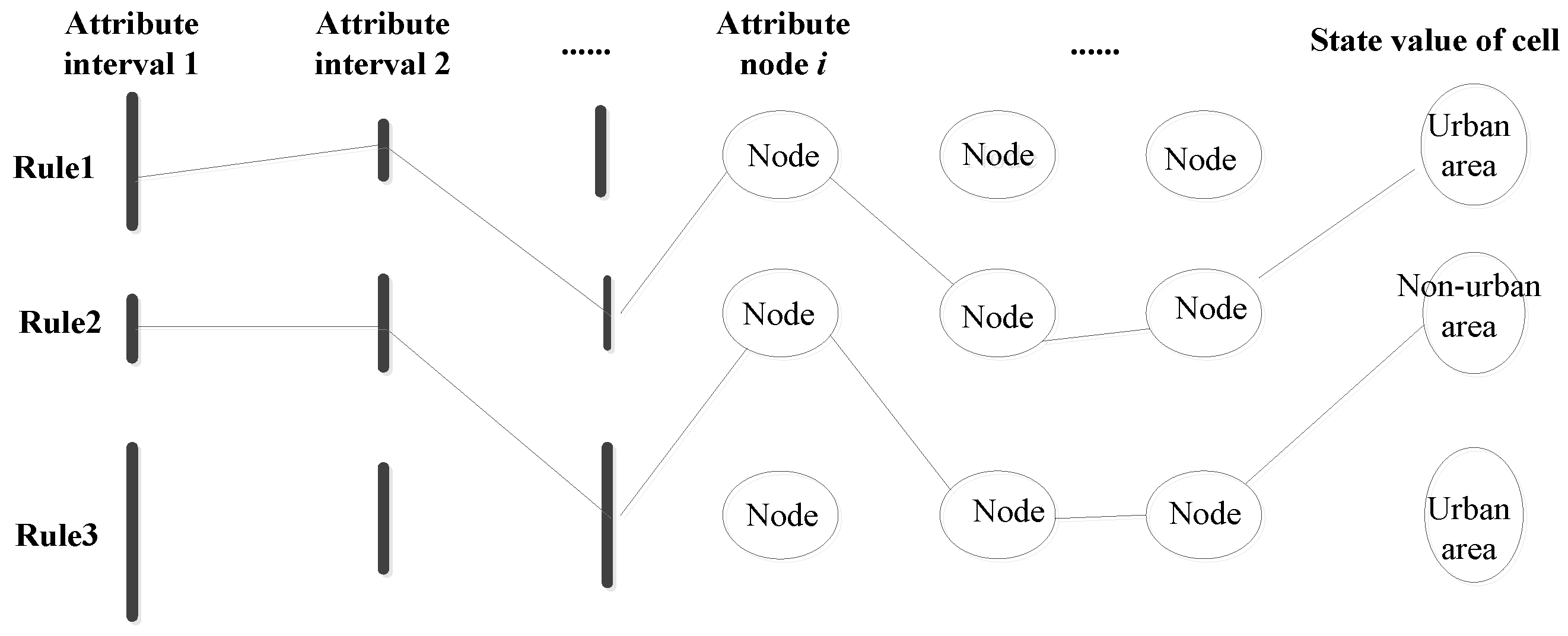
The schematic diagram of the interval model based on CA is shown in Figure 1. The optimized transition rules can be discovered by the CA model, and a transition rule is constructed by a cell state value and attributes’ intervals, each of which is defined by a lower and an upper threshold value for each attribute. The specific construction steps of the CA interval model are described as follows:
(1) Select a value interval (continuous attribute value) or a single attribute node (discrete attribute value) with definite upper and lower bounds on each attribute of the cell.
(2) Logically join and connect a set of selected intervals and nodes, and generate a set of conditions.
(3) Generate a cell state value for a set of conditions combination, and form a complete rule by combining the conditions and the cell state value.
4.2.2. Normalization Processing
Because the ranges and types of attribute values of different geographic features are not the same, if mining the transformation rules using the model on the original attributes’ values of the geographic features, it will result in the wrong rules or the model will not work. Therefore, it is necessary to normalize the values of feature attributes. The specific normalized formula is shown in Equation (5) [35].
where are the original value of feature attribute and the new value after normalization, respectively; and are the minimum value and maximum value of interval of feature attribute, respectively. In addition, the normalization equation normalizes the value interval of the attribute to [0, 1] for easy comparison and calculation. As shown in Figure 2, after the normalization of the values of discrete and continuous attributes by Equation (5), the model can be used to process all attribute values or variables in the same manner.
4.3. Conversion of Interval Model based on CA
After the processing of the CA model, a set of the transition rules for the problem can be mined. To facilitate understanding and processing, the transition rule that is mined by the CA model could be represented by the following reasoning [37].
where n is the number of attributes; the Lower_k and Upper_k are the best lower and the best upper threshold value of the interval on the k-th attribute, respectively, ; Ci refers to a cell status value ; and m is the number of cell state.IFAttribute1 ≥Lower_1 and Attribute1 ≤ Upper_1AndAttribute2 ≥Lower_2 and Attribute2 ≤Upper_2And......AndAttributen ≥Lower_n and Attributen ≤ Upper_nTHENCell state is Ci
Thus, the CA model can be divided into two parts: attribute conditions and cell state. The rule optimization by the optimization algorithm is only conducted on the attribute conditions. To process the model in the computer program, the attribute conditions is expressed as a one-dimensional vector, that is, cell feature vector that is described in Equation (6).
where n is the number of attributes; and are the best lower threshold value and the best upper threshold value of the interval on the kth attribute, respectively. Then, the process of mining conversion rules turns to the process of optimizing the corresponding cell feature vector X for a specific dominant cell state.
5. CA Rule Mining Algorithm based on MHABC Algorithm
In this section, the MHABC algorithm is introduced into the CA model to construct an improved rule mining algorithm MHABC-CA, which can discover optimized transition rules by simulating the behaviors of a swarm of bees. As we mentioned above, a transition rule is constructed by a cell state value and its intervals defined by a lower and an upper threshold value for each attribute. According to the CA transformation model, the process of mining transformation rules is a process of optimizing the corresponding cell feature vector X for a specific advantage cell state. Therefore, the MHABC algorithm can help the CA model find the best lower and upper threshold values of the intervals in each attribute, and mine a set of transition rules. Therefore, the data mining for a transition rule can be regarded as a process of searching for optimal food sources in the MHABC-CA model.
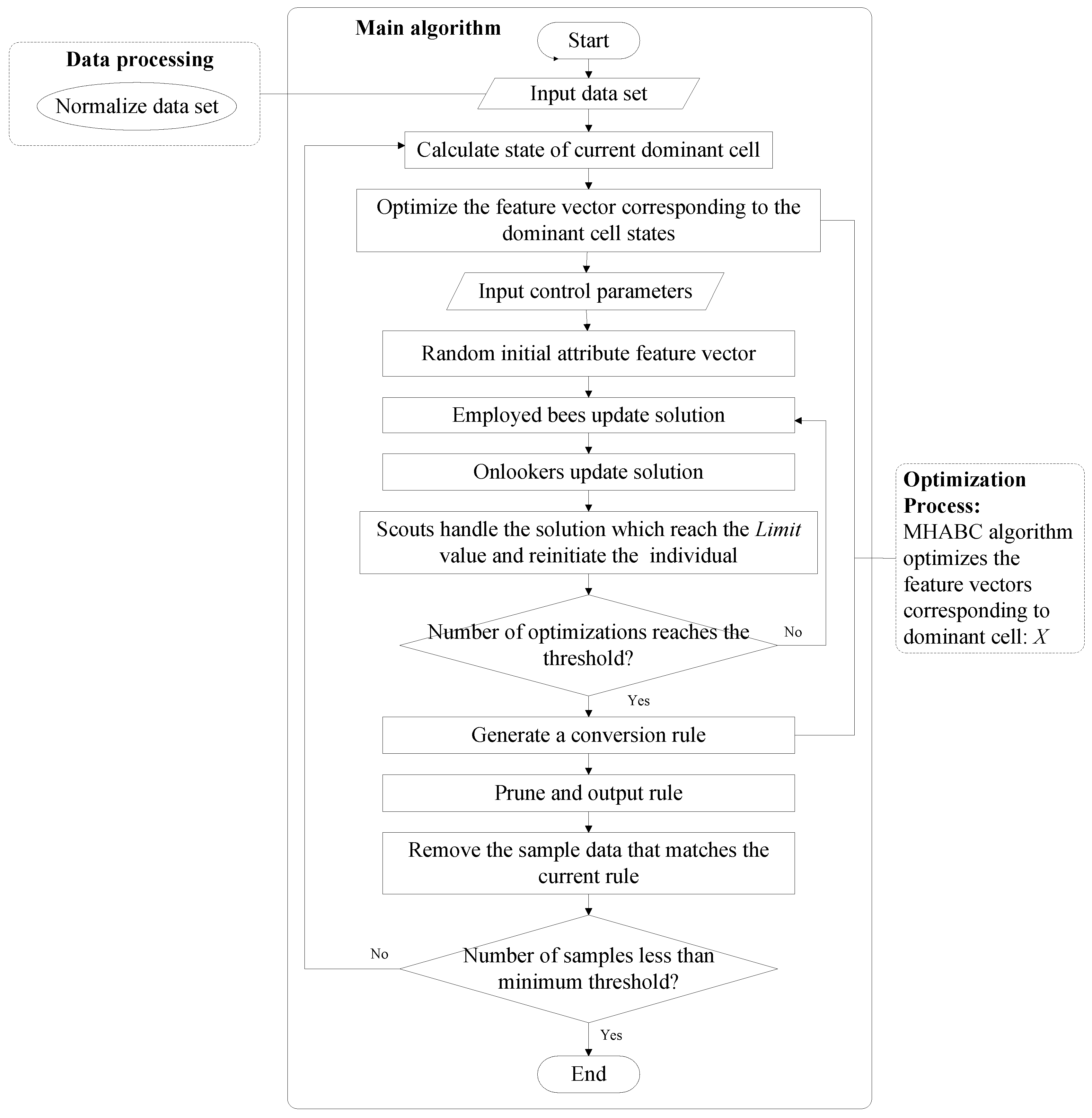
The main steps of MHABC-CA model can be drawn as follows: firstly, it obtains and preprocess the remote sensing images and land-use type data, and converts them into cellular feature vectors by the CA model. The feature vector corresponding to the current dominant cell is calculated. Secondly, the optimization process invokes the improved MHABC algorithm to optimize the feature vector and obtain a conversion rule. Finally, pruning is done on the complete conversion rule to improve its quality. The current dominant cell denotes the optimization solution, which is optimized by the MHABC optimization algorithm, and is chosen according to the fitness function values of the solutions.
The flow chart of MHABC-CA algorithm is shown in Figure 3. The algorithm is mainly divided into three parts. The first part is data processing, which is mainly to preprocess the remote sensing data and to normalize data of different types. The second part is the main algorithm, which is to calculate the states of the dominant cells, and to call the optimization algorithm to operate and perform the rule pruning. The third part is the optimization algorithm, which is to optimize the feature vector X corresponding to a dominant cell based on the MHABC algorithm.
To describe the algorithm more clearly, the pseudocode of MHABC-CA is given in Algorithm 1.
| Algorithm 1. MHABC-CA algorithm. |
| SwarmNumber: Number of bee swarm. FoodNumber: Number of foods sources. FoodNumber = SwarmNumber/2. Trial: Stagnation number of a solution. Limit: Maximum number of trial for the scouts to abandon a food source, and re-initiate a new solution. MFE: Maximum number of iterations. As the number of iterations reaches this value, the iteration process of algorithm will be stopped. MSN: Minimum number of samples. As the number of samples lower than this value, the mining process will be stopped. Begin Input pre-processed data_set; While (Number of samples > MSN) Calculate state of current dominant cell C; For iter = 1 to MFE Input control parameters; Initialization; SendEmployedBees(); SendOnlookerBees(); SendScoutBees(); End For best_rule = GenConvRule(); // Generate a conversion rule. PruneRule(best_rule); // prune the unnecessary conditions from the current rule. UpdateDataSet(data_set, best_rule); // remove the sample data that matches the current rule. UpdateRuleSet(RulesSet, best_rule); // update the current rule into the rules set. End While Return RulesSet; // return and output the rules set. End Function SendEmployedBees() Begin For i = 0 to FoodNumber − 1 Generate a crossover probability cr in the range of [0, 1]; If rand (0, 1) <= cr new_rule = BinaryCrossover(Rule(i)); // crossover operation with the global optimal value Else new_rule = GenNewRule(Rule(i)); // generate a new candidate rule End If If fitness(new_rule) > fitness(Rule(i)) // Calculate and compare the fitness value Rule(i) = new_rule; // Update the rule by the new rule. Trial[i] = 0; // Reset its Trial to 1 Else Trial[i] = Trial[i] + 1; // Increase its Trial by 1 End If End For End Function SendOnlookerBees() Begin index = 0, t = 0; Prob = CalculateProb(); // Calculate the select probabilities of each solution; While (t < FoodNumber) If rand (0, 1) >= Prob(index) new_rule = Mutation (Rule(index)); // mutation operation with the global optimal value Else new_rule = GenNewRule(Rule(index)); // generate a new candidate rule End If If fitness(new_rule) > fitness(Rule(index)) // Calculate and compare the fitness value Rule(index) = new_rule; // Update the rule by the new rule. Trial[index] = 0; // Reset its Trial to 1 Else Trial[i] = Trial[i] + 1; // Increase its Trial by 1 End If End While End Function SendScoutBees() Begin index = 0; For i = 1 to FoodNumber − 1 If Trial(i) > Trial(index) Index = i; End If End For If Trial(index) > Limit Re-Initialize(rule(index)) Trial(index) = 0 End If End |
5.1. Data Processing of MHABC-CA Algorithm
For the CA model in the application of geography, because of the complexity and irregularity of the geographical area, the study area needs to be divided into grids. This paper samples the high-resolution remote sensing images and urban land use type maps of Dengzhou city, and extracts the feature values of attributes and the corresponding cells’ values. However, the inconsistent data types of the sampling data leads to the need for normalization processing of data to ensure the smooth progress of mining.
5.2. Optimization Process of MHABC-CA Algorithm
The optimization process of the MHABC-CA algorithm is to optimize the feature vector X corresponding to a dominant cell state based on the MHABC optimization algorithm. Therefore, in the algorithm processing, optimization is the core step of the algorithm. The special symbols involved in the optimization algorithm are briefly described in Table 1.
In the optimization process of the algorithm, the feature vector X is analogous to the position of nectar source in the ABC algorithm. The optimization process of the feature vector is analogous to the honey-collecting process in the ABC algorithm. Therefore, the optimization process of the feature vector of attributes is as follows.
(1) Bee colony initialization (i.e., feature vector initialization of cell).
The algorithm calls the operation of the optimization algorithm. The SN feature vectors are generated by the random number function, and the dimension is set to 2*n. Simultaneously, the feature vector of each cell is initialized. The specific generation method is described in Equation (7).
where are the lower bound value and the upper bound of the interval on the k-th feature of the i-th cell feature vector, respectively; is a random number function that generates a random number between 0 and 1. When , exchange the values of both. After the feature vectors are initialized, the quality of the cell feature vectors, that is, the quality of the conversion rules generated by the current cell states, is calculated. The initial positions of nectar of the employed bees are the feature vectors that ranked in the top ne.
The Gini index [38] is taken as the quality evaluation method of a transition rule in this paper. Thus, instead of measuring the nectar amount in original ABC algorithm, the fitness function is used for the classification, which is defined in Equation (8).
where TP (true positives) is the number of records covered by the rule that have the class predicted by the rule; FN (false negatives) is the number of records not covered by the rule, but they have the class predicted by the rule; FP (false positives) is the number of records covered by the rule, but their class is not predicted by the rule; TN (True negatives) is the number of records not covered by the rule and that do not have the class predicted by the rule. A higher value of fitness indicates higher quality of the transition rule.
(2) Employed bees stage: Generate the crossover probability cr in the range of [0, 1], and generate a random number rand in the range from 0 to 1. If , the current solution performs the crossover operation with the feature vector X corresponding to the dominant cell state according to Equation (9). Otherwise, the solutions are updated according to the search formula in the basic ABC algorithm.
where are the lower bound value and the upper bound of the interval on the new honey position searched for in the k-th feature near the i-th honey source position (i.e., cell feature vector), respectively; is a random number between [0, 1]; is the global optimal value so far and also is the optimal value of the j-th iteration; and j is the iteration number of the optimization algorithm.
After completing the solutions updating, if , then let ; if , let ; and if , then exchange their values.
(3) Onlookers stage. After completion of the optimization process of employed bees, the following probabilities P of Onlookers are calculated based on the profitability of the employed bees’ positions according to Equation (10).
where fitness is the profitability function of the nectar position of solution X; P(Xi) is the following probability that the i-th employed bee is selected. If the following probability P is greater than the generated random number, the Onlooker searches for a new nectar position near the current nectar position, and the specific search process is similar with the employed bee. Otherwise, the mutation method of inferior solutions is applied for the current nectar position according to Equation (1), and the new mutation position performs its search task according to Equation (9).
After searching for a new position, the qualities of cell feature vectors in this iteration are compared to select the feature vector with the best quality as the optimal solution for this iteration optimization. Then, the optimal solution is compared with the one of the previous iterative optimization, and the one with the higher quality is updated as the new optimal solution. The algorithm continues the optimization process of next iteration.
(4) Scouts stage. According to the basic principle of the ABC algorithm, the abandonment counters of iterations of all employed bees are compared, and the largest number of non-improvement iterations is denoted as abs. Then, the abs is checked with a predefined Limit. If , the related employed bee attached to the nectar position is converted into a Scout bee. The initialization operation is called to generate a new random nectar position and the abandonment counter is reset. The scout bee then becomes employed bee.
(5) Recording the optimal solution.
The algorithm records the optimal solution in the iteration. If the iteration number is greater than the maximum iteration number of the algorithm, the optimization algorithm ends the run.
5.3. Pruning Rule and Updating Sample Set
(1) Pruning of conversion rules
Rule pruning is to remove the unnecessary condition items in the conversion rules to improve its quality. Therefore, a rule pruning method is constructed in this paper, and its specific steps are as follows: removes each condition item in the conversion rule in turn, and calculates the rule’s quality. If the quality is reduced, then returns the removed condition item. On the contrary, removes the condition item. Repeat the rule pruning until removing any of the condition items will reduce the quality of the rule.
(2) Updating of the sample set
To avoid the repeated mining for a dominant sample, a sample updating method in the literature [39] is introduced to remove the sample data from the dataset that matches the current rule. This method can improve the efficiency of the mining process, and improve the quality of the sample set.
6. Case Study of MHABC-CA Algorithm
6.1. Selection of Study Area
6.1.1. Study Area
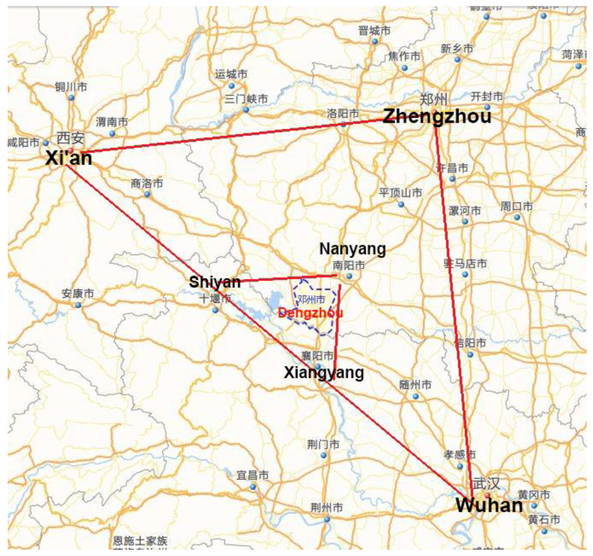
Dengzhou City is a famous historical and cultural city in China. It is the central city of the Danjiangkou Reservoir area, and is also the canal head city of the south-to-north Water Transfer Project designated by the State Council. As shown in Figure 4, from the geographical point of view, Dengzhou is located near the large triangle cities of Wuhan-Xi’an-Zhengzhou and the small triangle cities of Nanyang–Xiangyang–Shiyan. Thus, it plays a “bridge” role in these cities. Dengzhou has a total area of 2369 square kilometers, with 28 townships (streets and districts). The total population is 1,771,200 (2016), and the permanent population is 1,434,700, of which the urban population is more than 400,000 and the urbanization rate is 36.62%. The area marked by the blue short broken lines in the Figure 4 is Dengzhou City.
The geomorphology of Dengzhou city is characterized by few mountains and wide plains. The terrain is flat, the traffic is well developed, and the urban development is mainly influenced by traffic factors. Taking full account of the actual situations, the experimental verification of the MHABC-CA algorithm is mainly carried out to forecast the land use change from 2010 to 2015 in Dengzhou city.
6.1.2. Road Network Data
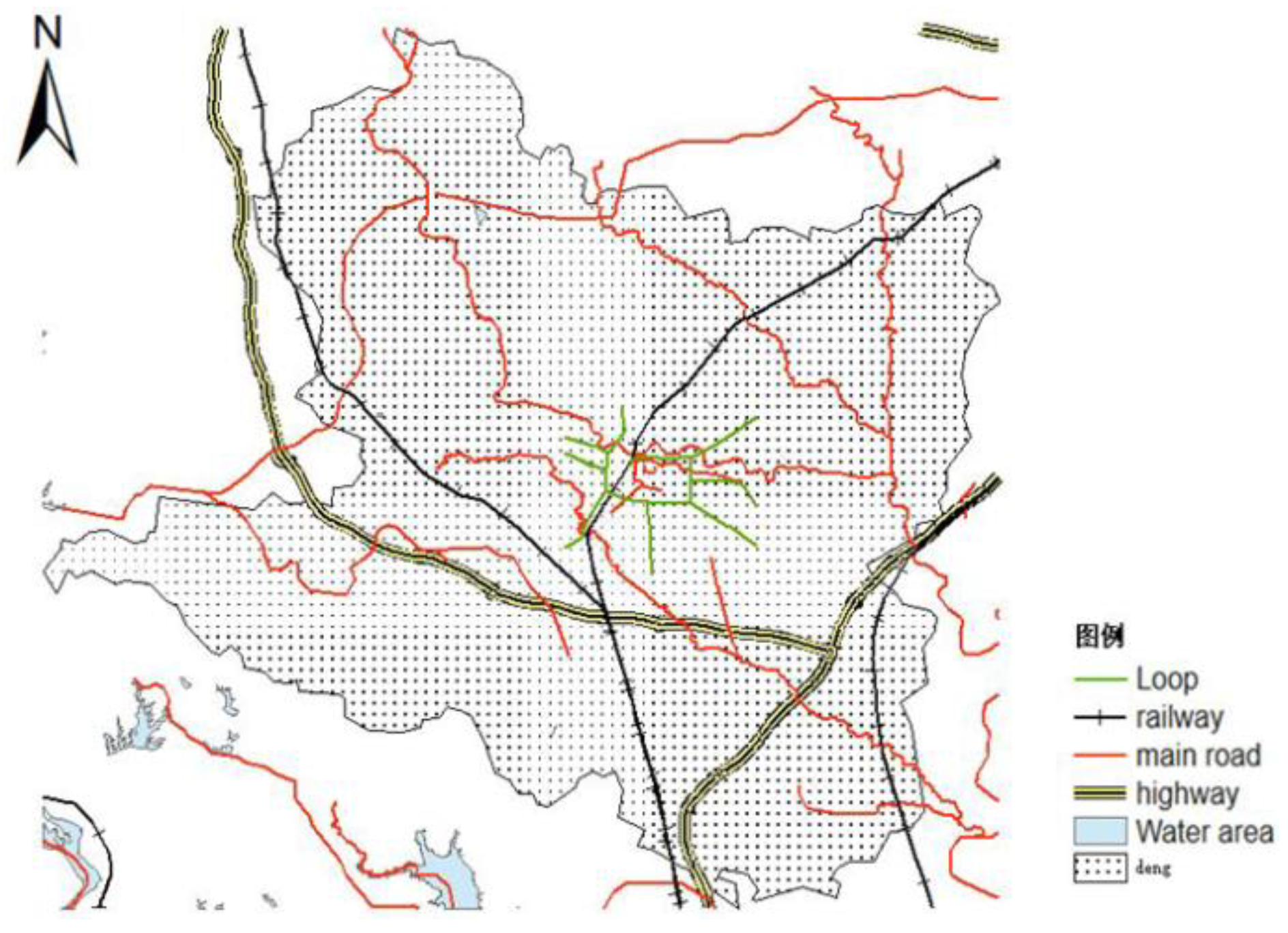
In Dengzhou city, the Jiaoliu Line transits and sets up Dengzhou Station. The highway Erenhot–Guangzhou G55 and the highway from Neixiang to Dengzhou in Henan Province have been built and passed through. The Luoyang–Zhanjiang railway, the Mengxi–Huazhong railway, and the Zhengzhou–Chongqing high-speed railway both transit and set up stations. National Road 207 passes by the Dengzhou, and the National Road G328 and Provincial Highways S231, S335, S249, S248, and S244 all transit through the city. As show in Figure 5, these traffic lines form a three-dimensional traffic network in Dengzhou.
6.1.3. Urban Land Use Type
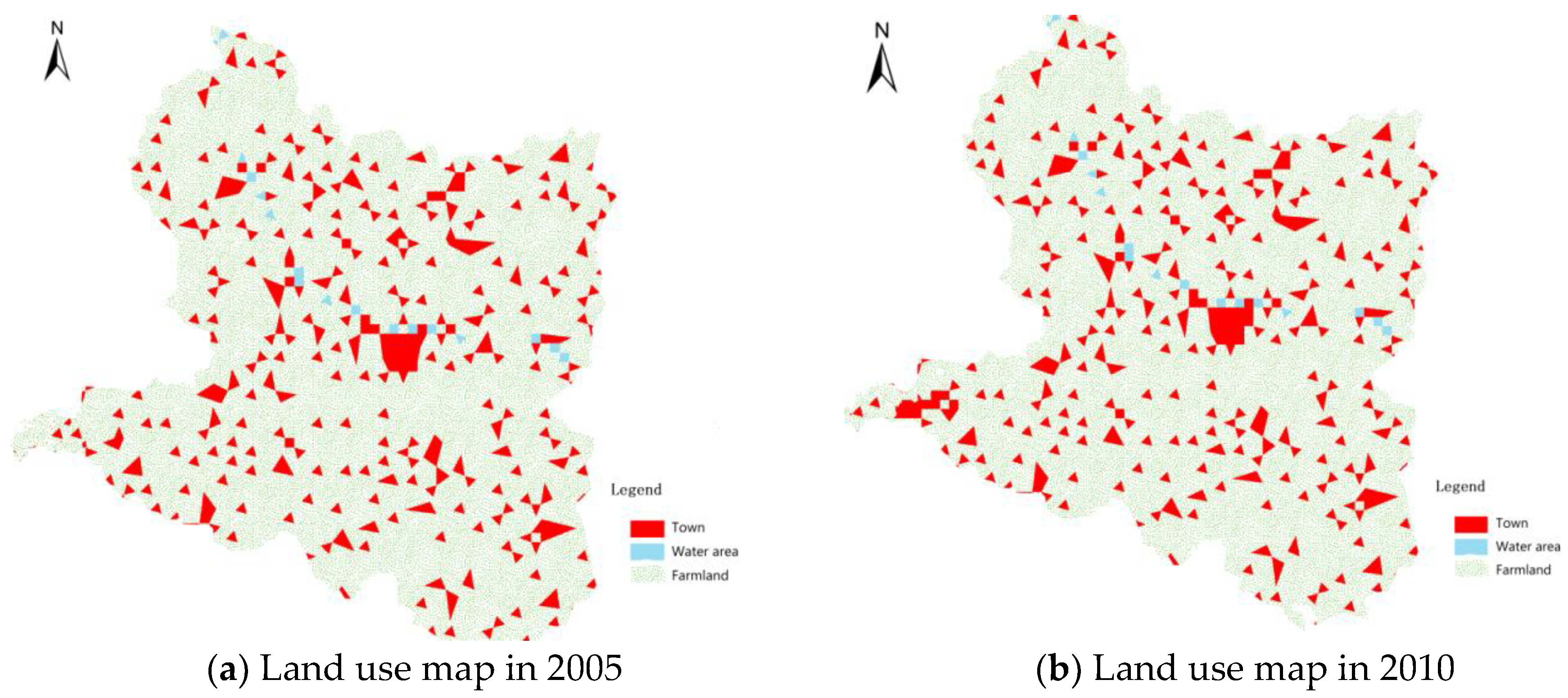
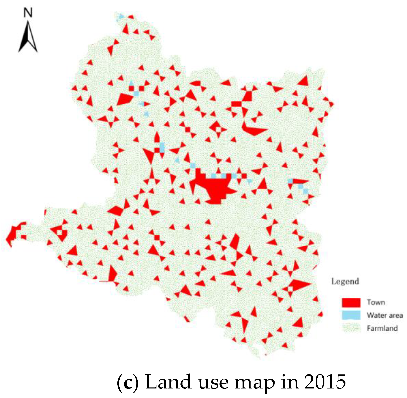
High definition remote sensing images of Dengzhou city in 2005, 2010, and 2015 were obtained. The remote sensing image of Dengzhou city in 2015 is shown in Figure 6. Then, the ArcGIS geography software was used to extract the land use types from these images. The maps of land use types in 2005, 2010, and 2015 were generated, which are shown in Figure 7a–c, respectively. Because Dengzhou city is mainly dominated by agriculture, for simplification of the experiments, we classify its land use into three types: towns (urban), farmland, and water area, with the latter two types being classified as non-urban.
As regular grids are the working basis of the cellular automata model, it is necessary to rasterize the image data by the ArcGIS software in the paper. Taking into account the actual area and building density of Dengzhou city, the image data is rasterized with 50 × 50 m resolution. In the case study, the prediction of urban land use type was studied to verify the effectiveness of the MHABC-CA algorithm and the distance variables of traffic road were taken as the main factors which affecting urban development.
6.2. Data Pre-Processing
Considering the purpose of the experiment and the availability of experimental data, this study selected the traffic distance data of Dengzhou city and used ArcGIS software to extract the required spatial distance variable data. Thus, six spatial distance variables including railways, highways, national roads, provincial roads, urban loops, and the number of cells were selected for this study. The descriptions, ranges, and standardized range of these distance variables are summarized in Table 2. For the CA model, each cell attribute feature is represented by a spatial distance variable.
The spatial analyst module in ArcGIS software was used, and the [Distance][Straight Line] tool in the module was called to calculate the distances from the cell center to the traffic roads, and to obtain the values of the six different spatial distance variables of traffic roads. Before the specific mining experiment, data need to be sampled for regulatory mining. To ensure the rationality of the experimental data, a stratified random sampling method was used in this paper, and 12,044 sample points were extracted from the image of 2005 and 2010 for rule mining experiments.
In this paper, the sampling tool [Sample] in ArcGIS software is used to extract the corresponding sample of these spatial distance variables. Some extracted sample data is shown in Table 3. A complete sample data consists of cell attribute’s features (i.e., the six types of spatial distance variables in Table 2) and cell state value. The value set of cell state is {0, 1}. If a cell transforms into an urban cell, its development status (denoted as DEV _STATUS) will be identified as 1, otherwise it will be identified as 0.
The above sample data was adopted as the experimental data, and then MHABC-CA algorithm was used to mine the rules of urban land use change in Dengzhou city to verify the effectiveness of the MHABC-CA algorithm.
6.3. Prediction Experiment of Urban Land Use Type
The selection of algorithm parameters can greatly affect the execution performance, thus, before taking the MHABC-CA algorithm to mine the rules for prediction of urban land-use type, the algorithm parameters should be identified. The parameters settings of MHABC-CA algorithm, which adopted the recommended parameter from the related researches and our previous experiments results, are shown in Table 4. In the ABC algorithm, the Limit parameter is one of the important parameters, and it is recommended to be performed for tuning or control in literature [40]. However, an extensive parameter tuning is too expensive and also is not the focus of this paper, so we adopted the recommended formula Limit = SN × D [41], where SN is the number of food sources and D is the dimension of a problem, that is, the dimension of the cell feature vector 2 × n. In this paper, we selected six features to mine the rules for urban development. Thus, n is 6, Limit = 20 × 2 × 6 = 240. To facilitate the calculation and evaluation, we set the Limit parameter value to 250 in the experiments.
The MHABC-CA algorithm reads the sample data file, and calculates the state of current dominant cell. Then, according to the parameter setting of the algorithm, the MHABC optimization algorithm will optimize the mining process for conversion rule. As the corresponding conversion rule is generated from the sample data, the pruning method is used to trim the rule, and the sample data that matches the current rule will be removed. In the study, 23 conversion rules are mined using the MHABC-CA algorithm, and partial conversion rules are shown in the following reasoning.
| IF DIST_TL < 6955.7 and DIST_GS > 1674.4 and DIST_GD < 280.0 and DIST_SD < 6771.5 and DIST_HL < 3183.1 and NEIGHBOR < 21.5 THEN DEV STATUS = I IF DIST_TL < 345.55 and DIST_GS > 8700.35 and DIST_GD < 80.25 and DIST_SD < 1771.5 and DIST_HL < 383.1 and NEIGHBOR < 30.2 THEN DEV STATUS = 0 IF DIST_TL < 996.15 and DIST_GS > 364.4 and DIST_GD < 890.0 and DIST_SD < 3771.5 and DIST_HL < 183.1 and NEIGHBOR < 27.3 THEN DEV STATUS = I ...... |
For the above conversion rule, whether the cell meets one of the rules determines whether it will switch its cell state at the next stage. The form of conversion rules in upper reasoning is not easily understood. Thus, we take the first rule as an example to describe its meanings as follows; if the distance from the cell to the railway is less than 6955.7 m, the distance from the cell to the highway is less than 1674.4 m, the distance from the cell to the national road is less than 280 m, the distance from the cell to the provincial road is less than 6771.5 m, the distance from the cell to the urban loop is less than 3183.1 m, and the number of urban cells in the 7 × 7 neighborhood window is less than 21.5, then the state value of the cell is 1, which indicates that the cell will be converted to a urban state at the next stage. On the contrary, for the second rule, if the distance from the cell to the railway is less than 344.55 m, the distance from the cell to the highway is less than 8705.35 m, the distance from the cell to the national road is less than 80.25 m, the distance from the cell to the provincial road is less than 1771.5 m, the distance from the cell to urban loop is less than is less than 383.1 m, and the number of urban cells in the 7 × 7 neighborhood window is less than 30.2, then the state value of the cell is 0, which indicates that the cell will be converted to non-urban areas in the next time. With continuous iteration simulation, the urban land use conditions of Dengzhou city in 2015 can be simulated by the MHABC-CA algorithm.
6.4. Analysis of Simulation Results
The mining quality of the MHABC-CA algorithm can be tested by conducting comparative tests and analysis for the simulated results and actual situation of urban land use of Dengzhou city in 2015. Therefore, two analysis methods, visual characteristics of urban land use types and quantitative simulation accuracy, were done in the paper.
6.4.1. Comparison of Visual Features
Visual features are people’s intuitive visual perception to images. Therefore, comparing the visual features of simulated results images with actual images is the most intuitive and simple analytical method for testing simulation results [42]. The comparison of visual features allows us to conduct a more comprehensive verification and analysis of the simulation results of the MHABC-CA algorithm. Although there is a certain degree of subjectivity, the analysis method has certain significance on the experimental results.
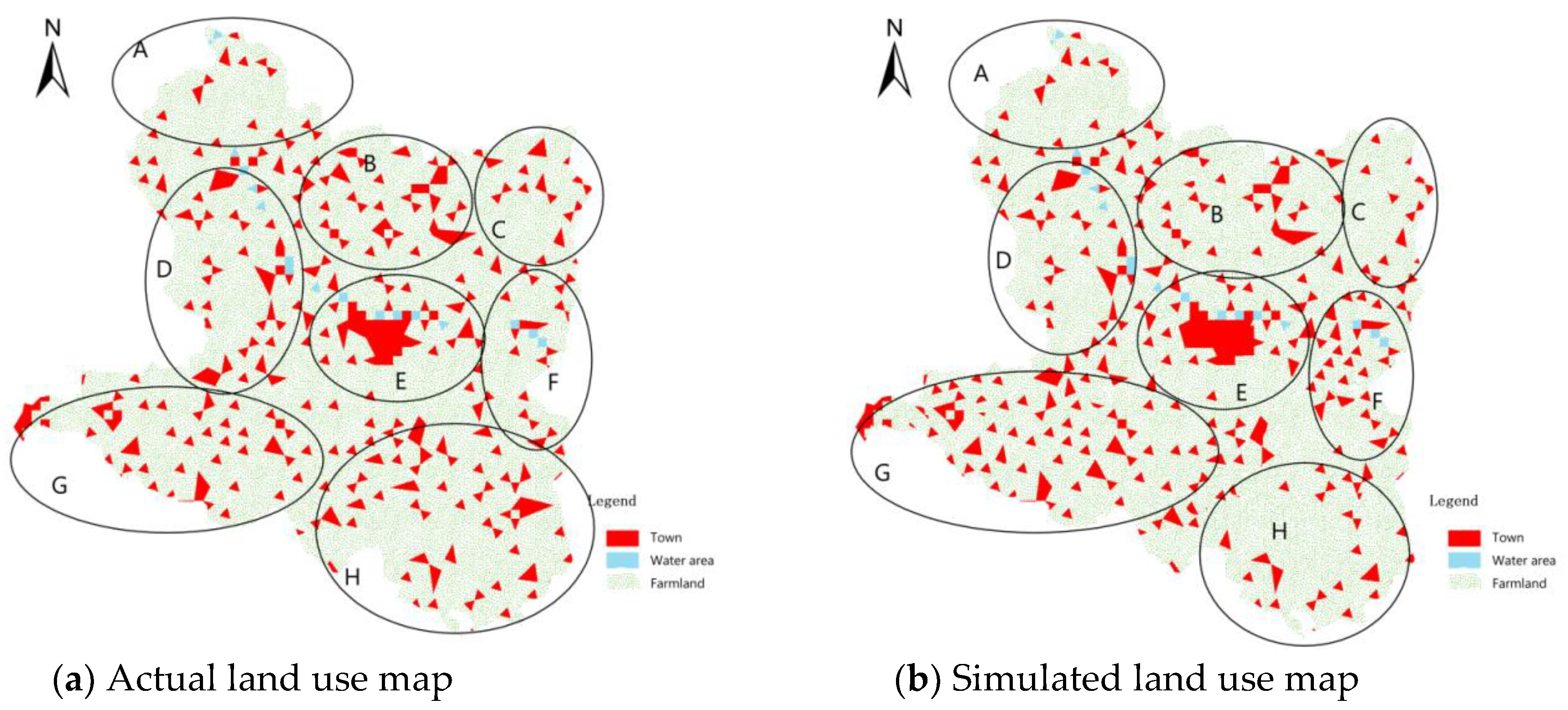
As shown in Figure 8, the (a) and (b) are the actual and the simulated land use maps of Dengzhou city for 2015, respectively. The urban area of Dengzhou city is divided into eight regions, A, B, C, D, E, F, G, and H, in this paper. The detailed descriptions are as follows:
Area A is the northeast corner of the city. The simulation results of MHABC-CA algorithm are very close to the actual situation. There is no case of over-fitting and insufficient simulation.
Area B is the true north side of the city. The simulation results of MHABC-CA algorithm are basically same as the actual situation, but the simulation is insufficient.
Area C is the northwest corner of the city. The simulation results of MHABC-CA algorithm are basically same as the actual situation, but there is serious insufficient simulation.
Area D is the west side of the city. The simulation results of MHABC-CA algorithm are consistent with the actual situation.
Area E is the core urban area of the city. The simulation results of MHABC-CA algorithm are basically same as the actual situation, but the simulation results are over-fitted.
Area F is the east side of the city. The simulation results of MHABC-CA algorithm are basically inconsistent with the actual situation, and there is a certain problem of over-fitting.
Area G is the southwest corner of the city. The simulation results of MHABC-CA algorithm are basically same as the actual situation, but there is a certain degree of over-fitting.
Area H is the southwest corner of the city. The simulation results of MHABC-CA algorithm are basically same as the actual situation, but there is a certain degree of insufficient simulation.
In summary, although there is a certain degree of over-fitting simulation and insufficient simulation, the simulated urban land use situation predicted by the MHABC-CA algorithm is basically consistent with the actual situation of Dengzhou city, and the simulation can achieve the predicted effect from the view of visual features method.
6.4.2. Quantitative Analysis of Simulation Accuracy
The subjective influence of the comparison method of visual features is relatively large, so we want to adopt a quantitative analysis method to analyze and compare the changes of urban land use types. The error matrix is a standard method that can represent the data accuracy, which is represented by a matrix of n rows and n columns [43]. The error matrix can be applied to the MHABC-CA model to analyze its simulation accuracy. In the matrix, the number of cells of urban land use in the actual situation and the simulated results are both recorded as a; the number of cells in the simulation result is urban land, but not urban land in the actual situation, is recorded as b; the number of cells that neither in the simulation results nor in the actual situation are urban land is denoted as c; and the number of cells that are not the urban land in the simulation results, but are the urban land in the actual situation, is denoted as d. Then, the error matrix can be used to calculate the quantitative simulation accuracy of the MHABC-CA algorithm, and the specific calculation method is shown in the Table 5.
To compare the simulation accuracy of the MHABC-CA algorithm with other algorithm, we introduced a cellular automata model based on particle swarm optimization (PSO-CA) algorithm. Similar to MHABC-CA rule mining algorithm, the method of mining a rule based on PSO-CA rule mining algorithm is also to find the optimal cell feature vector for a specific cell state. The cell feature vector is the position of the particle of PSO algorithm in the search space. Similar algorithms can also be found in the literature, for example, Feng et al. presented an improved cellular automata (CA) model of urban growth based on particle swarm optimization (PSO) approach with inertia weight, and the model was applied in Fengxian District of Shanghai Municipality, eastern China, to simulate the spatial-temporal process of urban growth from 1992 to 2008 at 30 m spatial resolution [44]; and Rabbani et al. presented a hybrid cellular automata (HCA) model with PSO algorithm, and applied it to landsat satellite imagery of the city of Tehran, Iran with 28.5-m spatial resolution to simulate the urban growth from 1988 to 2010 [45].
In the comparison experiments, an assumption that fitness evaluation is time-consuming and much bigger than algorithm internal calculations has been made, thus, the usual manner is to compare them on equal number of fitness evaluations consumed [46,47]. For the PSO algorithm, the population size (SN2) is 50, and c1 = c2 = 1.108, and w = 0.721 [48]. The maximum number of iterations (MFE1) of MHABC-CA is 2500, and the maximum number of iterations (MFE2) of PSO-CA is 2050. Therefore, the maximum number of fitness evaluations of MHABC-CA algorithm is (SN + SN + 1) × MFE1 + SN = 102,520, and the maximum number of fitness evaluations of PSO-CA algorithm is SN2 × MFE2 + SN2 = 102,550. The two algorithms have a similar number of fitness evaluations. Then, each of the algorithms was repeated 30 times independently to analyze the experiment results.
To compare the execution performance of MHABC-CA algorithm and PSO-CA algorithm, the execution time (unit: Second) was statistically calculated in Table 6 and Table 7. Max, Min, Mean, and SD represent the maximum value, minimum value, average value, and the standard deviation of the experiments results, respectively. The results showed the MHABC-CA algorithm can have the similar performance in execution time under the same operating conditions.
For the validation phase, the validation results should exclude the areas that are resistant or excluded to development at the initial time, because those areas are not candidates for simulated change [49,50]. The excluded areas from development consisted of water, wetlands, government, and local parks, among others [51]. Then, evaluation was performed by excluding the excluded areas in which land uses remain constant. The experimental data of MHABC-CA algorithm were put into the error matrix in Table 5, the simulation accuracy results for the urban land use prediction of Dengzhou city in 2015 was calculated, and the optimal results are shown in Table 7 and Table 8. The optimal simulation accuracy results of PSO-CA algorithm in error matrix form is shown in Table 8. The comparison of experiments results validates the effectiveness of the MHABC-CA algorithm, and demonstrates that it achieves better simulation accuracy than the PSO-CA algorithm.
7. Conclusions
Conventional raster-based cellular automata models confront many problems, and studies demonstrated that the swarm intelligence algorithms are suitable to search for the global optimum parameters of transition rules for CA models. Thus, an improved artificial bee colony algorithm named MHABC is introduced into the cellular automata interval model to construct a new effective CA rule mining algorithm (MHABC-CA) for modeling urban dynamics in this paper. Then, the urban land use prediction of Dengzhou city of Henan Province is taken as the case study to verify the effectiveness of the algorithm.
We obtained three phases’ remote sensing data of Dengzhou city in 2005, 2010, and 2015, and six spatial distance variables including railways, highways, national roads, provincial roads, urban loops, and the number of cells were extracted from these data and were taken as the major factors. The simulation results, evaluated with visual characteristics of urban land use types and quantitative simulation accuracies, demonstrate that the MHABC-CA model outperforms other spatial statistical based CA models. The new CA parameters retrieved by the MHABC algorithm can stochastically optimize the transition rules to reduce the simulation uncertainties and can express precisely the contributions of various driving forces to predict the urban dynamics. In the future work, we will consider the influencing factors of geographical environment and socio-economy, and introduce more factors that affect land use changes to improve mining quality. We also plan to perform a deeply analysis on the node features of CA model, a similar method for complex network analysis can be found in the literature [52].
Author Contributions
Conceptualization, J.H. and Z.Z.; Methodology, J.H.; Software, Z.Z.; Validation, J.H. and Z.Z.; Writing—Original Draft Preparation, Z.Z.; Writing—Review & Editing, J.H.
Funding
This research was funded by National Nature Science Foundation of China (Grant No. 61462058, 61741201).
Acknowledgments
Our deepest gratitude goes to the anonymous reviewers and editors for their careful work and thoughtful suggestions that have helped improve this paper substantially.
Conflicts of Interest
The authors declare no conflict of interest.
References
- Van Vliet, J.; Bregt, A.K.; Brown, D.G.; van Delden, H.; Heckbert, S.; Verburg, P.H. A review of current calibration and validation practices in land-change modeling. Environ. Model. Softw. 2016, 82, 174–182. [Google Scholar] [CrossRef]
- Brown, D.G.; Verburg, P.H.; Pontius, R.G., Jr.; Lange, M.D. Opportunities to improve impact, integration, and evaluation of land change models. Curr. Opin. Environ. Sustain. 2013, 5, 452–457. [Google Scholar] [CrossRef]
- Wang, J.; Lin, Y.; Glendinning, A.; Xu, Y. Land-use changes and land policies evolution in China’s urbanization processes. Land Use Policy 2018, 75, 375–387. [Google Scholar] [CrossRef]
- Dong, N.; You, L.; Cai, W.J.; Li, G.; Lin, H. Land use projections in China under global socioeconomic and emission scenarios: Utilizing a scenario-based land-use change assessment framework. Glob. Environ. Chang. 2018, 50, 164–177. [Google Scholar] [CrossRef]
- Ustaoglu, E.; Castillo, C.P.; Jacobs-Crisioni, C.; Lavalle, C. Economic evaluation of agricultural land to assess land use changes. Land Use Policy 2016, 56, 125–146. [Google Scholar] [CrossRef]
- Blecic, I.; Cecchini, A.; Trunfio, G.A. How much past to see the future: A computational study in calibrating urban cellular automata. Int. J. Geogr. Inf. Syst. 2015, 29, 349–374. [Google Scholar] [CrossRef]
- Yang, H.B.; Du, L.J.; Guo, H.L.; Zhang, J. Tai’an Land Use Analysis and Prediction Based on RS and Markov Model. Procedia Environ. Sci. 2011, 10, 2625–2630. [Google Scholar]
- Fu, X.; Wang, X.H.; Yang, Y.J. Deriving suitability factors for CA-Markov land use simulation model based on local historical data. J. Environ. Manag. 2018, 206, 10–19. [Google Scholar] [CrossRef] [PubMed]
- Veldkamp, A.; Fresco, L.O. CLUE: A conceptual model to study the Conversion of Land Use and its Effects. Ecol. Model. 1996, 85, 253–270. [Google Scholar] [CrossRef]
- Kennedy, J. Swarm intelligence. In Handbook of Nature-Inspired and Innovative Computing; Springer: Boston, MA, USA, 2006; pp. 187–219. [Google Scholar]
- Karaboga, D.; Basturk, B. A Powerful and Efficient Algorithm for Numerical Function Optimization: Artificial Bee Colony (ABC) Algorithm. J. Glob. Optim. 2007, 39, 459–471. [Google Scholar] [CrossRef]
- Kabalci, Y.; Kockanat, S.; Kabalci, E. A modified ABC algorithm approach for power system harmonic estimation problems. Electr. Power Syst. Res. 2018, 154, 160–173. [Google Scholar] [CrossRef]
- Amarjeet; Chhabra, J.K. FP-ABC: Fuzzy-Pareto dominance driven artificial bee colony algorithm for many-objective software module clustering. Comput. Lang. Syst. Struct. 2018, 51, 1–21. [Google Scholar]
- Zhong, F.; Li, H.; Zhong, S. A modified ABC algorithm based on improved-global-best-guided approach and adaptive-limit strategy for global optimization. Appl. Soft Comput. 2016, 46, 469–486. [Google Scholar] [CrossRef]
- Qin, Q.D.; Cheng, S.; Li, L.; Shi, Y.H. A survey of artificial bee colony algorithm. J. Intell. Syst. 2014, 9, 127–135. [Google Scholar]
- Boztoprak, H.; Özbay, Y.; Güçlü, D.; Küçükhemek, M. Prediction of sludge volume index bulking using image analysis and neural network at a full-scale activated sludge plant. Desalination Water Treat. 2015, 57, 1–11. [Google Scholar] [CrossRef]
- Santhi, V.; Nandhini, S. An Efficient Algorithm for Job Scheduling Problem-Enhanced Artificial Bee Colony Algorithm. Asian J. Inf. Technol. 2016, 15, 2210–2216. [Google Scholar]
- Zhu, G.; Kwong, S. Gbest-guided artificial bee colony algorithm for numerical function optimization. Appl. Math. Comput. 2010, 217, 3166–3173. [Google Scholar] [CrossRef]
- Huo, J.Y.; Zhang, Y.N.; Zhao, H.X. An improved artificial bee colony algorithm for numerical functions. Int. J. Reason.-Based Intell. Syst. 2015, 7, 200–208. [Google Scholar] [CrossRef]
- Niu, F.Q.; Li, J. Modeling the population and industry distribution impacts of urban land use policies in Beijing. Land Use Policy 2018, 70, 347–359. [Google Scholar] [CrossRef]
- Amici, V.; Marcantonio, M.; Porta, N.L.; Rocchini, D. A multi-temporal approach in MaxEnt modelling: A new frontier for land use/land cover change detection. Ecol. Inform. 2017, 40, 40–49. [Google Scholar] [CrossRef]
- Zhao, L.Y.; Peng, Z.R. LandSys II: Agent-Based Land Use-Forecast Model with Artificial Neural Networks and Multiagent Model. J. Urban Plan. Dev. 2014, 141, 04014045. [Google Scholar] [CrossRef]
- Huang, T.; Zhang, C.Z. Simulation and Prediction of Land Use Based on the Markov Model. In Proceedings of the 9th International Symposium on Linear Drives for Industry Applications; Springer: Berlin/Heidelberg, Germany, 2014; Volume 2, pp. 373–377. [Google Scholar]
- Anputhas, M.; Janmaat, J.J.A.; Nichol, C.F.; Wei, X.H. Modelling spatial association in pattern based land use simulation models. J. Environ. Manag. 2016, 181, 465–476. [Google Scholar] [CrossRef] [PubMed]
- Li, Z.M.; Song, G.; Lu, S.; Wang, H.; Xu, S.G. Prediction of land use change in Harbin based on CA-Markov model. Chin. Agric. Resour. Reg. Plan. 2017, 38, 41–48. [Google Scholar]
- Huang, P.; Yuan, Y.B.; Dong, H. Study on land use change in Qingjiang basin using CA-Markov model. Surv. Sci. 2017, 42, 102–109. [Google Scholar]
- Zhang, X.J.; Zhou, Q.G.; Wang, Z.L.; Wang, F.H. Land use evolution simulation and prediction based on MCE-CA-Markov in the Three Gorges reservoir area. Chin. J. Agric. Eng. 2017, 33, 268–277. [Google Scholar]
- Yuntana, D.; Su, G.C.; Sun, W.R.; Tu, Y. Land use change analysis based on GIS and CA-Markov model in the Cullen County. J. Yangtze Univ. China 2017, 14, 79–82+85. [Google Scholar]
- Lu, N.; Li, Z.H.; Bao, Y.J.; Li, Z.L.; Zhang, J.; Liu, L.; Liu, X.; Tan, Y.C.; Gong, X.S. Analysis and Prediction of Land Use Dynamic Change Based on CA-Markov Model in Balikun Lake Basin. Tianjin Agric. Sci. 2017, 23, 63–65. [Google Scholar]
- Wang, C.X.; Zhang, C. Land Use Change Prediction Model Based on Genetic BP Neural Network Model. Surv. Mapp. 2017, 40, 52–55. [Google Scholar]
- Zhang, J.P.; Li, J. Prediction and Analysis of Land Use Change in Ganzhou District Based on CA-Markov Model. Chin. Agric. Sci. Bull. 2017, 33, 105–110. [Google Scholar]
- Yu, D.G.; Wu, Q. Research and Application of Multi-factor Driven Prediction Model for Land Use Structural Change based on Logistic-Markov Method. Bull. Soil Water Conserv. 2017, 37, 149–154. [Google Scholar]
- Jiang, M.Y.; Yuan, D.F. Artificial Bee Colony Algorithm and Its Application; Science Press: Beijing, China, 2014. [Google Scholar]
- Huo, J.Y.; Zhang, Z.; Meng, F.M. A hybrid artificial bee colony algorithm guided by mutation strategy. Comput. Appl. Softw. 2018, 35, 267–272. [Google Scholar]
- Yang, J.Y. Research on Mining Methods of Geographic Cellular Automata Transformation Rules Based on Bee Colony Intelligence; Nanjing Normal University: Nanjing, China, 2014. [Google Scholar]
- Li, X.; Ye, J.A.; Liu, X.P.; Yang, J.S. Geographic Simulation System: Cellular Automata and Multi-Agent; Science Press: Beijing, China, 2007. [Google Scholar]
- Yang, J.; Tang, G.; Cao, M.; Zhu, R. An intelligent method to discover transition rules for cellular automata using bee colony optimization. Int. J. Geogr. Inf. Sci. 2013, 27, 1849–1864. [Google Scholar] [CrossRef]
- Shukran, M.A.M.; Chung, Y.Y.; Yeh, W.C.; Wahid, N.; Zaidi, A.M.A. Artificial Bee Colony based Data Mining Algorithms for Classification Tasks. Mod. Appl. Sci. 2011, 5, 217–231. [Google Scholar] [CrossRef]
- Tang, J.; Chai, T.Y.; Liu, Z.; Yu, W.; Zhou, X.J. Adaptive Ensemble Modelling Approach Based on Updating Sample Intelligent Identification. Acta Autom. Sin. 2016, 42, 1040–1052. [Google Scholar]
- Veček, N.; Liu, S.H.; Črepinšek, M.; Mernik, M. On the Importance of the Artificial Bee Colony Control Parameter ‘Limit’. Inf. Technol. Control 2017, 46, 566–604. [Google Scholar] [CrossRef]
- Karaboga, D.; Akay, B.; Ozturk, C. Artificial Bee Colony (ABC) Optimization Algorithm for Training Feed-Forward Neural Networks. Model. Decis. Artif. Intell. 2007, 4617, 318–329. [Google Scholar]
- Yang, X. Research on Visual Feature Expression and Learning for Image Classification and Recognition; South China University of Technology: Guangzhou, China, 2014. [Google Scholar]
- Wang, D.; Li, C.S.; Wu, H. Optimal closed-form solution of array error matrix based on eigenvectors. J. Appl. Sci. 2009, 27, 592–600. [Google Scholar]
- Feng, Y.; Liu, Y.; Tong, X.; Liu, M.L.; Deng, S.S. Modeling dynamic urban growth using cellular automata and particle swarm optimization rules. Landsc. Urban Plan. 2011, 102, 188–196. [Google Scholar] [CrossRef]
- Rabbani, A.; Aghababaee, H.; Rajabi, M.A. Modeling dynamic urban growth using hybrid cellular automata and particle swarm optimization. J. Appl. Remote Sens. 2012, 6, 063582. [Google Scholar] [CrossRef]
- Mernik, M.; Liu, S.H.; Karaboga, D.; Črepinšek, M. On clarifying misconceptions when comparing variants of the Artificial Bee Colony Algorithm by offering a new implementation. Inf. Sci. 2015, 291, 115–127. [Google Scholar] [CrossRef]
- Črepinšek, M.; Liu, S.H.; Mernik, M. Replication and comparison of computational experiments in applied evolutionary computing: Common pitfalls and guidelines to avoid them. Appl. Soft Comput. J. 2014, 19, 161–170. [Google Scholar] [CrossRef]
- Nozohour-Leilabady, B.; Fazelabdolabadi, B. On the application of artificial bee colony (ABC) algorithm for optimization of well placements in fractured reservoirs; efficiency comparison with the particle swarm optimization (PSO) methodology. Petroleum 2016, 2, 79–89. [Google Scholar] [CrossRef]
- Pontius, R.G.; Boersma, W.; Castella, J.C.; Clarke, K.; de Nijs, T.; Dietzel, C.; Duan, Z.; Fotsing, E.; Goldstein, N.; Kok, K.; et al. Comparing the input, output, and validation maps for several models of land change. Ann. Reg. Sci. 2008, 42, 11–37. [Google Scholar] [CrossRef]
- Chen, H.; Pontius, R.G., Jr. Sensitivity of a Land Change Model to Pixel Resolution and Precision of the Independent Variable. Environ. Model. Assess. 2011, 16, 37–52. [Google Scholar] [CrossRef]
- Jantz, C.A.; Goetz, S.J.; Shelley, M.K. Using the SLEUTH Urban Growth Model to Simulate the Impacts of Future Policy Scenarios on Urban Land Use in the Baltimore-Washington Metropolitan Area. Environ. Plan. B Plan. Des. 2004, 31, 251–271. [Google Scholar] [CrossRef]
- Jesenko, D.; Mernik, M.; Žalik, B.; Mongus, D. Two-level Evolutionary Algorithm for Discovering Relations Between Nodes’ Features in a Complex Network. Appl. Soft Comput. 2017, 56, 82–93. [Google Scholar] [CrossRef]
Figure 1.
Schematic diagram of interval model based on cellular automata (CA) [35].
Figure 1.
Schematic diagram of interval model based on cellular automata (CA) [35].

Figure 2.
Schematic representation of the rule after regularization [35].
Figure 2.
Schematic representation of the rule after regularization [35].

Figure 3.
Flow chart of the improved hybrid artificial bee colony algorithm based on the mutation of inferior solutions (MHABC)-CA algorithm.
Figure 3.
Flow chart of the improved hybrid artificial bee colony algorithm based on the mutation of inferior solutions (MHABC)-CA algorithm.

Figure 4.
Geographic location map of Dengzhou city.

Figure 5.
Dengzhou Road Network.

Figure 6.
Remote sensing image of Dengzhou city in 2015.

Figure 7.
Land use maps of Dengzhou city in 2005, 2010, and 2015.


Figure 8.
The actual and simulated land use maps of Dengzhou city for 2015.


Table 1.
The specific meaning of mathematical symbols in the optimization algorithm.
| Symbol | Description |
|---|---|
| SN | The number of food sources (SN = SNe = SNo) |
| SNe | The number of Employed bees |
| SNo | The number of onlookers |
| n | Feature dimension of Cell |
| X | Bee populations of Employed bees, |
Table 2.
The value range of the six spatial distance variables.
| Spatial Variables | Description | Ranges (Unit) | Standardized Range |
|---|---|---|---|
| DIST_TL | The distance from a grid unit to the railway | 0–35,200 (m) | 0–1 |
| DIST_GS | The distance from a grid unit to the highway | 0–56,100 (m) | 0–1 |
| DIST_GD | The distance from a grid unit to the national road | 0–42,100 (m) | 0–1 |
| DIST_SD | The distance from a grid unit to the provincial road | 0–14,400 (m) | 0–1 |
| DIST_HL | The distance from a grid unit to the city loop | 0–35,400 (m) | 0–1 |
| NEIGHBOR | The number of city cells in the 7 × 7 window | 0–49 | 0–1 |
Table 3.
Sample Data.
| DIST_TL | DIST_GS | DIST_GD | DIST_SD | DIST_HL | NEIGHBOR | DEV_STATUS |
|---|---|---|---|---|---|---|
| 362.49 | 108.16 | 7682.46 | 416.77 | 8607.12 | 49 | 0 |
| 8.16 | 41.6.77 | 7682.46 | 48.26 | 3540 | 0 | 0 |
| 48.26 | 5122.53 | 8607.12 | 212.13 | 94.86 | 2 | 1 |
| 108.15 | 4249.52 | 305.941 | 3768.2 | 94.86 | 0 | 1 |
| 5050.34 | 2421.65 | 3703.02 | 7567.19 | 4012.04 | 1 | 0 |
| 4193.35 | 8554.68 | 8554.68 | 228.473 | 342.05 | 1 | 0 |
| 3396.49 | 5023.27 | 23.69 | 4484.47 | 8160.49 | 49 | 1 |
| 254.55 | 27.27 | 254.55 | 816.08 | 300 | 3 | 1 |
| 14,460.78 | 27.27 | 329.45 | 3789.55 | 355.78 | 49 | 0 |
Table 4.
Parameter settings of improved hybrid artificial bee colony algorithm based on the mutation of inferior solutions (MHABC)-cellular automata (CA) algorithm.
Table 4.
Parameter settings of improved hybrid artificial bee colony algorithm based on the mutation of inferior solutions (MHABC)-cellular automata (CA) algorithm.
| Parameter | Value | Description |
|---|---|---|
| Food sources number (SN) | 20 | The number of food sources which is equal to the number of employed or onlooker bees. |
| Individual search limit (Limit) | 250 | If the fitness value of a honey source has not been improved in the number of Limit iterations, the honey source will be discarded. |
| Number of iterations | 2500 | The maximum number of iteration of the algorithm |
| Rule convergence threshold | 500 | The maximum number of convergence rules. |
| Minimum fitting ratio | 0.01 | When the ratio of remaining samples to total number of samples reaches this parameter, the mining algorithm will be stopped. |
| Effective coverage | 0.005 | The ratio of minimum samples to total number of samples that matches a rule which is to control the quality of the rule. |
Table 5.
Simulation accuracy calculation method in the error matrix.
| Urban Land in Actual Situation | Non-Urban Land in Actual Situation | |
|---|---|---|
| Urban land in simulation results | a | b |
| Non-urban land in simulation results | d | c |
| Simulation accuracy | (a + c)/(a + b + c + d) × 100% | |
Table 6.
Execution performance comparison of MHABC-CA algorithm and particle swarm optimization (PSO)-CA algorithm.
Table 6.
Execution performance comparison of MHABC-CA algorithm and particle swarm optimization (PSO)-CA algorithm.
| Algorithm | Execution Time (Unit: Second) | |||
|---|---|---|---|---|
| Max | Min | Mean | SD | |
| PSO-CA | 1.013 × 10² | 9.677 × 101 | 9.886 × 101 | 4.021 × 100 |
| MHABC-CA | 1.098 × 10² | 9.733 × 101 | 1.034 × 10² | 3.475 × 100 |
Table 7.
Simulation accuracy results of MHABC-CA algorithm in error matrix form.
| Urban Land in Actual Situation | Non-Urban Land in Actual Situation | |
|---|---|---|
| Urban land in simulation results | 34,168 | 5796 |
| Non-urban land in simulation results | 7557 | 42,029 |
| Simulation accuracy | 85.09% | |
Table 8.
Simulation accuracy results of PSO-CA algorithm in error matrix form.
| Urban Land in Actual Situation | Non-Urban Land in Actual Situation | |
|---|---|---|
| Urban land in simulation results | 32,285 | 7833 |
| Non-urban land in simulation results | 8684 | 40,748 |
| Simulation accuracy | 81.56% | |
© 2018 by the authors. Licensee MDPI, Basel, Switzerland. This article is an open access article distributed under the terms and conditions of the Creative Commons Attribution (CC BY) license (http://creativecommons.org/licenses/by/4.0/).
Share and Cite
MDPI and ACS Style
Huo, J.; Zhang, Z. Application of an Improved ABC Algorithm in Urban Land Use Prediction. Information 2018, 9, 193. https://doi.org/10.3390/info9080193
AMA Style
Huo J, Zhang Z. Application of an Improved ABC Algorithm in Urban Land Use Prediction. Information. 2018; 9(8):193. https://doi.org/10.3390/info9080193
Chicago/Turabian StyleHuo, Jiuyuan, and Zheng Zhang. 2018. "Application of an Improved ABC Algorithm in Urban Land Use Prediction" Information 9, no. 8: 193. https://doi.org/10.3390/info9080193
Note that from the first issue of 2016, this journal uses article numbers instead of page numbers. See further details here.