
Simulation Frameworks for Morphogenetic Problems

1
Department for Biosystems Science and Engineering, ETH Zurich, Mattenstrasse 26, Basel 4058, Switzerland
2
Swiss Institute of Bioinformatics (SIB), Basel 4058, Switzerland
Computation 2015, 3(2), 197-221; https://doi.org/10.3390/computation3020197
Submission received: 24 October 2014
/
Revised: 4 April 2015
/
Accepted: 14 April 2015
/
Published: 24 April 2015
(This article belongs to the Special Issue Multiscale Modeling and Simulation in Computational Biology)
Abstract
:Morphogenetic modelling and simulation help to understand the processes by which the form and shapes of organs (organogenesis) and organisms (embryogenesis) emerge. This requires two mutually coupled entities: the biomolecular signalling network and the tissue. Whereas the modelling of the signalling has been discussed and used in a multitude of works, the realistic modelling of the tissue has only started on a larger scale in the last decade. Here, common tissue modelling techniques are reviewed. Besides the continuum approach, the principles and main applications of the spheroid, vertex, Cellular Potts, Immersed Boundary and Subcellular Element models are discussed in detail. In recent years, many software frameworks, implementing the aforementioned methods, have been developed. The most widely used frameworks and modelling markup languages and standards are presented.
1. Introduction
Morphogenesis is the carefully orchestrated process by which the shapes and structures of organs and organisms form, such that they can reliably fulfill their function. Research in developmental biology cumulated in myriads of genetic, molecular biological and biophysical experiments in various model organisms over the last decades. However, many important core mechanisms, which may be based on self-organization, are still not understood.
Complementary to experimental approaches, mathematical modelling and computer simulations can be used to answer morphogenetic questions on a systems biology level. Simulations allow researchers to study a beforehand formulated hypothesis of a governing core mechanism in a very controlled way. Rather than just describing and characterizing the existing knowledge using phenomenological models, mechanistic modelling aims at creating explanatory models to gain confidence into the underlying mechanisms [1]. The emerging phenomena on the tissue or organ level, which are accessible to validation, act as strong indications for the validity or falsity of the hypothesis.
At the coarsest level, the tissue is described by a macroscopic continuous material. For instance, the tissue might be described by an incompressible viscous fluid [2]. However, many cellular processes such as cell migration and adhesion, cell polarity, directed division, monolayer structures and differentiation cannot be cast into a continuous formulation in a straightforward way. Although it has been shown for particular cases, e.g., anisotropic cell division [3], this exercise is not always possible without incisive simplifications and assumptions. For instance, Osborne et al. [4] compared two cell-based models (spheroid and vertex model) to a continuous model of healthy and cancerous crypt renewal. Although all models recover the fundamental behaviour, specific differences exist. The cell-based models require averaging over many simulation runs to account for stochasticity. On the other hand, stochasticity leads to phenomena (such as the monoclonality hypothesis in crypts) which cannot be predicted by deterministic continuous models. Cell-based models usually suffer from a larger number of parameters as compared to continuous models. Therefore, Murray et al. [5] derived a 1D continuous model from cell-based models, and found good agreement. Instead of either using cell-based or continuous approaches, they vote for the derivation of continuous formulations based on discrete models to understand a problem on different scales.
In this review, we discuss a selection of frequently and increasingly used tissue modelling approaches (illustrated in Figure 1), as well as software frameworks. In Figure 2, the discussed modelling techniques are related to the biological scales which they are able to represent, as well as to the computational complexity. At the highest level of detailism, molecules and their interactions can be simulated using molecular dynamics. The accessible length and time scales, however, are small due to the computational complexity. Continuous signalling models (such as deterministic reaction-diffusion equations and stochastic partial differential equations (SPDE’s)) allow to simulate large biochemical interaction networks. Both single cells and entire tissues can be modelled using continuous formulations. Resolving cells, and possibly subcellular structures explicitly, requires complex meshing and moving boundaries, thus leading to relatively high computational complexity. To simulate entire organs, however, the continuous approach has the lowest computational complexity. Currently, the vertex and spheroid models use the cell as the smallest resolved unit. In contrast to the vertex model, the spheroid model does not resolve the cell geometry explicitly and is therefore the most efficient cell-based approach among the presented models. The Cellular Potts, Subcellular Element and Immersed Boundary models are capable to explicitly represent subcellular structures (e.g., the nucleus), and they resolve arbitrarily deformable cell shapes explicitly. The high computational complexity limits these approaches to smaller tissues. These methods allow for coarse-graining, i.e., not every individual cells, but multiple cells are associated with a computational entity. In the case of the Immersed Boundary method, an entire tissue/organ can be represented by an Immersed Boundary “cell” [11], thus closing the loop to the continuous approach.
The organization is as follows. In the Section 2, we introduce the basic theory of the most widely used models for morphogenetic simulations, that is, the vertex model, the Subcellular Element model, the Cellular Potts model and the spheroid model, and highlight application examples. Existing major software frameworks are reviewed in Section 3. In Section 4, we conclude by comparing the modelling approaches and suggesting future directions.
2. Tissue Models
2.1. Continuum Tissue Models
At the highest level of abstraction, the tissue is modelled as a continuous material. The tissue can, amongst others, be described as a (visco-) elastic material, a viscous fluid, or reaction-diffusion processes. In the following, these approaches are discussed in the light of morphogenetictissue modelling.
A continuum theory for soft incompressible hyperelastic tissue, similar to the description of nonlinear elastic materials, has been developed [12], extended [13] and applied to various morphogenetic problems. To account for finite volumetric (anisotropic) tissue growth and remodelling, the total deformation gradient tensor F = F★ · G is split into two tensors, namely the (passive) elastic deformation gradient tensor F★, and the (active) growth tensor G. In order to generalize the theory of finite volumetric growth, it is necessary to find a growth tensor G to model the tissue properties. The dependency of the growth tensor G on the stress tensor σ is called “morphogenetic law” and is a constitutive law depending on the tissue of interest [14]. One possible hypothesis is Beloussov’s hyper-restoration hypothesis, which assumes that cells respond (and overshoot) to local stress changes [15]. To solve the equations, Finite Element methods are used.
The finite volumetric growth theory has been used to study many morphogenetic processes (reviewed in [16]), including stress-dependent bone growth [12], the gastrulation process in sea urchin embryos [14], drosophila ventral furrow formation [17,18], avian head fold formation [19], brain morphology development [20], initialization of budding processes in branching morphogenesis [21], and bending morphogenesis of the primitive heart tube [22].
To study mechanical cell-substrate interactions, the Oster-Murray-Harris model assumes that cells, which are described by a scalar cell concentration, exert active forces generated by the actomyosin and move within an extracellular matrix (ECM). The latter is modelled as a linear viscoelastic medium. By modelling the motion of the cells being biased into the direction of the highest strain, the cells’ forces deform the substrate, and cells many cell diameters away are influenced. This mechanism has the capability to form patterns in a self-organizing fashion, thus being an interesting biomechanical mechanisms for morphogenesis, e.g., mesenchymal cells embedded in an ECM [23].
Oftentimes, embryonic tissue can be modelled as a viscous fluid when being interested in the long timescale behaviour [24,25]. Furthermore, it has been shown that high proliferative activity leads to a fluidization of the tissue [26]. Dillon et al. [2] used the Navier-Stokes equation to describe the embryonic limb as fluidic tissue:
where u denotes the velocity field, p the pressure field, and f an external force field. The local mass source
can be used to model proliferation, which may be controlled by biomolecular signalling. Usually, the Reynolds number
, with U being a characteristic velocity, L a characteristic length scale, and ν the kinematic viscosity, is very small. Assuming L = 10−3 [m], U = 10−8 [m/s] and ν = 101 … 102 [m2/s] [25], then Re = 10−13 … 10−12 can be estimated. By non-dimensionalizing Equation (1), and assuming Re → 0, the Stokes equations can be written as:
where all variables (and differential operators) now denote dimensionless quantities. Instead of computing the velocity field based on a tissue model, it can be acquired from experimental data. To this end, tissue shapes are taken at regular developmental stages using microscopy and subsequent image processing. Morphing and interpolation are needed for the continuity of the velocity fields [27,28].
The movement of chemotactic cells of the slime mold (Acrasidae, e.g., Dictyostelium) in a chemical gradient has been described by Keller and Segel [29]. In their original work, they derived a system of reaction-diffusion partial differential equations (PDE’s) for two chemical species, their complex, and a mass density of the amoebae. The interplay between diffusion, complex formation and chemotaxis leads to complex pattern formation, as observed in nature.
If cell mechanics is ignored, tissue growth can be achieved by formulating laws how to move the tissue boundaries as a function of the biomolecular signalling. This approach has been used to study the ability of a Turing-type signalling mechanism to control the branching of embryonic lungs [6]; an example is given in Figure 1A.
2.2. Spheroid Models
A wide range of models have been developed which model cells as particle-like (colloidal) objects (cf. Figure 1B). The cells are assumed to have spherical, isotropic shape, which is represented by soft sphere interaction potentials. It has been shown that the Johnson-Kendall-Roberts (JKR) theory for adhesive spheres can be applied to cells [30]. The JKR model features a hysteresis effect, i.e., the distance at which cells lose contact when being pulled apart is larger than the distance at which they formed contact when having approached each other earlier [31]. Alternatively, Hertz contact models [32], harmonic interaction potentials [33] and dashpot-spring elements [34] have been applied. Because the used interaction potentials are very diverse and purely phenomenological, the interested reader may find details elsewhere [32–35].
To move the cells, the over-damped (i.e., acceleration and thus inertial effects are ignored) equations of motion can be solved deterministically [36]. Drasdo et al. [32,33] used a Metropolis algorithm to solve the friction dominated stochastic (Langevin) equations since cells perform random walks when being isolated. The Langevin equation for a cell i with velocity ui at position xi is given as [32]:
where γ is an effective friction coefficient. The tensor
(with y = s for substrate- and y = j for cell-cell interactions) is composed of a parallel and perpendicular contribution with friction coefficients
and
, respectively.
is the unit vector from cell i to entity y. The repulsive and attractive forces Fij are derived from the interaction potentials, and ηi (t) is a noise term.
Various implementations for cell cycle, cell growth, division, migration and signalling have been developed, e.g., [32,37–39]. In order to introduce geometrical anisotropy and cell polarity, the cells can be represented by ellipsoids (or ellipses in 2D). Dallon, Othmer and Palsson [36,40] applied an ellipsoid cell model to study the chemotactical behaviour of Dictyostelium discoideum (slime mold) cells.
The spheroid model origins from a spheroid model variant where each cell is represented by a computational particle, but explicit cell boundaries are represented by Voronoi tesselation (also known as Dirichlet domains) [41]. It has been used to study pattern formation of the epidermis in butterfly [42], and intestinal crypt dynamics [43]. Gevertz et al. [44] used a spheroid-Voronoi model in combination with a reaction-diffusion based signalling model to study the interplay between vascular endothelial growth factor (VEGF) signalling, blood vessel formation and tumorogenesis. The epithelial renewal mechanisms in intestinal crypts have been studied with a spheroid model, where the cells are interconnected by springs, but the cell shape represented by Voronoi tesselation [45]. Finally, hybrid (multi-scale) models, which combine the cell representation of the spheroid model and the efficiency of continuous tissue description have been proposed [46,47]. Panthamanathan et al. [48] show how the mechanical properties relate to the model parameters both in the spheroid and vertex model.
Due to the simple geometric representation, spheroid models are predestined for problems with large numbers of cells where cellular and subcellular details (such as arbitrarily deformable shapes) can be omitted or modelled into the interaction potentials. More detailed tissue modelling approaches are discussed in the following.
2.3. Vertex Models
In two dimensions, the vertex model approximates each cell by a polygon. The interface between each pair of neighbouring cells is represented by a common edge, and the points of intersection by vertices. Since two neighbouring cells share a common edge which means that gaps (interstitial space) cannot be natively represented. On the other hand, undesired overlaps are avoided. Hence the vertex model is most appropriate to represent densely packed epithelial tissue. The vertex model originates from the work introduced by Honda and co-workers [49]. They use Voronoi tesselation to construct polyhedral geometries around cell centers. Extensive reviews can be found in [50,51]. Different approaches have been developed to move the vertices; however, they have in common that the forces solely act on the vertices itself. The force Fi acting on a vertex i can be formulated explicitly (e.g., [52,53]), or by using an energy potential E [8,54]:
with Ri being a junctional direction of vertex i. A typical energy function includes area elasticity, line tension and contractility of the cell perimeter [8]:
The first term on the right hand side describes the area elasticity, with Kα being the area elasticity coefficient, Aα the current area and
the resting area. The second term denotes line tension, which, for vertex i, considers all neighbouring vertices j. Λij is the line tension coefficient, and lij the edge length, and <i, j> denotes the summation over all edges. The last term represents the perimeter contractility, with Γα being the cell perimeter contractility coefficient and Lα the cell’s perimeter.
Once the forces are defined, different approaches have been used to move the vertices. Either, at each time step, the entire morphology is relaxed to its local steady state, e.g., using a conjugate gradient method [8]. In this case, the vertex model describes stable and stationary topologies, because force balance is assumed, and the local minimum of the energy function is computed. Or, in the simplest deterministic way, the cells are moved according to the overdamped Newtonian mechanics, where inertia can be neglected [54]:
where xi denotes the position of vertex i, η the mobility coefficient, and Fi the force acting on vertex i. As a third approach, a Monte Carlo algorithm to shorten the cell boundaries and thus relaxing the tissue (termed Boundary Shortening procedure in [41]) can be applied.
More related models can be found for plant biology. Brodland et al. [55,56] use a Finite Element formulation. Alternatively, an explicit spring network can be relaxed to equilibrium at each time step [57]. A similar formulation is used in the open source platform VirtualLeaf [58], but there a Monte Carlo energy minimization approach, similar to the Potts models [59], is used for relaxation.
Different biologically motivated processes can alter the connectivity of the topology. An number of basic mesh restructuring processes have been identified (nicely summarized in [50]): cells can change neighbours (T1 transition), delaminate or die (element removal, T2 transition), or clot together (element intersection, T3 transition). Furthermore, node switching has to be applied to prevent self-intersection. Cell division is modelled by splitting the mother cell and introducing a new edge.
Several vertex models have been combined with biomolecular signalling. Schilling et al. [60] used the cell polygons to solve the partial differential equations, representing reaction-diffusion systems, in a Finite Volume framework. However, the chemical species can only diffuse freely across the entire tissue, or are bound to cells without diffusion, thus being described by ordinary differential equations (ODE’s). Advection has been ignored. A similar approach has been taken by Smith et al. [61], where the polygonal elements serve as a mesh for a finite element method.
Although the vast majority of models have been formulated in two spatial dimensions, 3D versions have been proposed. In the simplest case, the vertices are allowed to move in all spatial dimensions. This approach has been used to study buckling behaviour of an infinitely thin single layer tissue [62]. Honda and co-workers [63,64] used Voronoi tesselation to represent polyhedra, the three-dimensional counterpart of the vertex model’s polygons. In recent work, viscosity has been added to the model to study epithelial vesicle growth in 3D [65].
The vertex model has been used to study numerous morphogenetic problems, such as to explore the hypothesis of a mechano-sensing mechanism on Drosophila wing disc growth control [66]. Brodland et al. [67] developed a model variant and achieved realistic cell rearrangement and sorting behaviour as observed in embryonic epithelia. However, they find that cells are artifactually stiffening when cell edges shorten towards zero length. Also in the wing disc, Schilling et al. [60] studied the effect of signalling on the mechanical tension between compartments of different cells, namely cell sorting. Farhadifar et al. [8] analyzed the topological transition of the irregular polygons of the Drosophila wing disc into regular, largely hexagonal patterns (cf. Figure 1C). They compare simulated network morphologies to experimental data, and they found parametric spaces which lead to good agreement. Furthermore, they estimated the parameter values from laser ablation experiments.
In general, for many vertex model variants, it is unclear how they can be extended to include the mechanical effects of the cytoskeleton (e.g., the viscous behaviour). The Finite Element formulation of Brodland et al. [67] is an interesting approach to combine cell-based vertex models with a continuous description of the viscoelastic material.
2.4. Cellular Potts Model
The Cellular Potts model (CPM), first introduced by Graner and Glazier [59,68], originates from the Ising model [69] and on its later generalization, the Potts model [70], which show phase transition phenomena in ferromagnetic materials. The CPM is also known—according to its founders and main contributors—as the Glazier-Graner-Hogeweg (GGH) model [71]. The key element of the CPM is the lattice. Each lattice site x carries a spin σ (x) ∈ ℤ +,0, where each spin value represents a cell identity (with the exception of σ = 0, which usually denotes extracellular space). The central element of the CPM, similar to the Ising model, is the Metropolis algorithm [72]. The update algorithm seeks to minimize a Hamiltonian energy function H that is defined over the entire domain. In the original form [59,68], the Hamiltonian H is composed of two contributions, a volume constriction term Hv and a cell-cell adhesion term Ha:
where Vσ and
are the actual and target volume of cell σ, respectively. The coefficient λv controls the energy penalization. The term J (τ, τ′) is the surface energy between two cell types τ and τ′. Here, τ (σ (x)) denotes the cell type of the cell σ at position x. The inverse Kronecker delta 1 − δ (·, ·) equals one if σ ≠ σ′, which is true if the two neighbouring lattice sites are of different cell type. The summation
runs over all lattice sites x and its neighbouring lattice sites x′. To summarize, the cell-cell adhesion contribution is only non-zero across cell-cell interfaces, and only if the two cells are of different cell types. The modified Metropolis algorithm is implemented as follows: a lattice site x and a neighbouring lattice site x′ are chosen randomly. The probability of converting the spin σ (x′) of the lattice site x′ into the spin value σ (x) is set to be:
Thus a lattice site conversion is accepted if it decreases the global Hamiltonian. An increased Hamiltonian is accepted with a Boltzmann-distributed probability, which exponentially decreases with an increasing energy jump. If the lattice consists of N lattice sites, then a series of N spin-copy attempts is called a Monte Carlo step (MCS). The factor T corresponds to the “temperature” in the antecedent Ising model. Similar to the Ising model, the CPM may show phase transition behaviour as a result of changing temperature. Thus, restrictions on the temperature have been proposed [71] to guarantee domain connectivity. In general, it is difficult to interpret the biophysical interpretation of the “temperature” [71,73].
Since the entire computational domain has to be finely resolved by the lattice (and not only the cells of interest), the memory requirements and computational costs may be high. However, as for many lattice-based algorithms, high-performance-computing and parallelization techniques can be applied efficiently [74]. As it is the case for every inherently stochastic approach, multiple repetitions are required for statistical reasons, thus increasing the computing time.
The CPM has been coupled to reaction-diffusion equations by applying Finite Difference discretization and explicit time integration [75–77], and has been applied to study blood vessel formation, where it was found that cell elongation is required to explain the vascular network formation [78], and where a vessel branching mechanism was shown to reproduce experimental observations [9] (cf. Figure 1D). Szabo et al. [79] studied the tip growth of blood vessel sprouts, and Bauer et al. [80] the inducing effect of tumors on angiogenesis. Furthermore, the CPM was used to simulate cell sorting [59,68], kidney branching [81], somitogenesis [82] and chicken limb morphogenesis [83].
2.5. Immersed Boundary Cell Model
In the 2D IBCell (Immersed Boundary Cell) model, the shapes (i.e., the membranes) of the cells are approximated by finely resolved polygons [84–86]. However, in contrast to the vertex model, cells do not share edges, but each cell rather owns its own edge in the IBCell model. An illustration is given in Figure 1E. These polygons are immersed in a fluid, and, in a first step, the vertices are passively advected by the fluid velocity field u. Hence, the membrane is impermeable to the fluid. In other words, the curvilinear coordinates of the boundary points (q, r, s) are attached to a material fluid particle, and the Eulerian coordinates of that particle at time t are denoted as X (q, r, s, t). The material derivative
is the acceleration of whatever material point is at position x at time t. On the cell boundary, various force generating processes F can be modeled, including membrane tension, cell-cell and cell-substrate junctions, and forces exerted by the cytoskeleton. For example, membrane tension can be modelled as a set of Hookean springs connecting each pair of vertices of the polygon. The cellular geometries thus represent the elastic material properties of the tissue. The fluid, in which the polygons describing the cell shapes are immersed in, is divided into compartments: the fluid inside the cells represents the viscous properties of the cytoplasm, whereas the fluid in the inter-cellular space represents the viscous properties of the extracellular matrix and interstitial fluid. The fluid is, as already given in Equation (1), described by the Navier-Stokes equation. The local mass source
may be used to model cell growth. In contrast to the Lagrangian polygons, the fluid equations are solved on an Eulerian mesh.
To solve the mechanical interaction between the elastic structures and the fluid, the Immersed Boundary method is used [87]. The conversion from Lagrangian variables (e.g., force density F (q, r, s, t)) to their Eulerian counterparts is executed by integrating over the material coordinates:
where δ (·) denotes the delta Dirac function. For the numerical implementation, the delta Dirac function is approximated by a kernel function in such a way that it covers multiple grid points on which the conversions in Equations (9) and (10) are evaluated. Examples of widely used kernel functions can be found in [88]. The equation of motion of the Lagrangian particles reads:
where the same kernel function is used for the interpolation of the velocity field to the Lagrangian vertices of the polygon.
By iteratively solving the fluid equations, interpolating the velocity field to the cell geometries, moving the cells, recomputing the forces acting on the cell geometries, distributing the forces to the local fluid neighbourhood and restarting the process, fully coupled fluid-structure interaction is achieved and fluid-structure interaction, an inherently difficult problem, can be handled.
The IBCell model has been independently developed by Rejniak [85] and Dillon et al. [86]. While the model of Rejniak uses a single membrane with a single mass source in the middle of the cell and compensating mass sinks distributed in the interstitial neighbourhood of the membrane, the model of Dillon et al., has two interconnected closed polygons to represent membrane of finite thickness and thus non-zero bending stiffness, and cell growth is mimicked by water channels along the membrane. The different versions of the model have been applied to ductal tumorogenesis, and no fundamental difference of the results was found [89].
As compared to the Subcellular Element model and the vertex model, the mechanical processes (elasticity and viscosity) are explicitly represented and can be directly associated with experimental measurements. Although the membrane and cell-cell junction forces are phenomenological (like the potentials in the spheroid and Subcellular Element model), the IBCell model’s explicit representation of the cell membranes, the interstitial space and the cell-cell junctions allows to study cell intercalations and topological changes in a much more intuitive way than in the vertex model, and cytoskeletal viscosity is natively included. Additionally, the polygonal shapes of cells in a densely packed tissue is an emergent property rather than a model assumption (vertex model).
A drawback of the IBCell model is, however, its inherent computational complexity. Even for 2D models, the need for Navier-Stokes solvers, the finely discretized cell shape and the iterative Immersed Boundary method currently limit the number of cells to a few thousand. In contrast to the Subcellular Element model and the the vertex model, the generalization of the IBCell model into 3D is an expensive exercise, requiring complex triangulation of the cell surface. 3D simulations similar to the IBCell model to study the membrane of red blood cells in blood flow are limited to a few cells [90].
On the other hand, the IBCell model could be used to represent clusters of cells or even entire tissues instead of individual cells, thus closing the gap to the continuous approach to model tissue as fluid (cf. Section 2.1). Dillon et al. [11] modeled the limb bud tissue as a viscous fluid, and used the Immersed Boundary method to model the tissue boundary.
2.6. Subcellular Element Models
The Subcellular Element model (SEM), first presented by Newman [91], assumes that the cytoskeleton of a cell is divided into a number of subcellular elements. Each element is mathematically and computationally represented by a point particle, and biophysically, they interact via forces derived from interaction potentials. In the simplest version, two potentials have to be specified: an intracellular interaction potential Vintra for the interaction of elements within an individual cell, and an intercellular interaction potential Vextra for the interaction of elements between different cells. Besides representing the cytoskeleton, dedicated elements can represent the extracellular matrix, the cell membrane, the nucleus, or other organelles or cellular structures. To that end, the modeller has to model the interaction potentials between the element types accordingly. Since the Lagrangian elements move freely in space, there is no need for an underlying grid. Neglecting inertia effects, the equation of motion for the position
of a subcellular element αi of cell i reads [91]:
where
is Gaussian noise, and η the viscous damping coefficient. The first term represents intra-cellular interactions, and the summation runs over all remaining elements βi of cell i. The inter-cellular interaction described by the second term takes all pair-interactions between the elements βj of other cells j and the elements αi of cell i into account. Numerically, the forward Euler and a two-step Runge-Kutta scheme have been used to integrate Equation (11) [92].
Similar to the inter-atomic interaction potentials in molecular dynamics simulations, the phenomenological potentials Vintra, Vinter are chosen such that the subcellular elements prefer to be in an equilibrium distance to their neighbouring elements, i.e., that the subcellular elements repel each other when the distance between two cells is low, and attract each other when the distance is large. However, the attractive force rapidly decreases to zero at large distances. The authors of [91] used a Morse potential for both the inter- and intracellular potentials Vintra, Vinter:
where r denotes the distance between two subcellular elements. The energy scale parameters U0, V0 and the length scale parameters ξ1, ξ2 control the magnitude and shape of the potential, as well as the location of the equilibrium distance.
It has been shown that the simplest implementations of the SEM successfully recover biophysical cell behaviour on intermediate time scales and for low strains. An illustration of a stretching simulation is given in Figure 1F. The high-frequency response of the cytoskeleton, as well as the long time and high strain behaviour could not be recovered. An extension has been proposed to capture active cytoskeleton restructuring (active cytoskeleton polymerization and depolimerization of actin filaments and microtubules) [93]. This is realized by adding and removing subcellular elements in a smooth way in order to polarize the cell. In this way, cell polarization and migration could be realized.
Using mean field theory, it has been shown that the coarse-grained mechanical behaviour can be written as an analytically derived partial differential equation [91], and that the macroscopic properties do not depend on the number of discretizing elements [94]. Indeed, it has been found that macroscopic tissue viscosity is an emerging property of cellular processes [10].
Due to the explicit representation of arbitrary cell shapes, the SEM requires a high number of computational particles to represent a cell, making it a computationally expensive method as compared to the 3D vertex model or the 3D spheroid model. However, due to its algorithmic simplicity borrowed from molecular dynamics, efficient library implementations can be used [92,93]. It has been reported that the SEM is suitable to study problems with up to 10,000 cells [91].
To date, the SEM has not been widely used to study morpghogenetic or related problems. To study the dynamics of layers of epidermal cells, the SEM has been efficiently implemented for graphics processing units (GPU’s) and coupled to an ODE-based model of Notch-signalling [92]. The authors of [93] improved the cytoskeleton remodelling algorithms, and studied cell migration, growth and proliferation, and coupled the model to simplified juxtacrine signalling models. Cell motility and invasion of tissue, which are for instance important processes in primitive streak formation, have been demonstrated by Sandersius et al. [10].
3. Software Frameworks and Standards
3.1. Chaste
The original aim of Chaste ( http://www.cs.ox.ac.uk/chaste/) [95,96] was to create a comprehensive simulation environment for physiological simulations (cardio electrophysiology), and later for a wider range of computational biology. Chaste, which is developed by a large team from the University of Oxford (Oxford, UK), makes extensive use of modern software engineering methods such as agile and test-driven software development. The framework offers core functionality for meshing, solving ODE’s, PDE’s and I/O. Furthermore, it makes use of highly parallelized libraries such as PETSc (Portable, Extensible Toolkit for Scientific Computation, http://www.mcs.anl.gov/petsc/) to provide parallelized data structures and (FEM) solvers.
Cell-based Chaste denotes a collection of cell-based tissue model implementations. This includes Cellular Automata models (as reviewed in [97]), Cellular Potts models (see Section 2.4), spheroid models (cf. Section 2.2) and vertex models (cf. Section 2.3, [50]). Currently, cell-based Chaste does not offer the possibility to use the markup languages CellML (Cell Markup Language) [98] or SBML (Systems Biology Markup Language, cf. Section 3.6).
In recent years, cell-based Chaste has been used to study several biological problems, most notably the renewal dynamics of intestinal crypts in the gut. Van Leeuwen et al. [45] developed a spheroid-Voronoi model [43] (cf. Section 2.2) in combination with a signalling and cell cycle model. They perform virtual experiments to predict the mechanisms and conditions of clonal expansion and niche succession. Furthermore, the vertex model has been used to simulate healthy and mutageneous crypt dynamics. Fletcher et al. [99] use a vertex model to study different hypotheses on monoclonal conversion, and find that the stem cell niche hypothesis is more favourable than the immortal stem cell hypothesis. To take mechanical properties, such as cell adhesion, into account to simulate the behaviour of mutageneous cells in the crypt, particle-Voronoi models [100] and spheroid models [101] have been used. Dunn et al. [102,103] study the mechanical interplay between the basement membrane and an epithelial monolayer using a particle-Voronoi cell model. In particular, they study the homeostasis between cell migration and death. Figueredo et al. [104] developed an on-lattice agent-based model which incorporates a multitude of cell behaviour such as proliferation, cell death and motility. Furthermore, they coupled it to cell-cycle and reaction-diffusion-signalling models.
3.2. CompuCell3D
The open-source modelling framework CompuCell3D ( http://www.compucell3d.org/), whose development is mainly driven by researchers from the Indiana University and led by James Glazier, implements the Cellular Potts (Glazier-Graner-Hogeweg) model [74]. The framework is highly modular, and customized modules—written either in C++ or Python—can be developed and added as plugins. This way, the user can add, for instance, own Hamiltonian energy functions as given in Equation (7). The core is parallelized using the shared-memory paradigm, thus limiting the software to desktop computers and servers. CompuCell3D uses its own XML-based format to store and load models. To solve PDE-based signalling models, a built-in facility is offered. Most noteworthy, CompuCell3D offers a mature user interfacing infrastructure: a model editor, a graphical tool to draw and configure cells, import and segment experimental microscopy images, and for visualizing and analysing the simulation results. A thorough collection of manuals and tutorials are supplementing the framework.
CompuCell3D has been deployed to study a broad range of developmental and biological problems, and a few of them shall be highlighted here. To explain the regular pattern formation in somitogenesis, Glazier et al. [105] studied a clock based mechanism. A clock- and wavefront-free mechanisms for somitogenesis has been proposed [106]. They propose a self-organizing patterning mechanism based on cell-cell interaction and polarization. Computer simulations using CompuCell3D were indeed successful in achieving self-organizing patterns. Many authors studied angiogenesis and vasculogenesis [107,108], lumen formation during blood vessel formation [109], and the interplay between angiogenesis and tumorogenesis [110]. CompuCell3D has also been used to study tumor and cancer growth [110–112]. In addition, classical morphogenetic problems have been explored, including primitive streak formation in chick embryos [113] and salivary gland branching morphogenesis [114]. Popawski et al. [83] studied the influence of the AER on limb bud shape formation.
3.3. CellSys
The freely available, but closed-source 3D framework CellSys ( http://msysbio.com/) [115], mainly developed by Stefan Hoehme and Dirk Drasdo and co-workers, is built around the spheroid model (as described in Section 2.2). The software, written in C++, offers graphical user interfaces and real-time rendering of the results. CellSys offers already parametrized cell models, cell migration, cell-cycle and signalling models. The authors of CellSys developed the software in the context of liver regeneration. They studied the influence of parameters and mechanisms on liver regeneration when hepatocytes were damaged by drugs [116], and found that, besides hepatocyte proliferation, cell polarization plays a crucial role. The model has been compared with experimental data [7] to obtain a so-called virtual liver that may help to understand the mechanisms of liver regeneration and diseases [117,118].
3.4. EPISIM
The modelling platform EPISIM, which was initially applied to epidermal tissue homoeostasis and which is available as free closed-source software [119,120], is developed by researchers from the Heidelberg University and is an attempt to standardize models in systems biology, in particular multi-scale agent-based tissue models, cell behaviour and signalling models. To this end, it is inherently using the Systems Biology Markup Language SBML (cf. Section 3.6). The platform, offering graphical user interfaces (SBML model importer, signalling and cell behaviour model editor), aims to be easy and intuitive to operate, such that it may be used by biologists without computer and computational science background. The compilation into executable code, and the multi-scale time step algorithms are hidden from the user. However, the simple and entirely graphical usability comes at the price of less flexibility and extensibility. Currently, an ellipsoid (agent-based) and a lattice-based tissue model are implemented. Although EPISIM exploits multicore processors by using multithreading, it is not distributed-memory parallelized. However, the possibility to run parameter screens by launching independent instances on cluster computers is offered [119].
3.5. Other Frameworks
The open-source framework VirtualLeaf ( https://code.google.com/p/virtualleaf/) [58] implements a vertex model [54], which is appropriate for plant tissue modelling since it restricts relative cell movements. The Hamiltonian energy function is minimized by a Monte Carlo algorithm. The framework allows for solving ODE signalling models for each cell, as well as PDE based reaction-diffusion signalling models.
The aim of the freely available, but closed-source software Biocellion ( http://biocellion.com) [123] is to allow for high-performance computing on (massively parallelized super-) computers with millions to billions of cells. To that end, a parallelized data structures, domain decomposition, load balancing and PDE solvers are implemented, but hidden from the user. Biocellion offers an agent-based (spheroid) cell model. The authors used the software to reproduce cell sorting and microbial pattern formation.
The free 2D/3D software Morpheus ( http://imc.zih.tu-dresden.de/wiki/morpheus) [124] offers a Cellular Potts tissue model, coupled ODE lattices (for intracellular processes) and deterministic and stochastic reaction-diffusion finite difference solvers. Signalling models can be loaded in SBML format. Morpheus has been applied to pancreatic [125,126] and vascular pattern formation [127,128].
The open-source software OpenCMISS ( http://physiomeproject.org/software/opencmiss) [129] focuses on organ-level modelling by means of continuum tissue models.
Recently, the software framework LBIBCell (Lattice Boltzmann Immersed Boundary Cell), which couples the IBCell model with signalling solvers, has been developed and used to study the behaviour of Turing-type pattern mechanisms on growing cellular tissues [130].
3.6. Mark-Up Languages, Standards and Guidelines
In order to efficiently and unambiguously describe and store systems biology models (as for example in the database BioModels [131]), multiple standards have been developed recently. MIRIAM (Minimum Information Requested in the Annotation of Biochemical Models) [132] and MIASE (Minimum Information about a Simulation Experiment) [133] are guidelines to describe biological models and their simulation execution. The exchange format SED-ML (Simulation Experiment Description Markup Language) [134] uses MIASE to define simulation experiments. The Systems Biology Markup Language SBML ( http://www.sbml.org) [135] is a machine-readable standard to describe biological reactions. The standard supports the description of, amongst others, mathematical functions, species, kinetic parameters, reactions and compartments. To date, more than 260 software packages, including CompuCell3D, make use of SBML. Similarly to SBML, CellML [98] is an XML-based exchange format, but aims at the general description of the structure and mathematics of cells. Apart from compartment (lumped-parameter) models, CellML does currently not support spatial processes. The Cell Behaviour Ontology ( http://cbo.biocomplexity.indiana.edu/) [136] describes (spatial) physical and biological processes of cells and tissues. It is, however, not yet realised in SBML. The standard language (ontology) BioPAX (Biological Pathway Exchange) [137] focuses more on reaction network visualization and qualitative analysis. Conversion tools, such as from BioPAX to SBML, are available [138]. FieldML (Field Markup Language) [139] is a general format for spatial models including partial differential equations.
4. Discussion and Future Directions
The choice of an appropriate tissue model depends on many factors: the cellular processes which can be modelled, computational cost and 3D capability, and many more. In the following, we discuss these aspects for the presented tissue models.
The coarsest of the presented cell-based models, the spheroid model, is a good choice when the specific model requires discrete cells, but sophisticated biomechanics can be ignored. This may be the case for bulk tissue, 2D cell cultures on substrates, or epithelia being mechanically connected to a basal membrane. For instance, cell growth and division in random direction can be well reproduced, but anisotropic cell division cannot because the shapes of the individual cells impact the behaviour. As a generalization of the spheroid model, the Subcellular Element model allows for arbitrarily deformable shapes. It suffers, however from the lack of hydrodynamic interactions of the elements [94], which may be improved in the future—it will be interesting to see more biological applications of this model. The vertex model is particularly suitable to model densely packed 2D epithelia due to the polygonal structure of the apical surface of the cells. Since the forces are usually computed from energy potentials, which are subject to modelling, the vertex model is ideal to study mechanical processes where the membrane is involved, such as interface tension and cell sorting. In most of the formulations, however, the mechanical influence of the cytoskeleton is missing. The Immersed Boundary Cell model represents the viscous behaviour of the cytoskeleton and the interstitial fluid and extracellular matrix. Furthermore, cell-cell junctions are explicitly resolved and their dynamics can be studied in great detail, which renders it an excellent approach to study, e.g., directed cell division, cell intercalation and migration. As the vertex model, the Cellular Potts model is therefore an appropriate framework to study mechanisms and hypotheses which can be formulated on the basis of energy potentials. If the modellers succeed in deriving continuous equations of the cellular processes, then the problem of interest is ideally analysed both on a cellular or subcellular scale and on the macroscopic scale. Unfortunately, this exercise may be difficult, and it has to be decided in each case whether the cellular mechanisms do manifest on the macroscopic scale, or if they can be neglected. Studies, where it has been shown how certain cell-based models can be described by means of macroscopic continuous description, may be helpful for modellers to choose the appropriate cell model [91].
Unsurprisingly, the computational cost of the different tissue models depends on its resolution and on its mechanical complexity. The spheroid model, followed by the vertex model, has, in its basic form, a comparably low mathematical and algorithmic complexity, and is therefore capable of simulating larger tissues. Although the Subcellular Element model can make use of very efficient techniques borrowed from molecular dynamics, the large number of elements to represent a single cell limits this approach to smaller tissues. The Immersed Boundary cell model, finally, buys its very high mechanical accuracy and structural complexity with very high computational costs, and is currently only able to handle small tissues.
Whenever the modeller aims at explaining phenomena which rely intrinsically on three-dimensional effects, a 3D cell model might be required. Oftentimes, if morphogenetic problems are intrinsically three-dimensional in nature, then 2D models require incisive simplifications or compensations to account for the missing third dimension. For example, the mechanics of branching morphogenesis cannot be studied in 2D cross-sectional models without compensation of the circumferential forces which are pivotal for budding and bud lengthening processes. For the same reason, Dillon et al. [2] introduced forces from the anterior to the posterior boundary in their 2D limb development model. Although many 3D models exist (namely the spheroid model, the Subcellular Element model and the Cellular Potts model), 3D versions of the vertex model and the Immersed Boundary model [140] are not yet implemented in software frameworks. The implementation of highly detailed 3D cell models (i.e., with arbitrarily deformable cell geometries) requires high-performance computing (HPC) considerations in order to be able to study large numbers of cells. To our knowledge, currently no computational framework for arbitrary cell shapes is capable to exploit large supercomputers with hundreds to thousands of cores. In order to integrate and standardize cell, signalling, and behavioural model descriptions, promising steps have been taken to develop representation formats, namely SBML [135]. The extension to the description of cell-based models and cellular processes, such as cellular force generation and cell division, is highly desirable in the future.
Acknowledgments
S.T. thanks Dagmar Iber for suggestions, discussions and critical reviewing of the manuscript.
Conflicts of Interest
The author declares no conflict of interest.
References
- Craver, C.F. When mechanistic models explain. Synthese 2006, 153, 355–376. [Google Scholar]
- Dillon, R.H.; Hans, G. A mathematical model for outgrowth and spatial patterning of the vertebrate limb bud. J. Theor. Boil. 1999, 197, 295–330. [Google Scholar]
- Bittig, T.; Wartlick, O.; Kicheva, A.; González-Gaitán, M.; Jülicher, F. Dynamics of anisotropic tissue growth. New J. Phys. 2008, 10, 063001. [Google Scholar]
- Osborne, J.M.; Walter, A.; Kershaw, S.K.; Mirams, G.R.; Fletcher, A.G.; Pathmanathan, P.; Gavaghan, D.J.; Jensen, O.E.; Maini, P.K.; Byrne, H.M. A hybrid approach to multi-scale modelling of cancer. Philos. Trans. Ser. A 2010, 368, 5013–5028. [Google Scholar] [Green Version]
- Murray, P.J.; Walter, A.; Fletcher, A.G.; Edwards, C.M.; Tindall, M.J.; Maini, P.K. Comparing a discrete and continuum model of the intestinal crypt. Phys. Boil. 2011, 8, 026011. [Google Scholar]
- Menshykau, D.; Erkan Ünal, P.B.; Sapin, V.; Iber, D. An interplay of geometry and signaling enables robust lung branching morphogenesis. Development 2014, 141, 4526–4536. [Google Scholar]
- Hoehme, S.; Brulport, M.; Bauer, A.; Bedawy, E.; Schormann, W.; Hermes, M.; Puppe, V.; Gebhardt, R.; Zellmer, S.; Schwarz, M.; et al. Prediction and validation of cell alignment along microvessels as order principle to restore tissue architecture in liver regeneration. Proc. Natl. Acad. Sci. USA 2010, 107, 10371–10376. [Google Scholar]
- Farhadifar, R.; Röper, J.-C.; Aigouy, B.; Eaton, S.; Jülicher, F. The influence of cell mechanics, cell-cell interactions, and proliferation on epithelial packing. Curr. Boil. 2007, 17, 2095–2104. [Google Scholar]
- Merks, R.M.H.; Perryn, E.D.; Shirinifard, A.; Glazier, J.A. Contact-inhibited chemotaxis in de novo and sprouting blood-vessel growth. PLoS Comput. Boil. 2008, 4, e1000163. [Google Scholar]
- Sandersius, S.A.; Weijer, C.J.; Newman, T.J. Emergent cell and tissue dynamics from subcellular modeling of active biomechanical processes. Phys. Boil. 2011, 8, 045007. [Google Scholar]
- Dillon, R.H.; Othmer, H.G. A mathematical model for outgrowth and spatial patterning of the vertebrate limb bud. J. Theor. Boil. 1999, 197, 295–330. [Google Scholar]
- Rodriguez, E.K.; Hoger, A.; McCulloch, A.D. Stress-dependent finite growth in soft elastic tissues. J. Biomech. 1994, 27, 455–467. [Google Scholar]
- Taber, L.A. Iomechanics of Cardiovascular Development. Annu. Rev. Biomed. Eng. 2001, 3, 1–25. [Google Scholar]
- Taber, L.A. Towards a unified theory for morphomechanics. Philos. Trans. Ser. A 2009, 367, 3555–3583. [Google Scholar]
- Taber, L.A. Theoretical Study of Beloussov’s Hyper-Restoration Hypothesis for Mechanical Regulation of Morphogenesis. Biomech. Model. Mechanobiol. 2009, 7, 427–441. [Google Scholar]
- Wyczalkowski, M.A.; Chen, Z.; Filas, B.A.; Varner, V.D.; Taber, L.A. Computational models for mechanics of morphogenesis. Birth Defects Res. Part C—Embryo Today Rev. 2012, 96, 132–152. [Google Scholar]
- Muñoz, J.J.; Barrett, K.; Miodownik, M. A deformation gradient decomposition method for the analysis of the mechanics of morphogenesis. J. Biomech. 2007, 40, 1372–1380. [Google Scholar]
- Munoz, J.J.; Conte, V.; Miodownik, M. Stress-dependent morphogenesis: Continuum mechanics and truss systems. Biomech. Model. Mechanobiol. 2010, 9, 451–467. [Google Scholar]
- Varner, V.D.; Voronov, D.A.; Taber, L.A. Mechanics of head fold formation: Investigating tissue-level forces during early development. Development 2010, 137, 3801–3811. [Google Scholar]
- Filas, B.A.; Oltean, A.; Beebe, D.C.; Okamoto, R.J.; Bayly, P.V.; Taber, L.A. A potential role for differential contractility in early brain development and evolution. Biomech. Model. Mechanobiol. 2012, 11, 1251–1262. [Google Scholar]
- Kim, H.Y.; Varner, V.D.; Nelson, C.M. Apical constriction initiates new bud formation during monopodial branching of the embryonic chicken lung. Development 2013, 140, 3146–3155. [Google Scholar]
- Shi, Y.; Yao, J.; Xu, G.; Taber, L.A. Bending of the looping heart: differential growth revisited. J. Biomech. Eng. 2014, 136, 1–15. [Google Scholar]
- Murray, J.D.; Oster, G.; Harris, A.K. A mechanical model for mesenchymal morphogenesis. J. Math. Boil. 1983, 17, 125–129. [Google Scholar]
- Foty, R.A.; Forgacs, G.; Pfleger, C.M.; Steinberg, M.S. Liquid properties of embryonic tissues: Measurement of interfacial tensions. Phys. Rev. Lett. 1994, 72, 2298–2301. [Google Scholar]
- Forgacs, G.; Foty, R.A.; Shafrir, Y.; Steinberg, M.S. Viscoelastic properties of living embryonic tissues: A quantitative study. Biophys. J. 1998, 74, 2227–2234. [Google Scholar]
- Ranft, J.; Basan, M.; Elgeti, J.; Joanny, J.-F.; Prost, J.; Jülicher, F. Fluidization of tissues by cell division and apoptosis. Proc. Natl. Acad. Sci. USA 2010, 107, 20863–20868. [Google Scholar]
- Erkan Ünal, ZK.; Menshykau, D.; Iber, D. Simulating Organogenesis in COMSOL: Image-Based Modeling. ArXiv E-Prints 2014. arXiv:1408.1589. [Google Scholar]
- Iber, D.; Tanaka, S.; Fried, P.; Germann, P.; Menshykau, D. Simulating tissue morphogenesis and signaling. Methods Mol. Boil. 2015, 1189, 323–338. [Google Scholar]
- Keller, E.F.; Segel, L.A. Initiation of slime mold aggregation viewed as an instability. J. Theor. Boil. 1970, 26, 399–415. [Google Scholar]
- Chu, Y.-S.; Dufour, S.; Thiery, J.P.; Perez, E.; Pincet, F. Johnson-Kendall-Roberts theory applied to living cells. Phys. Rev. Let. 2005, 94, 028102. [Google Scholar]
- Drasdo, D.; Hoehme, S. A single-cell-based model of tumor growth in vitro: Monolayers and spheroids. Phys. Boil. 2005, 2, 133–147. [Google Scholar]
- Drasdo, D.; Hoehme, S.; Block, M. On the Role of Physics in the Growth and Pattern Formation of Multi-Cellular Systems: What Can We Learn from Individual-Cell Based Models? J. Stat. Phys. 2007, 128, 287–345. [Google Scholar]
- Drasdo, D.; Kree, R.; McCaskill, J.S. Monte Carlo approach to tissue-cell populations. Phys. Rev. E 1995, 52, 6635–6657. [Google Scholar]
- Palsson, E. A three-dimensional model of cell movement in multicellular systems. Future Gener. Comput. Syst. 2001, 17, 835–852. [Google Scholar]
- Drasdo, D. Center-Based Single-Cell Models: An Approach to Multi-Cellular Organization Based on a Conceptual Analogy to Colloidal Particles. In Single Cell Based Models in Biology and Medicine; Birkhäuser Basel: Reinach, Switzerland, 2007; pp. 171–196. [Google Scholar]
- Palsson, E.; Othmer, H.G. A model for individual and collective cell movement in Dictyostelium discoideum. Proc. Natl. Acad. Sci. USA 2000, 97, 10448–10453. [Google Scholar]
- Drasdo, D.; Hoehme, S. Individual-based approaches to birth and death in avascu1ar tumors. Math. Comput. Model. 2003, 37, 1163–1175. [Google Scholar]
- Galle, J.; Loeffler, M.; Drasdo, D. Modeling the effect of deregulated proliferation and apoptosis on the growth dynamics of epithelial cell populations in vitro. Biophys. J. 2005, 88, 62–75. [Google Scholar]
- Macklin, P.; Edgerton, M.E.; Thompson, A.M.; Cristini, V. Patient-calibrated agent-based modelling of ductal carcinoma in situ (DCIS): From microscopic measurements to macroscopic predictions of clinical progression. J. Theor. Boil. 2012, 301, 122–140. [Google Scholar]
- Dallon, J.C.; Othmer, H.G. How cellular movement determines the collective force generated by the Dictyostelium discoideum slug. J. Theor. Boil. 2004, 231, 203–222. [Google Scholar]
- Honda, H. Description of cellular patterns by Dirichlet domains: The two-dimensional case. J. Theor. Boil. 1978, 72, 523–543. [Google Scholar]
- Honda, H.; Tanemura, M.; Yoshida, A. Differentiation of wing epidermal scale cells in a butterfly under the lateral inhibition model—Appearance of large cells in a polygonal pattern. Acta Biotheor. 2000, 48, 121–136. [Google Scholar]
- Meineke, F.A.; Potten, C.S.; Loeffler, M. Cell migration and organization in the intestinal crypt using a lattice-free model. Cell Prolif. 2001, 34, 253–266. [Google Scholar]
- Gevertz, J.L.; Torquato, S. Modeling the effects of vasculature evolution on early brain tumor growth. J. Theor. Boil. 2006, 243, 517–531. [Google Scholar]
- Van Leeuwen, I.M.M.; Mirams, G.R.; Walter, A.; Fletcher, A.G.; Murray, P.J.; Osborne, J.M.; Varma, S.; Young, S.J.; Cooper, J.; Doyle, B.; et al. An integrative computational model for intestinal tissue renewal. Cell Prolif. 2009, 42, 617–636. [Google Scholar]
- Kim, Y.; Stolarska, M.A.; Othmer, H.G. A Hybrid Model for Tumor Spheroid Growth In Vitro I: Theoretical Development and Early Results. Math. Models Methods Appl. Sci. 2007, 17, 1773–1798. [Google Scholar]
- Kim, Y.; Othmer, H.G. A hybrid model of tumor-stromal interactions in breast cancer. Bull. Math. Boil. 2013, 75, 1304–1350. [Google Scholar]
- Pathmanathan, P.; Cooper, J.; Fletcher, A.G.; Mirams, G.R.; Murray, P.J.; Osborne, J.M.; Pitt-Francis, J.; Walter, A.; Chapman, J.S. A computational study of discrete mechanical tissue models. Phys. Boil. 2009, 6, 036001. [Google Scholar]
- Honda, H.; Eguchi, G. How much does the cell boundary contract in a monolayered cell sheet? J. Theor. Biol. 1980, 84, 575–588. [Google Scholar]
- Fletcher, A.G.; Osborne, J.M.; Maini, P.K.; Gavaghan, D.J. Implementing vertex dynamics models of cell populations in biology within a consistent computational framework. Progr. Biophys. Mol. Biol. 2013, 113, 299–326. [Google Scholar]
- Fletcher, A.G.; Osterfield, M.; Baker, R.E.; Shvartsman, S.Y. Vertex models of epithelial morphogenesis. Biophys. J. 2014, 106, 2291–2304. [Google Scholar]
- Weliky, M.; Oster, G. The mechanical basis of cell rearrangement. I. Epithelial morphogenesis during Fundulus epiboly. Development 1990, 109, 373–386. [Google Scholar]
- Weliky, M.; Minsuk, S.; Keller, R.; Oster, G. Notochord morphogenesis in Xenopus laevis: Simulation of cell behavior underlying tissue convergence and extension. Development 1991, 113, 1231–1244. [Google Scholar]
- Nagai, T.; Honda, H. A dynamic cell model for the formation of epithelial tissues. Philos. Mag. Part B. 2001, 81, 699–719. [Google Scholar]
- Chen, H.H.; Brodland, W.G. Cell-level finite element studies of viscous cells in planar aggregates. J. Biomech. Eng. 2000, 122, 394–401. [Google Scholar]
- Brodland, W.G.; Chen, H.H. The Mechanics of Heterotypic Cell Aggregates: Insights from Computer Simulations. J. Biomech. Eng. 2000, 122, 402–407. [Google Scholar]
- Rudge, T.; Haseloff, J. A Computational Model of Cellular Morphogenesis in Plants. In Advances in Artificial Life, Lecture Notes in Computer Science; Capcarrère, M.S., Freitas, A.A., Bentley, P.J., Johnson, C.G., Timmis, J., Eds.; Springer: Berlin/Heidelberg, Germany, 2005; Volume 3630, pp. 78–87. [Google Scholar]
- Merks, R.M.H.; Dirk Inzé, M.G.; Beemster, G.T.S. VirtualLeaf: An open-source framework for cell-based modeling of plant tissue growth and development. Plant Physiol. 2011, 155, 656–666. [Google Scholar]
- Graner, F.; Glazier, J.A. Simulation of biological cell sorting using a two-dimensional extended Potts model. Phys. Rev. Lett. 1992, 69, 2013–2016. [Google Scholar]
- Schilling, S.; Willecke, M.; Aegerter-Wilmsen, T.; Cirpka, O.A.; Basler, K.; von Mering, C. Cell-sorting at the A/P boundary in the Drosophila wing primordium: A computational model to consolidate observed non-local effects of Hh signaling. PLoS Comput. Boil. 2011, 7, e1002025. [Google Scholar]
- Smith, A.M.; Baker, R.E.; Kay, D.; Maini, P.K. Incorporating chemical signalling factors into cell-based models of growing epithelial tissues. J. Math. Boil. 2011, 65, 441–463. [Google Scholar] [Green Version]
- Osterfield, M.; Du, X.; Schüpbach, T.; Wieschaus, E.F.; Shvartsman, S.Y. Three-dimensional epithelial morphogenesis in the developing Drosophila egg. Dev. Cell. 2013, 24, 400–410. [Google Scholar]
- Honda, H.; Tanemura, M.; Nagai, T. A three-dimensional vertex dynamics cell model of space-filling polyhedra simulating cell behavior in a cell aggregate. J. Theor. Boil. 2004, 226, 439–453. [Google Scholar]
- Honda, H.; Motosugi, N.; Nagai, T.; Tanemura, M.; Hiiragi, T. Computer simulation of emerging asymmetry in the mouse blastocyst. Development 2008, 135, 1407–1414. [Google Scholar]
- Okuda, S.; Inoue, Y.; Eiraku, M.; Adachi, T.; Sasai, Y. Vertex dynamics simulations of viscosity-dependent deformation during tissue morphogenesis. Biomech. Model. Mechanobiol. 2014, 14, 413–425. [Google Scholar]
- Hufnagel, L.; Teleman, A.A.; Rouault, H.; Cohen, S.M.; Shraiman, B.I. On the mechanism of wing size determination in fly development. Proc. Natl. Acad. Sci. USA 2007, 104, 3835–3840. [Google Scholar]
- Brodland, W.G.; Viens, D.; Veldhuis, J.H. A new cell-based FE model for the mechanics of embryonic epithelia. Comput. Methods Biomech. Biomed. Eng. 2007, 10, 121–128. [Google Scholar]
- Glazier, J.A.; Graner, F. Simulation of the differential adhesion driven rearrangement of biological cells. Phys. Rev. E 1993, 47, 2128–2154. [Google Scholar]
- Ising, E. Beitrag zur Theorie des Ferromagnetismus. Zeitschrift für Physik 1925, 31, 253–258, In German. [Google Scholar]
- Potts, R.B. Some generalized order-disorder transformations. Math. Proc. Camb. Philos. Soc. 1952, 48, 106–109. [Google Scholar]
- Glazier, J.A.; Balter, A.; Poplawski, N.J. Magnetization to Morphogenesis: A Brief History of the Glazier-Graner-Hogeweg Model. In Single Cell Based Models in Biology and Medicine; Birkhäuser Basel: Reinach, Switzerland, 2007; pp. 79–106. [Google Scholar]
- Metropolis, N.; Rosenbluth, A.W.; Rosenbluth, M.N.; Teller, A.H.; Teller, E. Equation of State Calculations by Fast Computing Machines. J. Chem. Phys. 1953, 21, 1087–1092. [Google Scholar]
- Marée, A.F.M.; Grieneisen, V.A.; Hogeweg, P. The Cellular Potts Model and Biophysical Properties of Cells, Tissues and Morphogenesis. In Single Cell Based Models in Biology and Medicine; Birkhäuser Basel: Reinach, Switzerland, 2007; pp. 107–136. [Google Scholar]
- Swat, M.H.; Thomas, G.L.; Belmonte, J.M.; Shirinifard, A.; Hmeljak, D.; Glazier, J.A. Multi-Scale Modeling of Tissues Using CompuCell3D. Methods Cell Biol. 2012, 110, 325–366. [Google Scholar]
- Hogeweg, P. Evolving mechanisms of morphogenesis: On the interplay between differential adhesion and cell differentiation. J. Theor. Boil. 2000, 203, 317–333. [Google Scholar]
- Hogeweg, P. Computing an organism: On the interface between informatic and dynamic processes. Biosystems 2002, 64, 97–109. [Google Scholar]
- Hogeweg, P.; Takeuchi, N. Multilevel selection in models of prebiotic evolution: Compartments and spatial self-organization. Orig. Life Evol. Biosph. 2003, 33, 375–403. [Google Scholar]
- Merks, R.M.H.; Brodsky, S.V.; Goligorksy, M.S.; Newman, S.A.; Glazier, J.A. Cell elongation is key to in silico replication of in vitro vasculogenesis and subsequent remodeling. Dev. Biol. 2006, 289, 44–54. [Google Scholar]
- Szabó, A.; Czirók, A. The Role of Cell-Cell Adhesion in the Formation of Multicellular Sprouts. Math. Model. Nat. Phenom. 2010, 5, 106–122. [Google Scholar]
- Bauer, A.L.; Jackson, T.L.; Jiang, Y. A cell-based model exhibiting branching and anastomosis during tumor-induced angiogenesis. Biophys. J. 2007, 92, 3105–3121. [Google Scholar]
- Hirashima, T.; Iwasa, Y.; Morishita, Y. Dynamic modeling of branching morphogenesis of ureteric bud in early kidney development. J. Theor. Boil. 2009, 259, 58–66. [Google Scholar]
- Hester, S.D.; Belmonte, J.M.; Gens, S.J.; Clendenon, S.G.; Glazier, J.A. A multi-cell, multi-scale model of vertebrate segmentation and somite formation. PLoS Comput. Boil. 2011, 7, e1002155. [Google Scholar]
- Poplawski, N.J.; Swat, M.H.; Gens, S.J.; Glazier, J.A. Adhesion between cells, diffusion of growth factors, and elasticity of the AER produce the paddle shape of the chick limb. Phys. A 2007, 373, 521–532. [Google Scholar]
- Rejniak, K.A.; Kliman, H.J.; Fauci, L.J. A computational model of the mechanics of growth of the villous trophoblast bilayer. Bull. Math. Boil. 2004, 66, 199–232. [Google Scholar]
- Rejniak, K.A. An immersed boundary framework for modelling the growth of individual cells: An application to the early tumour development. J. Theor. Boil. 2007, 247, 186–204. [Google Scholar]
- Dillon, R.H.; Owen, M.R.; Painter, K. A single-cell-based model of multicellular growth using the immersed boundary method. Contemp. Math. 2008, 466, 1–15. [Google Scholar]
- Peskin, C.S. The immersed boundary method. Acta Numer. 2003, 11, 479–511. [Google Scholar]
- Mittal, R.; Iaccarino, G. Immersed Boundary Methods. Annu. Rev. Fluid Mech. 2005, 37, 239–261. [Google Scholar]
- Rejniak, K.A.; Dillon, R.H. A Single Cell-Based Model of the Ductal Tumour Microarchitecture. Comput. Math. Methods Med. 2007, 8, 51–69. [Google Scholar]
- Le, D.-V.; White, J.; Peraire, J.; Lim, K.M.; Khoo, B.C. An implicit immersed boundary method for three-dimensional fluid-membrane interactions. J. Comput. Phys. 2009, 228, 8427–8445. [Google Scholar]
- Newman, T.J.; Modeling, Multicellular; Systems, Using. Subcellular Elements. Math. Biosci. Eng. 2005, 2, 613–624. [Google Scholar]
- Christley, S.; Lee, B.; Dai, X.; Nie, Q. Integrative multicellular biological modeling: A case study of 3D epidermal development using GPU algorithms. BMC Syst. Biol. 2010, 4, 107. [Google Scholar]
- Milde, F.; Tauriello, G.; Haberkern, H.; Koumoutsakos, P. SEM++: A particle model of cellular growth, signaling and migration. Comput. Part. Mech. 2014, 1, 211–227. [Google Scholar]
- Sandersius, S.A.; Newman, T.J. Modeling cell rheology with the Subcellular Element Model. Phys. Boil. 2008, 5, 015002. [Google Scholar]
- Pitt-Francis, J.; Pathmanathan, P.; Bernabeu, M.Q.; Bordas, R.; Cooper, J.; Fletcher, A.G.; Mirams, G.R.; Murray, P.J.; Osborne, J.M.; Walter, A. Chaste: A test-driven approach to software development for biological modelling. Comput. Phys. Commun. 2009, 180, 2452–2471. [Google Scholar]
- Mirams, G.R.; Arthurs, C.J.; Bernabeu, M.O.; Bordas, R.; Cooper, J.; Corrias, A.; Davit, Y.; Dunn, S.J.; Fletcher, A.G.; Harvey, D.G.; et al. Chaste: An open source C++ library for computational physiology and biology. PLoS Comput. Boil. 2013, 9, e1002970. [Google Scholar]
- Moreira, J.; Deutsch, A. Cellular Automation Models of Tumor Development: A Critical Review. Adv. Complex Syst. 2002, 5, 247–267. [Google Scholar]
- Cuellar, A.A.; Lloyd, C.M.; Nielsen, P.M.F.; Bullivant, D.P.; Nickerson, D.P.; Hunter, P.J. An Overview of CellML 1.1, a Biological Model Description Language. Simulation 2003, 79, 740–747. [Google Scholar]
- Fletcher, A.G.; Breward, C.J.W.; Chapman, J.S. Mathematical modeling of monoclonal conversion in the colonic crypt. J. Theor. Boil. 2012, 300, 118–133. [Google Scholar] [Green Version]
- Mirams, G.R.; Fletcher, A.G.; Maini, P.K.; Byrne, H.M. A theoretical investigation of the effect of proliferation and adhesion on monoclonal conversion in the colonic crypt. J. Theor. Boil. 2012, 312, 143–156. [Google Scholar]
- Dunn, S.J.; Näthke, I.S.; Osborne, J.M. Computational models reveal a passive mechanism for cell migration in the crypt. PLoS ONE 2013, 8, e80516. [Google Scholar]
- Dunn, S.-J.; Fletcher, A.G.; Chapman, J.S.; Gavaghan, D.J.; Osborne, J.M. Modelling the role of the basement membrane beneath a growing epithelial monolayer. J. Theor. Boil. 2012, 298, 82–91. [Google Scholar]
- Dunn, S.-J.; Appleton, P.L.; Nelson, S.A.; Näthke, I.S.; Gavaghan, D.J.; Osborne, J.M. A two-dimensional model of the colonic crypt accounting for the role of the basement membrane and pericryptal fibroblast sheath. PLoS Comput. Boil. 2012, 8, e1002515. [Google Scholar]
- Figueredo, G.P.; Joshi, T.V.; Osborne, J.M.; Byrne, H.M.; Owen, M.R. On-lattice agent-based simulation of populations of cells within the open-source Chaste framework. Interface Focus 2013, 3, 20120081. [Google Scholar]
- Glazier, J.A.; Zhang, Y.; Swat, M.H.; Zaitlen, B.L.; Schnell, S. Coordinated action of N-CAM, N-cadherin, EphA4, and ephrinB2 translates genetic prepatterns into structure during somitogenesis in chick. Curr. Top. Dev. Biol. 2008, 81, 205–247. [Google Scholar]
- Dias, A.S.; de Almeida, I.; Belmonte, J.M.; Glazier, J.A.; Stern, C.D. Somites without a clock. Science 2014, 343, 791–795. [Google Scholar]
- Guidolin, D.; Albertin, G.; Sorato, E.; Oselladore, B.; Mascarin, A.; Ribatti, D. Mathematical modeling of the capillary-like pattern generated by adrenomedullin-treated human vascular endothelial cells in vitro. Dev. Dyn. 2009, 238, 1951–1963. [Google Scholar]
- Kleinstreuer, N.; Dix, D.; Rountree, M.; Baker, N.; Sipes, N.; Reif, D.; Spencer, R.; Knudsen, T. A computational model predicting disruption of blood vessel development. PLoS Comput. Boil. 2013, 9, e1002996. [Google Scholar]
- Boas, S.E.M.; Merks, R.M.H. Synergy of cell-cell repulsion and vacuolation in a computational model of lumen formation. J. R. Soc. Interface/R. Soc. 2014, 11, 20131049. [Google Scholar]
- Shirinifard, A.; Gens, S.J.; Zaitlen, B.L.; Poplawski, N.J.; Swat, M.H.; Glazier, J.A. 3D multi-cell simulation of tumor growth and angiogenesis. PLoS ONE 2009, 4, e7190. [Google Scholar]
- Poplawski, N.J.; Shirinifard, A.; Agero, U.; Gens, S.J.; Swat, M.H.; Glazier, J.A. Front instabilities and invasiveness of simulated 3D avascular tumors. PLoS ONE 2010, 5, e10641. [Google Scholar]
- Li, J.F.; Lowengrub, J. The effects of cell compressibility, motility and contact inhibition on the growth of tumor cell clusters using the Cellular Potts Model. J. Theor. Boil. 2014, 343, 79–91. [Google Scholar]
- Vasiev, B.; Balter, A.; Chaplain, M.A.J.; Glazier, J.A.; Weijer, C.J. Modeling gastrulation in the chick embryo: Formation of the primitive streak. PLoS ONE 2010, 5, e10571. [Google Scholar]
- Ray, S.; Yuan, D.; Dhulekar, N.; Oztan, B.; Yener, B.; Larsen, M. Cell-based multi-parametric model of cleft progression during submandibular salivary gland branching morphogenesis. PLoS Comput. Boil. 2013, 9, e1003319. [Google Scholar]
- Hoehme, S.; Drasdo, D. A cell-based simulation software for multi-cellular systems. Bioinformatics 2010, 26, 2641–2642. [Google Scholar]
- Hoehme, S.; Hengstler, J.G.; Brulport, M.; Schäfer, M.; Bauer, A.; Gebhardt, R.; Drasdo, D. Mathematical modelling of liver regeneration after intoxication with CCl4. Chemico-Biol. Interact. 2007, 168, 74–93. [Google Scholar]
- Drasdo, D.; Hoehme, S.; Hengstler, J.G. How predictive quantitative modelling of tissue organisation can inform liver disease pathogenesis. J. Hepatol. 2014, 61, 951–956. [Google Scholar]
- Schliess, F.; Hoehme, S.; Henkel, S.G.; Ghallab, A.; Driesch, D.; Böttger, J.; Guthke, R.; Pfaff, M.; Hengstler, J.G.; Gebhardt, R.; et al. Integrated metabolic spatial-temporal model for the prediction of ammonia detoxification during liver damage and regeneration. Hepatology 2014, 60, 2040–2051. [Google Scholar]
- Sütterlin, T.; Kolb, C.; Dickhaus, H.; Jäger, D.; Grabe, N. Bridging the scales: Semantic integration of quantitative SBML in graphical multi-cellular models and simulations with EPISIM and COPASI. Bioinformatics 2013, 29, 223–239. [Google Scholar]
- EPISIM Multi-Scale Modeling and Simulation Platform. Avaiable online: http://tigacenter.bioquant.uni-heidelberg.de/episim.html accessed on 20 April 2015.
- Sütterlin, T.; Grabe, N. Graphical Multi-Scale Modeling of Epidermal Homeostasis with EPISIM. In Computational Biophysics of the Skin; Pan Stanford Publishing: Singapore, 2014; Volume 3, pp. 421–460. [Google Scholar]
- Safferling, K.; Sütterlin, T.; Westphal, K.; Ernst, C.; Breuhahn, K.; James, M.; Jäger, D.; Halama, N.; Grabe, N. Wound healing revised: A novel reepithelialization mechanism revealed by in vitro and in silico models. J. Cell Biol. 2013, 203, 691–709. [Google Scholar]
- Kang, S.; Kahan, S.; McDermott, J.; Flann, N.; Shmulevich, I. Biocellion: Accelerating computer simulation of multicellular biological system models. Bioinformatics 2014, 30, 3101–3108. [Google Scholar]
- Starruß, J.; de Back, W.; Brusch, L.; Deutsch, A. Morpheus: A user-friendly modeling environment for multiscale and multicellular systems biology. Bioinformatics 2014, 30, 1331–1332. [Google Scholar]
- De Back, W.; Zhou, J.X.; Brusch, L. On the role of lateral stabilization during early patterning in the pancreas. J. R. Soc. Interface/R. Soc. 2013, 10, 20120766. [Google Scholar]
- De Back, W.; Zimm, R.; Brusch, L. Transdifferentiation of pancreatic cells by loss of contact-mediated signaling. BMC Syst. Biol. 2013, 7, 77. [Google Scholar]
- Köhn-Luque, A.; de Back, W.; Mattiotti, A.; Deutsch, A.; Pérez-Pomares, J.M.; Herrero, M.A. Early embryonic vascular patterning by matrix-mediated paracrine signalling: A mathematical model study. PLoS ONE 2011, 6, e24175. [Google Scholar]
- Köhn-Luque, A.; de Back, W.; Yamaguchi, Y.; Yoshimura, K.; Herrero, M.; Miura, T. Dynamics of VEGF matrix-retention in vascular network patterning. Phys. Boil. 2013, 10, 066007. [Google Scholar]
- Bradley, C.P.; Bowery, A.; Britten, R.; Budelmann, V.; Camara, O.; Christie, R.G.; Cookson, A.; Frangi, A.F.; Gamage, T.B.; Heidlauf, T.; et al. OpenCMISS: A multi-physics & multi-scale computational infrastructure for the VPH/Physiome project. Progr. Biophys. Mol. Biol. 2011, 107, 32–47. [Google Scholar]
- Tanaka, S.; Sichau, D.; Iber, D. LBIBCell: A Cell-Based Simulation Environment for Morphogenetic Problems. Bioinformatics 2015. [Google Scholar] [CrossRef]
- Li, C.; Donizelli, M.; Rodriguez, N.; Dharuri, H.; Endler, L.; Chelliah, V.; Li, L.; He, E.; Henry, A.; Stefan, M.I.; et al. BioModels Database: An enhanced, curated and annotated resource for published quantitative kinetic models. BMC Syst. Biol. 2010, 4, 92. [Google Scholar]
- Le Novère, N.; Finney, A.; Hucka, M.; Bhalla, U.S.; Campagne, F.; Collado-Vides, J.; Crampin, E.J.; Halstead, M.; Klipp, E.; Mendes, P.; et al. Minimum information requested in the annotation of biochemical models (MIRIAM). Nat. Biotechnol. 2005, 23, 1509–1515. [Google Scholar]
- Waltemath, D.; Adams, R.; Beard, D.A.; Bergmann, F.T.; Bhalla, U.S.; Britten, R.; Chelliah, V.; Cooling, M.T.; Cooper, J.; Crampin, E.J.; et al. Minimum Information About a Simulation Experiment (MIASE). PLoS Comput. Boil. 2011, 7, e1001122. [Google Scholar] [Green Version]
- Waltemath, D.; Adams, R.; Bergmann, F.T.; Hucka, M.; Kolpakov, F.; Miller, A.K.; Moraru, I.I.; Nickerson, D.P.; Sahle, S.; Snoep, J.L.; et al. Reproducible computational biology experiments with SED-ML—The Simulation Experiment Description Markup Language. BMC Syst. Biol. 2011, 5, 198. [Google Scholar]
- Hucka, M.; Finney, A.; Sauro, H.M.; Bolouri, H.; Doyle, J.C.; Kitano, H.; Arkin, A.P.; Bornstein, B.J.; Bray, D.; Cornish-Bowden, A.; et al. The systems biology markup language (SBML): A medium for representation and exchange of biochemical network models. Bioinformatics 2003, 19, 524–531. [Google Scholar]
- Sluka, J.P.; Shirinifard, A.; Swat, M.H.; Cosmanescu, A.; Heiland, R.W.; Glazier, J.A. The cell behavior ontology: Describing the intrinsic biological behaviors of real and model cells seen as active agents. Bioinformatics 2014, 30, 2367–2374. [Google Scholar]
- Demir, E.; Cary, M.P.; Paley, S.; Fukuda, K.; Lemer, C.; Vastrik, I.; Wu, G.; D’Eustachio, P.; Schaefer, C.; Luciano, J.; et al. The BioPAX community standard for pathway data sharing. Nat. Biotechnol. 2010, 28, 935–942. [Google Scholar]
- Büchel, F.; Wrzodek, C.; Mittag, F.; Dräger, A.; Eichner, J.; Rodriguez, N.; Le Novère, N.; Zell, A. Qualitative translation of relations from BioPAX to SBML qual. Bioinformatics 2012, 28, 2648–2653. [Google Scholar]
- Christie, R.G.; Nielsen, P.M.F.; Blackett, S.A.; Bradley, C.P.; Hunter, P.J. FieldML: Concepts and implementation. Philos. Trans. Ser. A 2009, 367, 1869–1884. [Google Scholar]
- Rejniak, K.A. An immersed boundary framework for modelling the growth of individual cells: An application to the early tumour development. J. Theor. Biol. 2007, 247, 186–204. [Google Scholar]
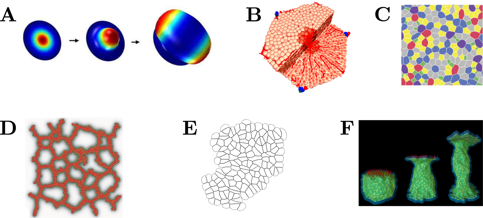
Figure 1.
Tissue and Cell Models. (A) Continuous tissue model of a single cell layer to simulate tip growth and branching, where the surface is displaced in normal direction according to the local signal concentration (reprinted with permission from [6]); (B) Spheroid model of a liver lobule (reprinted with permission from [7]); (C) Vertex model to study epithelial dynamics (reprinted by permission of Elsevier from [8]); (D) Cellular Potts model of blood vessel growth (reprinted with permission from [9]); (E) Immersed Boundary cell model of a proliferating tissue; (F) Subcellular Element model of a single cell subject to a stretching force (reproduced by permission of IOP Publishing from [10]).

Figure 2.
Scales and modelling approaches of signalling (Grey) and tissue modelling approaches (Red). On the horizontal axis, typical length scales are given. The vertical axis indicates increasing computational complexity.
Figure 2.
Scales and modelling approaches of signalling (Grey) and tissue modelling approaches (Red). On the horizontal axis, typical length scales are given. The vertical axis indicates increasing computational complexity.

© 2015 by the authors; licensee MDPI, Basel, Switzerland This article is an open access article distributed under the terms and conditions of the Creative Commons Attribution license (http://creativecommons.org/licenses/by/4.0/).
Share and Cite
MDPI and ACS Style
Tanaka, S. Simulation Frameworks for Morphogenetic Problems. Computation 2015, 3, 197-221. https://doi.org/10.3390/computation3020197
AMA Style
Tanaka S. Simulation Frameworks for Morphogenetic Problems. Computation. 2015; 3(2):197-221. https://doi.org/10.3390/computation3020197
Chicago/Turabian StyleTanaka, Simon. 2015. "Simulation Frameworks for Morphogenetic Problems" Computation 3, no. 2: 197-221. https://doi.org/10.3390/computation3020197