Deformable Cell Model of Tissue Growth

1
Institute of Problems of Mechanical Engineering, Russian Academy of Sciences, 199178 Saint Petersburg, Russia
2
Institut Camille Jordan, UMR 5208 CNRS, University Lyon 1, 69622 Villeurbanne, France
*
Author to whom correspondence should be addressed.
Computation 2017, 5(4), 45; https://doi.org/10.3390/computation5040045
Submission received: 30 September 2017
/
Revised: 24 October 2017
/
Accepted: 24 October 2017
/
Published: 30 October 2017
(This article belongs to the Section Computational Biology)
Abstract
:This paper is devoted to modelling tissue growth with a deformable cell model. Each cell represents a polygon with particles located at its vertices. Stretching, bending and pressure forces act on particles and determine their displacement. Pressure-dependent cell proliferation is considered. Various patterns of growing tissue are observed. An application of the model to tissue regeneration is illustrated. Approximate analytical models of tissue growth are developed.
1. Introduction
Mathematical and computer modelling of tissue growth is used in various biological problems such as wound healing and regeneration, morphogenesis, tumor growth, etc. Tissue growth can be described with continuous models: partial differentiation equations for cell concentrations (reaction–diffusion equations), Navier–Stokes or Darcy equations for the velocity of the medium, and elasticity equations for the distribution of mechanical stresses. There is a vast literature devoted to these models (see, e.g., [1,2,3,4,5] and references therein). Another approach deals with individual-based models where cells are considered as individual objects. It allows a more detailed description at the level of individual cells though analytical investigation of such models becomes impossible and their numerical simulations are often more involved than for the continuous models. There are various lattice and off-lattice cell-based models which can be regrouped as spherical particle models, cellular automata and deformable cell models.
Spherical particle models originate from molecular dynamics. Each cell is considered as a sphere which can interact with the surrounding cells. The force acting between them depends on the distance between their centers. Additional random and dissipative forces can be introduced, as is the case in dissipative particle dynamics [6]. The motion of particles is determined by Newton’s second law. Moreover, cells can divide, die and change their type. Different cell types can have different behavior from the point of view of their motion, division, and death. Already in the 1980s, a similar model, with the equation of motion replaced by some algorithm of cell displacement, was used to study embryogenesis [7]. The spherical particle method to model morphogenesis was developed in a recent work [8]. In [9], one-cell layered tissues were studied under the assumption that there were additional adhesion forces between cells. Hematopoiesis and leukemia development were investigated in [10,11,12,13]. Consecutive cell proliferation and differentiation allowed the description of normal and leukemic hematopoiesis in the bone marrow. Dynamics of cell populations and the conditions of leukemia development were studied. In more complex models, cells can be represented as two connected spherical particles [14].
In the cell-center models, cells are considered as polygons with their centers connected by springs, and cell shape determined by Voronoi tessellation. This approach was used for crypt modelling in [15,16] and brain cancer in [17,18]. Particle models can be combined with continuous models, ordinary and partial differential equations for various intracellular and extracellular concentrations. This hybrid method was used for modelling of cancer [19,20], hematopoiesis and blood diseases [21,22,23,24] and blood clotting in flow [25,26]. In some cases, it is possible to justify transition from particle models to continuous models [27,28,29].
Another approach to tissue growth is based on cellular automata (see [5,30,31] and references therein). This method can be easier to implement and it is better adapted for the transition from discrete to continuous models. On the other hand, it imposes a square lattice geometry which can influence the results. This method is used to study tumor growth [32,33] and cell invasion [34,35], angiogenesis [36,37], tissue engineering [38], and development of avian gut tissue [39]. This approach was further developed in the cellular Potts model [30,40] (see also [41,42] and references therein).
Deformable cell models take into account cell geometry and possible deformation due to mechanical forces. The cell membrane can be considered as an ensemble of particles with various forces acting on them (Section 2). This approach is developed for modeling blood flows where blood cells are considered as individual objects (see [43] and references therein). It is close to the spherical particle models though the particles here do not correspond to individual cells. This method gives more detailed information about cell geometry, adhesion and deformation but it is more difficult to realize, especially in the case of cell division (not considered in the works on blood flows). The questions about the direction of cell division and the mechanical properties of the cell wall become of primary importance here. If they are not sufficiently well described, then the model will fail because of geometrical constraints or because of an accumulation of mechanical stresses.
There are various realizations of the deformable cell model, including the immersed boundary method [44], the subcellular element method [45], and the level set method [46] (see [30] and references therein). The deformable cell model coupled with Navier–Stokes equations was used to study the development of epithelial acini [47,48] and ductal tumor [49]. The interaction of cell geometry and migration for the development of cancer was studied in [50]. A phase field model for collective cell migration was developed in [51]. Deformable cell models for plant growth were developed in [52,53]. Growing shoots and roots have a particular cell organization where dividing cells are located in outer layers of the meristem. Differentiated cells do not divide. The direction of cell division depends on cell location. A precise description of the location of dividing cells and of the direction of their division allowed us to reproduce a self-similar growing structure of the plant root [52]. Directions of cell division and visco-elasto-plastic properties of cell walls are important in modelling root growth with a deformable cell model.
In this work, we continue to develop the deformable cell model of tissue growth. The main assumptions of the model are similar to those in [52] except for the location of dividing cells and the direction of their division. Instead of a particular cell structure and division specific for root and shoot meristem, we consider uniform tissue growth where dividing cells can be located everywhere. The direction of their division is determined by a special algorithm described in the next section. We will describe the deformable cell model in Section 2. Some properties of growing tissues and applications are discussed in Section 3. Section 4 is devoted to an approximate analytical model of tissue growth.
2. Deformable Cell Model
2.1. Forces
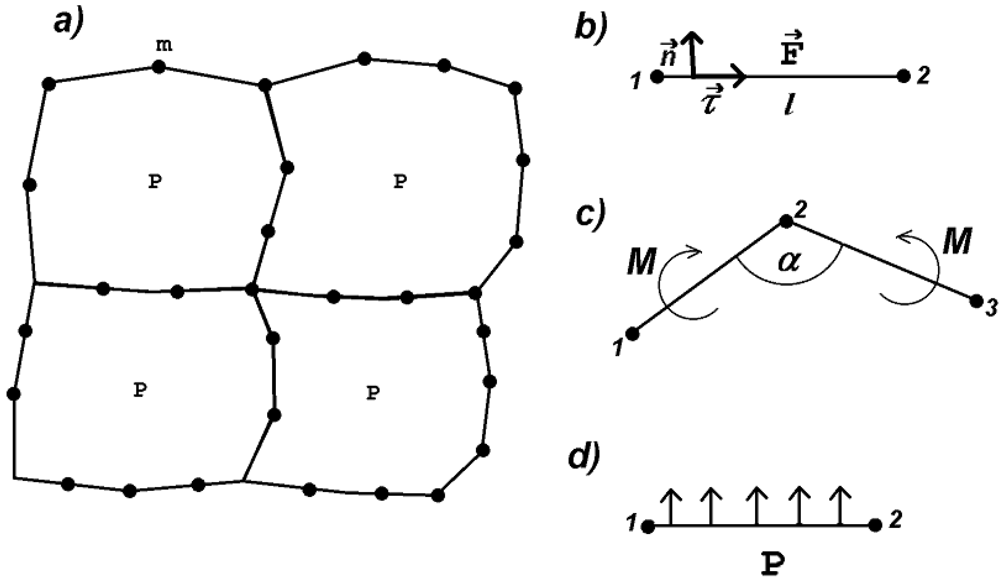
We begin the description of the model with mechanical forces acting in cellular structures. An individual cell at its mechanical equilibrium (without deformation) represents a regular polygon with n vertices. Initially, it has an area , the length of the sides and the angle between any neighboring sides . These parameters can be different for different cells. We place a particle of mass m at each vertex of the polygon.
If the polygon changes its shape, then there are three forces which tend to return it to its original configuration. They depend on the change of side length, angles and volume. Similar to other deformable cell models, we define them as follows. If the length l of a side changes, then there is a force acting on each of the two vertices located at this side:
(Figure 1b). Here, is the unit vector along the side. If the angle between two sides changes (Figure 1c), then there is momentum
which creates a pair of forces applied to the vertices and acting on each side in the direction perpendicular to it, . Finally, if the cell area S changes, then there is a force (pressure)
applied to each side and acting in the direction perpendicular to it (Figure 1d). Let us note that the first terms in (1)–(3) describe elastic force and the second term viscous dissipation. They correspond to visco-elastic properties of biological cells. The problem is considered in dimensionless variables. Coefficients are material parameters which determine the resistance to stretching, bending and compression. Parameters represent artificial viscosity introduced in order to avoid numerical instability.
The total force acting on the i-th vertex is a sum of these three forces. The position of this vertex is determined by the equations
where is the vertex velocity, is the coefficient which determines viscous friction from the surrounding medium.
For further description of the model, we denote by the side length at mechanical equilibrium and by l its length in the process of cell growth and deformation. Due to plastic deformations, can change. So, we will distinguish the initial value which corresponds to the moment of cell appearance, and the current value , which can be different from . We introduce two additional features in the model:
- If the length of a side becomes twice as large as its initial length , then an additional vertex is introduced in the middle of the side. At the moment of side division, the stretching force is preserved. Hence the number of vertices depends on cell deformation. This allows us to better describe cell shape in the case of large deformations.
- If the length l of a side becomes sufficiently large, that is , with some , , then the initial length increases irreversibly in such a way that it satisfies the equality . In this case, if the stretching force is removed, then the spring will not return to its initial length but to some greater length. This corresponds to the irreversible deformation of the cell wall when it grows. Here, is a material parameter characterizing plastic deformation observed for biological tissues. In the simulations presented below, we set .
2.2. Cell Growth and Division
2.2.1. Cell Growth
The cell area (without deformation) of growing cells changes in time with the rate:
where is some given function. We set , if a cell does not grow and const in the case of linear growth. Other growth rates can also be considered [52]. When increases two-fold, the cell divides. The area of the daughter cell (without deformation) returns to the two-fold lower value. When studying root growth, we also introduced cell growth without division [52].
2.2.2. Cell Division
One of the important characteristics of growing tissue is the directions of cell division. If these directions are not coordinated, then cells can become strongly deformed. This contradicts biological observations and can result in failure of the numerical method. We will choose the direction of cell division according to the algorithm explained below. This algorithm is specific for unpolarized cells [47].
Let us recall that cells are represented as polygons. They grow, increasing their volume, and divide into two cells with approximately equal areas. Cell division occurs along a section connected to vertices (diagonal) of the polygon. Only such sections are considered. For each cell, the algorithm of choice of the section consists of two steps. In the first step, we choose all sections which divide the polygon into two parts with approximately equal area. Since these two areas are determined by the vertices of the polygon, in general they are not exactly equal to each other. Therefore, we introduce a maximal possible difference . Hence we choose all sections such that the areas and of two resulting post-division polygons satisfy the condition . Here, . In the second step of the algorithm, we choose the shortest section among all of those chosen in the first step. Let us note that this algorithm depends on the location of cell nodes.
Thus, we can summarize this algorithm as a choice of the shortest section by dividing the polygon into two subpolygons with approximately equal areas. Due to this algorithm of cell division, cells cannot be strongly deformed (elongated). We will see that it provides stable tissue growth in a wide range of parameters. Other approaches to the direction of cell division were used in [52] in order to model plant root growth and other polarized cells in [47].
3. Numerical Modelling of Tissue Growth
3.1. All Cells Grow and Divide
Modelling of tissue growth with a deformable cell model implies certain restrictions on the location of dividing cells and on the direction of their division. If these condition are not satisfied, then it will lead to a rapid accumulation of mechanical stresses and to failure of the cellular structure. One possible cell organization was suggested in [52] for the description of root growth. According to the biological observations, dividing cells are located in this case close to the outer surface of the growing root. Directions of cell division are also precisely determined. In this work, we consider a uniform tissue growth where all cells of the tissue can divide.
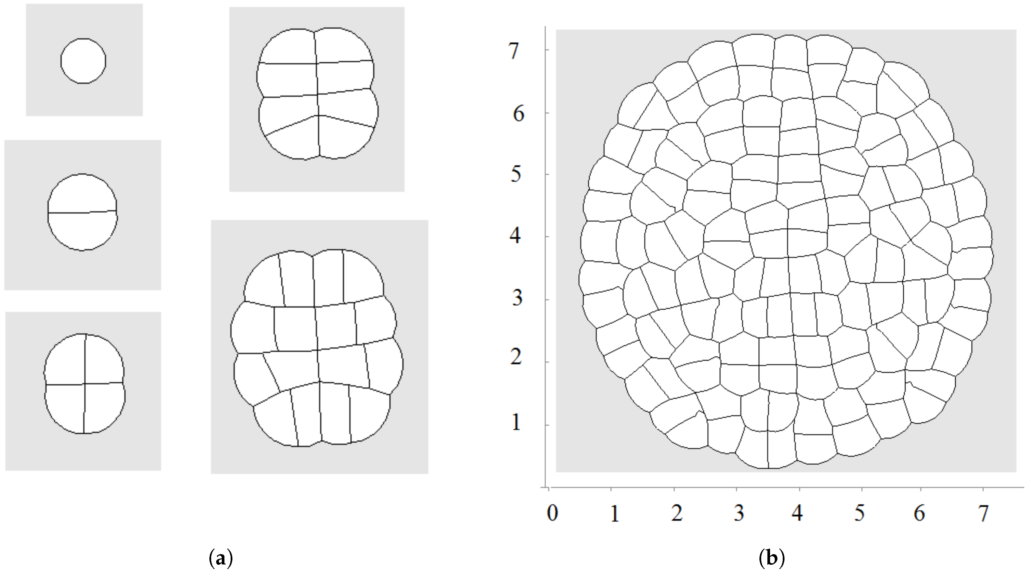
Let us recall that each cell is characterized by its equilibrium area and current area S. The equilibrium area grows here as a linear function of time. An example of a growing tissue is shown in Figure 2. Each cell grows and divides. The direction of division is determined by the shortest diagonal algorithm described above. Initially, there are 20 nodes at the surface of the cell in this simulation. Other nodes can be added if the distance between two neighboring nodes exceeds some given value. We will use the values of parameters , , (time step), , , unless other values are specified.
The first division occurs along a diameter of the circular cell. The second division takes place along the perpendicular diameter. These first two divisions form the axis of the growing cell structure. They determine the next several divisions. However, during further growth of the tissue, the axes are not preserved and radial structure begins to emerge. The outer cells divide either in the direction parallel to the outer surface or perpendicular to it. This cell organization becomes more obvious during further growth (Figure 3 and Figure 4a). Let us also note that the shapes of the cells represent mostly polygons with four or five vertices. The cell structure symmetry is lost after several divisions because cells have approximately equal area but not exactly equal. Therefore, even after the first division, the two daughter cells are slightly different.
3.2. Pressure-Dependent Proliferation
Cell division leads to cells’ compression and to internal pressure growth. Initially, internal pressure in a separate cell equals zero because the cell has its equilibrium shape. When it grows, its equilibrium area increases linearly in time. Its actual area also grows but slower because the cell membrane resists elongation. This difference creates internal cell pressure. When the cell divides, its equilibrium area is divided by 2 and its actual area is divided approximately by 2. Therefore, the value of pressure remains approximately the same. Moreover, since cells are attached to each other, they cannot return to the circular shape for which the area is maximal. Cell deformation increases the pressure.
Maximal pressure (among all cells) is reached at the center of the domain filled by cells. It grows exponentially in time (Figure 5a) because cells at the center need to push surrounding cells more and more in order to expand. This is related to the exponential growth of cell number (Section 4). For a fixed time, the maximal pressure depends on parameters. It grows approximately as a linear function of viscosity (Figure 5b). It can be compared with fluid flow in a porous medium where pressure difference is proportional to the viscosity (Section 4).
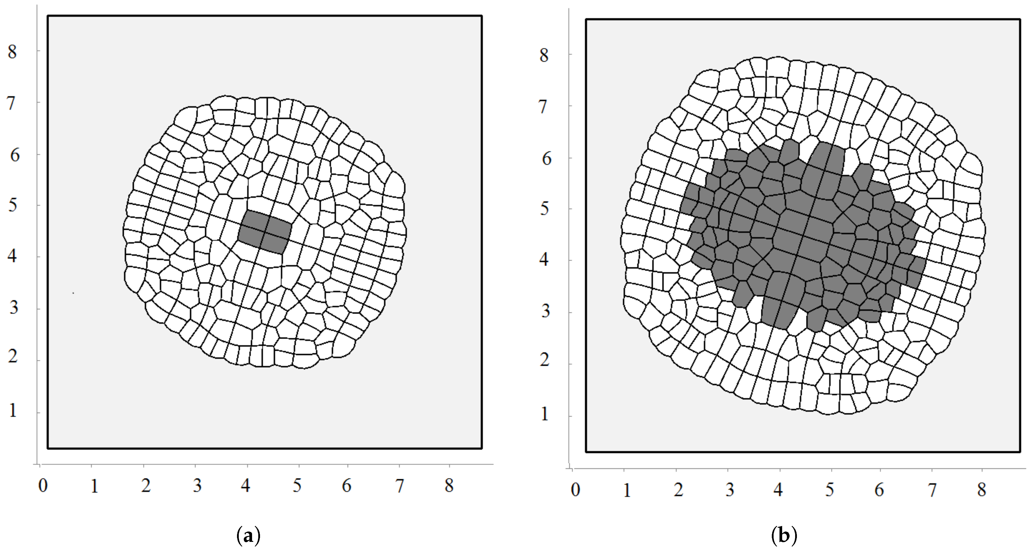
Biological cells cannot divide when they are too compressed (see [54] and references therein). In order to describe this effect, we introduce the maximal pressure beyond which cells do not divide. Let us recall that pressure P inside cells is determined by Equation (3). We impose an additional condition that if P is greater than some critical value , then the cell does not divide. Figure 4a shows a snapshot of the growing cells’ structure for the maximal division pressure . We obtain a regular structure close to a circle with radial cell organization near its outer border. Cells there divide either in the direction parallel to the boundary or perpendicular to it. The latter increases the number of cells in the outer layer and provides growth of the perimeter. Similar cell structures can be observed in the cross-section of growing plant branches.
The value of the maximal division pressure can influence the properties of the growing cell structure. Another example is shown in Figure 4b. Here, the maximal division pressure is set at after a short initial period when (otherwise, the first divisions do not occur). In this case, there are cells which do not divide even at the outer surface. This results in the appearance of the specific asymmetric structure with a curved surface and “leaves” separated by an interface. Cells at the interface do not divide since the pressure there is greater than the critical value .
The appearance of curved structures can be considered as instability of symmetric circular structures. This instability results from cell competition for space. More compressed cells do not grow, and less compressed cells grow and take even more space. As happens in many other examples, the instability occurs near the extinction limit where the cell structure stops growing because of the excessively high pressure.
We consider one more example where cells die by apoptosis if they do not divide during some time. This is related to the check points during the cell cycle. In this case, they are removed from the computational domain. In this case, there is a curved front of cells slowly propagating outwards and numerous cell clusters inside (Figure 4c). This is a non-stationary structure where cells divide and expand if they have enough space; they stop dividing and disappear if there is not enough space.
3.3. External Supply of Nutrients
If nutrients come from outside of the growing tissue, as is the case for tumor growth, then exterior cells have more nutrients than the cells inside the tissue. They will grow and divide faster than cells inside the tissue. They will also compete for nutrients. This competition can lead to nonuniform tissue growth and to the emergence of asymmetric structures. This effect was also observed in hybrid models of tumor growth [55].
In this section, we illustrate it with the deformable cell model. We assume that the growth rate of exterior cells is proportional to the length of their exterior boundary. This assumption implies that the concentration of nutrients in the medium surrounding the tissue is constant and their consumption by cells is proportional to the length of the cell boundary.
If we assume that nutrients can be transported inside the tissue, then interior cells will also have some nutrients. In order to simplify the model, we will suppose that the concentration of nutrients in the extracellular matrix at some point inside the tissue is the same as in the cell located at this point. The flux of nutrients q between cells is proportional to the difference of concentrations and in the neighboring cells and to the length L of the boundary between them, . Here, is a parameter which determines the flux intensity.
Figure 6 shows examples of numerical simulations of tissue growth with an external supply of nutrients only to the outer cells and to the interior cells in the case of nutrient diffusion in the tissue. We observe asymmetric growth which results from cell competition for nutrients. A cell which has a longer exterior boundary will grow and divide faster and will compress surrounding cells, reducing their exterior boundary and growth rate. Moreover, the pressure-dependent proliferation increases this competition because compressed cells can stop their growth completely. Emerging structures are more pronounced here than in the model without nutrients (Section 3.2).
3.4. Wound Healing
Together with tumor growth, wound healing is one of the main applications of tissue growth models. An extensive literature review on this subject can be found in [56]. A conventional approach to study wound healing consists in the analysis of travelling wave solutions of the reaction–diffusion system of equations for the cell density and for the concentration of some substances which influence cell proliferation (e.g., oxygen). The wave of cell proliferation fills the spatial domain, which corresponds to the wound and which is surrounded by the remaining tissue. In this section, we illustrate modelling of wound healing with the deformable cell model. We will see that pressure-dependent proliferation is an appropriate mechanism to control wound closure.
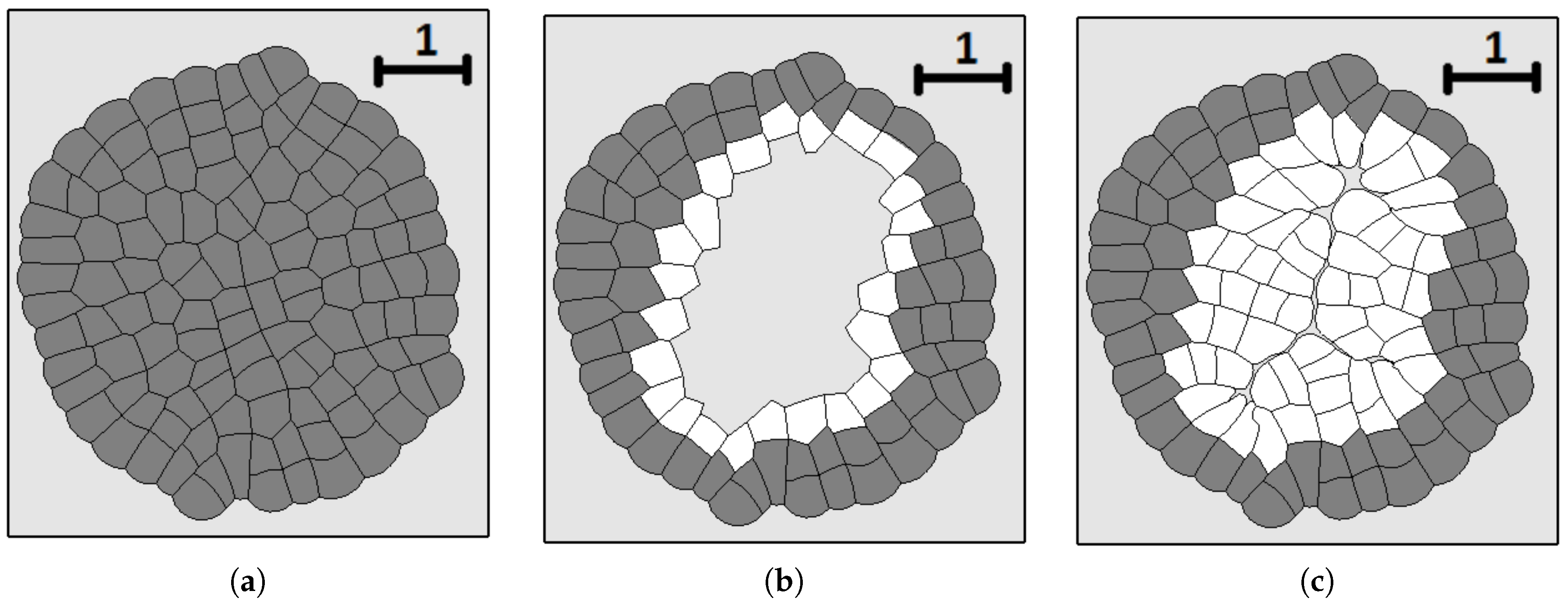
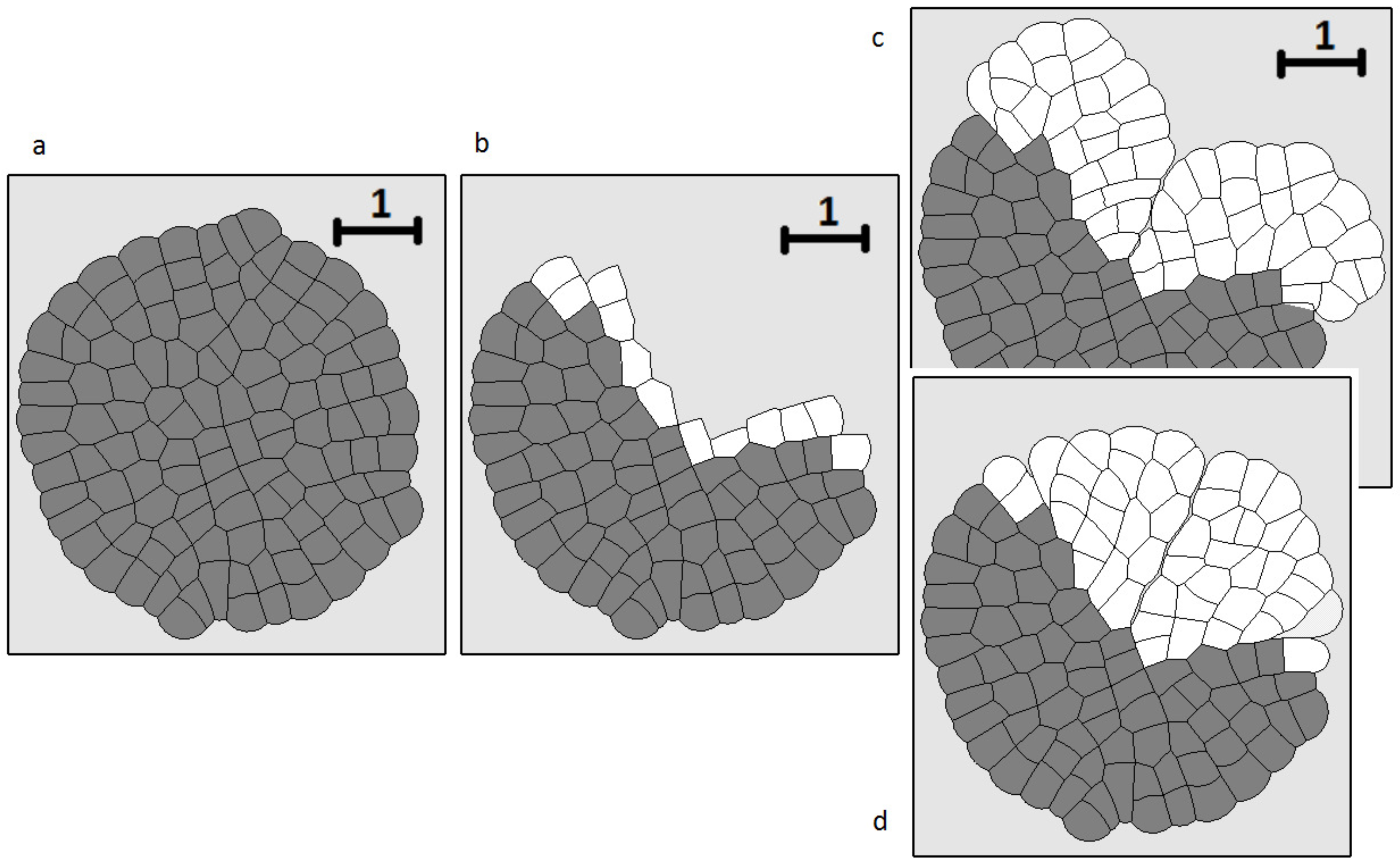
Figure 7 shows an example of numerical simulations of tissue regeneration. The original tissue (left image) is obtained from a single cell as described above. The cells of this tissue are fixed—they do not grow or divide any more. After that, we remove the internal part of the tissue. The cells at the boundary of the removed tissue can grow and divide. They fill the available place. They stop growing and divide when the tissue is regenerated due to pressure-dependent proliferation. Cells push each other, internal pressure grows and they no longer grow and divide. The new tissue fits the form of the wound well. However, some damage remains at the place where two parts of the tissue meet each other. Its size depends on the mechanical properties of cells. It decreases if cells are more deformable and better fit each other.
Another example of tissue regeneration is shown in Figure 8. The main difference here in comparison with the previous example is that the region where a part of the tissue is removed is not bounded by the remaining tissue (Figure 8b). If we use the same approach as in the previous case, we obtain a different form of the regenerated tissue compared with the initial tissue (Figure 8c). In order to reproduce the form of the original tissue, we need to introduce different growth rates for different cells. Consider cells located at the wound surface in Figure 8b. We impose a particular growth rate for each of these cells. Their descendants will preserve these growth rates. The cells located closer to the outer surface grow and divide slowly. The growth rate and division increase as much as the cells go deeper into the damaged tissue. The maximal growth rate is reached at the center. Such distribution of the growth rate allows us to approximate the initial tissue form by the regenerated tissue (Figure 8d). It should also be noted that this tissue continues to grow even when the initial form is regenerated. Therefore, there are additional mechanisms which control the size of the tissue [57,58,59].
Let us note that if the critical value is high enough, it will not influence cell division. On the other hand, there is a biochemical regulation of the cell division rate, implying that some cells divide faster than others. This regulation is not explicitly introduced in the model but it acts implicitly through the cell location.
4. Analytical Approximation of the Growth Rate
4.1. Approximate Model
Passing from the equation of motion of individual particles to an approximate averaged equation of motion of the medium, we get
where v is the velocity of the medium and p is the pressure (see [27] for more detail). We consider this equation in the one-dimensional case in order to obtain an approximate analytical solution. It corresponds to the two-dimensional case with plane geometry or to the circular tissue with a sufficiently large radius. Equation (5) is a macroscopic analogue of Equation (4) with an average force proportional to the pressure gradient. It should be noted, however, that force in (4) also contains other components. So, the analytical continuous model is an approximation. Parameter in both equations corresponds to viscous friction.
We will consider this equation in the quasi-stationary approximation,
which takes the form of the Darcy equation for the porous medium. Next, we will assume that the medium is incompressible. This assumption is justified for sufficiently large values of the pressure force coefficient in the cell model. In this case, cells preserve their volume and, in the limit of large coefficients, the medium becomes incompressible. In this case, the mass conservation (or continuity) equation can be written as follows:
where W is the rate of production of mass. In the one-dimensional case, divergence is the space derivative . Production of mass is determined by the rate of cell division . We will suppose that it depends on the pressure. When biological cells are strongly compressed, they do not divide. This assumption is consistent with pressure-dependent proliferation in the cell model (Section 3), which can be considered as discretization of the continuous model.
4.2. Constant Proliferation
If the proliferation rate does not depend on pressure, then we set , where b is some positive constant. We solve Equation (8) in the interval with the boundary condition . We obtain
Since , then taking into account (6), we have
Hence the length of the interval grows exponentially. If we consider a circular tissue with the radius , then neglecting the influence of the curvature on the growth rate, we get the formula for the tissue area :
where is the initial area.
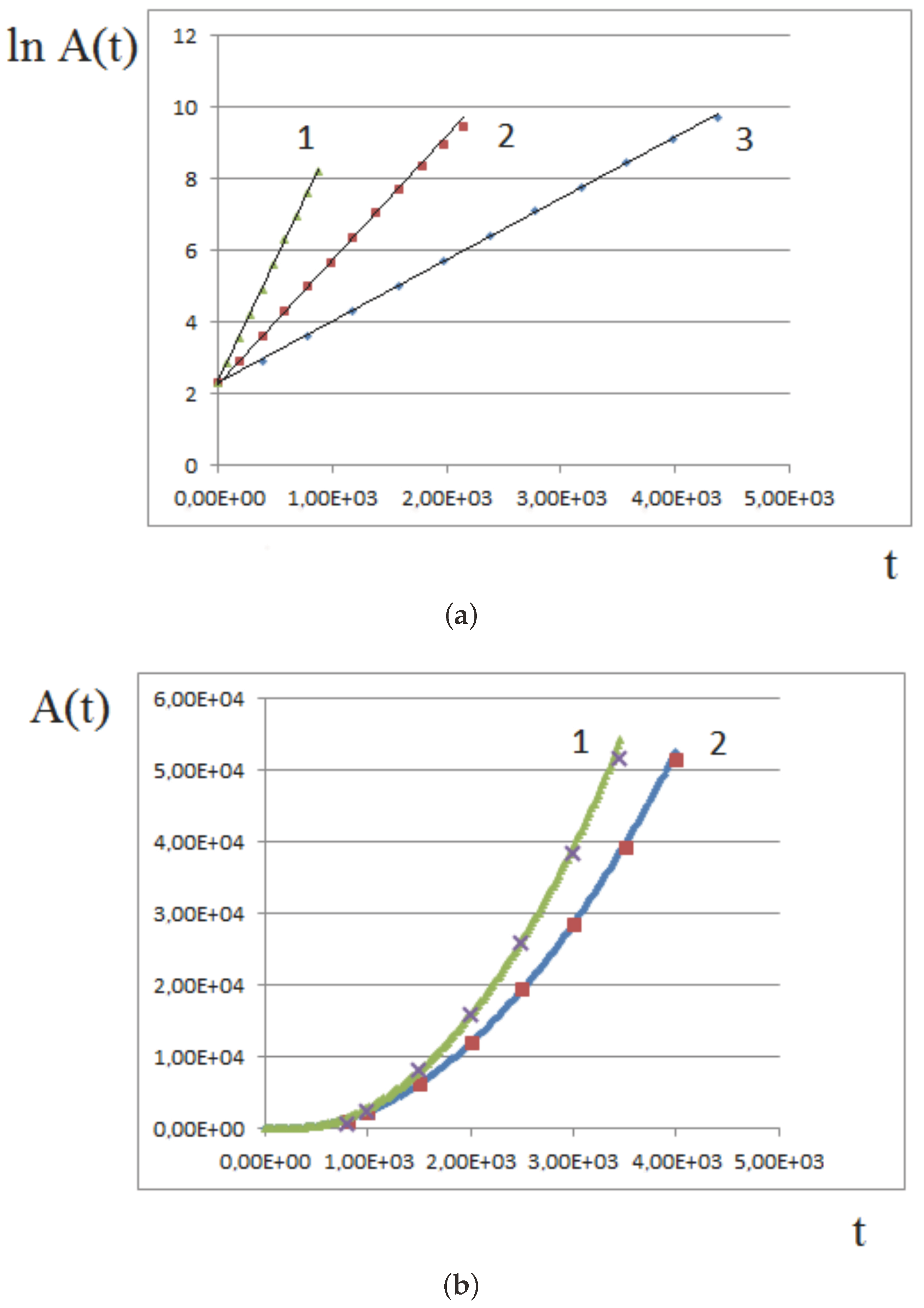
Figure 9a shows an example of numerical simulations of tissue growth with a constant proliferation rate. The linear dependence of the logarithm of tissue area on time, , shows that the growth rate is exponential. Three different proliferation rates are considered, . The slopes of the straight lines are in the same proportions. For large amounts of time, the assumptions of the model may not be satisfied, and the growth rate slows down in comparison with the exponential one.
4.3. Pressure-Dependent Proliferation
We will consider a piece-wise constant function :
Let us suppose that the medium fills the half-axis . We should complete the formulation of the problem by the boundary condition for the pressure
where is some non-negative constant, .
We can now solve problem (8) and (9). Suppose that the value is reached at . Taking into account the continuity of pressure and of its first derivative at , we obtain
where . From the boundary condition (9), we find the value of :
Hence
In the case of circular tissue growth, neglecting curvature, we can approximate the growth rate of irs radius R by the formula
Hence we obtain the formula for the tissue area :
Figure 9b shows the results of numerical simulations of tissue growth and comparison with the analytical approximation. At the beginning of growth, when the pressure-dependent proliferation is not yet established, all cells divide, and the growth rate is exponential. Therefore, instead of Formula (10), we approximate it by the expression
where the coefficients a and b are chosen to fit the simulations presented in Section 3.1 with two different values of maximal pressure: and . The curves are well approximated by Formula (11) with and .
In order to compare more precisely the values of a obtained in numerical simulations with the coefficient
in (10), we need to specify the value of pressure at the boundary. This is the pressure in the cells at the outer layer. It varies during cell growth. Its average value depends on the values of parameters. For the basic set of parameters, . Hence the right-hand side in (12) increases twice when we compare and while the coefficient a on the left-hand side obtained from numerical simulations in times. This difference is related to the fact that intracellular pressure in the numerical model (Section 3) is only a part of the total pressure in the analytical model. The latter also takes into account the contribution from elastic forces.
If we decrease the value of the stretching coefficient, (instead of above), then pressure in cells at the outer layer decreases. Therefore, growth accelerates and we get . This example shows how mechanical properties of cells influence the growth rate of the tissue and how they influence macroscopic phenomenological parameters.
5. Discussion
In this work, we developed a deformable cell model of growing tissue where cells are attached to each other. Two neighboring cells have the same boundary and cannot be separated. Another possible approach is to consider separated cells which can adhere due to additional forces acting between them [47,48]. The direction of cell division is chosen along the shortest diagonal which divides the cell into two cells with approximately equal areas. This algorithm appears to be very robust and allows us to simulate tissue growth with more than cells. Pressure-dependent proliferation, which corresponds to biological observations, can result in the appearance of asymmetric tissue structures.
The spring model of cells (Section 2) can be considered as an approximation of an elastic medium. Together with viscosity in the equation for particle displacement, we obtain a viscoelastic medium. Using the porous medium equation to describe it, we simplify the model but we obtain a good approximation of the tissue growth rate.
Modelling of tissue growth with the deformable cell model can be applied to study tumor growth. In the case of pressure-dependent proliferation, it describes the linear growth rate of the tissue radius specific for tumors after a short initial stage of exponential growth [54]. The growing tumor can lose its radial symmetry, resulting in the appearance of spatial structures. This instability can be related to cell competition for nutrients, and it can be modeled with partial differential equations [60,61,62,63,64] or with cell-based models [32,55] (see also references in [54]). However, as is indicated in [54], in vitro experiments show a smoother shape of the growing tumor. It is suggested that another possible mechanism of pattern formation can be related to mechanical stresses: cells diffuse along the surface searching for a free space. Results presented in this work show that indeed, competition for nutrients is not the only possible mechanism of instability. Mechanical constraints lead to the emergence of spatial structures. The introduction of nutrients increases their roughness. Hence pressure-dependent proliferation, a linear growth rate (exponential rate at the beginning) and various mechanisms of pattern formation of growing tissues observed in numerical simulations are in agreement with the experiments in vitro.
Another classic example of tissue growth is wound healing. It is conventionally modelled with reaction–diffusion equations for the concentrations of cells and some substances which determine their proliferation. A wave of cell proliferation propagates in the wound region and fills it. The deformable cell model of tissue growth is an appropriate tool to study wound healing. Even without additional concentrations, pressure-dependent proliferation allows us to control wound closure. When two borders of the wound meet and cells touch each other, their proliferation stops. However, if we consider the wound cross-section perpendicular to the epidermis, the wound area is not bounded by the remaining tissue from one side. Therefore, the problem here is different: how to control the form and the size of the growing tissue in an open domain. In this case, we need to introduce the rate of cell proliferation which depends on its position. This question requires further investigation.
The model presented in this work has certain limitations. First of all, we consider a two-dimensional tissue (cell sheet) while most biological tissues are essentially three-dimensional. Numerical simulations in this case become more involved but we expect that the main properties discussed above remain the same. Cell division and death are determined by the intracellular and extracellular regulations which can be described by ordinary or partial differential equations. Such hybrid discrete-continuous models [65] are used in the case of a simplified cell representation (e.g., soft sphere model) but not for the deformable cell models. Let us also note that mechanical properties of the tissue can influence molecular transport [66] and, consequently, cell fate. Mechanical forces can influence cell division and migration [67]. These and other questions require further investigation and the development of more specific models.
Author Contributions
N.B. developed computational software and V.V. performed the simulations. N.B. and V.V. wrote the paper.
Conflicts of Interest
The authors declare no conflicts of interest.
References
- Basan, M.; Elgeti, J.; Hannezo, M.; Rappel, W.-J.; Levine, H. Alignment of cellular motility forces with tissue flow as a mechanism for efficient wound healing. Proc. Natl. Acad. Sci. USA 2013, 110, 2452–2459. [Google Scholar] [CrossRef] [PubMed] [Green Version]
- Chauviere, A.; Preziozi, L.; Verdier, C. (Eds.) Cell Mechanics: From Single Cell-Based Models to Multi-Scale Modeling; CRC Press: London, UK, 2010. [Google Scholar]
- Friedman, A. (Ed.) Tutorials in Mathematical Biosciences III; Cell Cycle, Proliferation, and Cancer; Springer: Berlin, Germany, 2006. [Google Scholar]
- Capasso, V.; Gromov, M.; Harel-Bellan, A.; Morozova, N.; Pritchard, L. (Eds.) Pattern Formation in Morphogenesis. In Springer Proceedings in Mathematics; Springer: Berlin, Germany, 2012; Volume 15. [Google Scholar]
- Glade, N.; Stephanou, A. (Eds.) Le Vivant Entre Discret et Continu; Editions Matériologiques: Paris, France, 2013. [Google Scholar]
- Karttunen, M.; Vattulainen, I.; Lukkarinen, A. A Novel Methods in Soft Matter Simulations; Springer: Berlin, Germany, 2004. [Google Scholar]
- Bodenstein, L. A dynamic simulation model of tissue growth and cell patterning. Cell Differ. 1986, 19, 19–33. [Google Scholar] [CrossRef]
- Markov, M.A.; Markov, A.V. Computer simulation of the ontogeny of organisms with different types of symmetry. Paleontol. J. 2014, 48, 1–9. [Google Scholar] [CrossRef]
- Drasdo, D.; Loeffler, M. Individual-based models to growth and folding in one-layered tissues: Intestinal crypts and early development. Nonlinear Anal. 2001, 47, 245–256. [Google Scholar] [CrossRef]
- Bessonov, N.; Pujo-Menjouet, L.; Volpert, V. Cell modelling of hematopoiesis. Math. Model. Nat. Phenom. 2006, 1, 81–103. [Google Scholar] [CrossRef]
- Bessonov, N.; Demin, I.; Pujo-Menjouet, L.; Volpert, V. A multi-agent model describing self-renewal or differentiation effect of blood cell population. Math. Comput. Model. 2009, 49, 2116–2127. [Google Scholar] [CrossRef]
- Bessonov, N.; Crauste, F.; Demin, I.; Volpert, V. Dynamics of erythroid progenitors and erythroleukemia. Math. Model. Nat. Phenom. 2009, 4, 210–232. [Google Scholar] [CrossRef]
- Bessonov, N.; Demin, I.; Kurbatova, P.; Pujo-Menjouet, L.; Volpert, V. Multi-Agent Systems and Blood Cell Formation. In Multi-Agent Systems—Modeling, Interactions, Simulations and Case Studies; Alkhateeb, F., Al Maghayreh, E., Doush, I.A., Eds.; InTech: Rijeka, Croatia, 2011. [Google Scholar]
- Ranfta, J.; Basan, M.; Elgeti, J.; Joanny, J.-F.; Prost, J.; Jülicher, F. Fluidization of tissues by cell division and apoptosis. PNAS 2010, 107, 20863–20868. [Google Scholar] [CrossRef] [PubMed]
- Meineke, F.A.; Potten, C.S.; Loeffer, M. Cell migration and organization in the intestinal crypt using a lattice-free model. Cell Prolif. 2001, 34, 253–266. [Google Scholar] [CrossRef] [PubMed]
- Van Leeuwen, I.M.; Mirams, G.R.; Walter, A.; Fletcher, A.; Murray, P.; Osborne, J.; Varma, S.; Young, S.J.; Cooper, J.; Doyle, B.; et al. An integrative computational model for intestinal tissue renewal. Cell Prolif. 2009, 42, 617–636. [Google Scholar] [CrossRef] [PubMed]
- Kansal, A.R.; Torquato, S.; Harsh, G.R.; Ciccaeb, E.A.; Deisboeck, T.S. Simulated Brain Tumor Growth Dynamics Using a Three-Dimensional Cellular Automaton. J. Theor. Biol. 2000, 203, 367–382. [Google Scholar] [CrossRef] [PubMed]
- Kansal, A.R.; Torquato, S.; Harsh, G.R.; Chiocca, E.A.; Deisboeck, T.S. Cellular automaton of idealized brain tumor growth dynamics. BioSystems 2000, 55, 119–127. [Google Scholar] [CrossRef]
- Ramis-Conde, I.; Drasdo, D.; Anderson, A.R.A.; Chaplain, M.A.J. Modeling the Influence of the E-Cadherin-b-Catenin Pathway in Cancer Cell Invasion: A Multiscale Approach. Biophys. J. 2008, 95, 155–165. [Google Scholar] [CrossRef] [PubMed]
- Ramis-Conde, I.; Chaplain, M.A.J.; Anderson, A.R.A.; Drasdo, D. Multi-scale modelling of cancer cell intravasation: The role of cadherins in metastasis. Phys. Biol. 2009, 6, 016008. [Google Scholar] [CrossRef] [PubMed]
- Bessonov, N.; Eymard, N.; Kurbatova, P.; Volpert, V. Mathematical modelling of erythropoiesis in vivo with multiple erythroblastic islands. Appl. Math. Lett. 2012, 25, 1217–1221. [Google Scholar] [CrossRef]
- Eymard, N.; Bessonov, N.; Gandrillon, O.; Koury, M.J.; Volpert, V. The role of spatial organization of cells in erythropoiesis. J. Math. Biol. 2015, 70, 71–97. [Google Scholar] [CrossRef] [PubMed]
- Fischer, S.; Kurbatova, P.; Bessonov, N.; Gandrillon, O.; Volpert, V.; Crauste, F. Modelling erythroblastic islands: Using a hybrid model to assess the function of central macrophage. J. Theor. Biol. 2012, 298, 92–106. [Google Scholar] [CrossRef] [PubMed]
- Kurbatova, P.; Eymard, N.; Volpert, V. Hybrid Model of Erythropoiesis. Acta Biotheor. 2013, 61, 305–315. [Google Scholar] [CrossRef] [PubMed]
- Tosenberger, A.; Ataullakhanov, F.; Bessonov, N.; Panteleev, M.; Tokarev, A.; Volpert, V. Modelling of thrombus growth in flow with a DPD-PDE method. J. Theor. Biol. 2013, 337, 30–41. [Google Scholar] [CrossRef] [PubMed]
- Tosenberger, A.; Bessonov, N.; Volpert, V. Influence of fibrinogen deficiency on clot formation in flow by hybrid model. Math. Model. Nat. Phenom. 2015, 10, 36–47. [Google Scholar] [CrossRef] [Green Version]
- Bessonov, N.; Kurbatova, P.; Volpert, V. Particle dynamics modelling of cell populations. Math. Model. Nat. Phenom. 2010, 5, 42–47. [Google Scholar] [CrossRef]
- Colombi, A.; Scianna, M.; Preziosi, L. A measure-theoretic model for collective cell migration and aggregation. Math. Model. Nat. Phenom. 2015, 10, 4–35. [Google Scholar] [CrossRef]
- Kurbatova, P.; Panasenko, G.; Volpert, V. Asymptotic numerical analysis of the diffusion-discrete absorption equation. Math. Methods Appl. Sci. 2012, 35, 438–444. [Google Scholar] [CrossRef]
- Anderson, A.R.A.; Chaplain, M.; Rejniak, K.A. Single Cell Based Models in Biology and Medicine; Birkhäuser: Basel, Switzerland, 2007. [Google Scholar]
- Deutsch, A.; Dormann, S. Cellular Automaton Modeling of Biological Pattern Formation; Birkhäuser: Boston, MA, USA, 2005. [Google Scholar]
- Gerlee, P.; Anderson, A.R.A. A hybrid cellular automaton model of clonal evolution in cancer: The emergence of the glycolytic phenotype. J. Theor. Biol. 2008, 250, 705–722. [Google Scholar] [CrossRef] [PubMed]
- Patel, A.A.; Gawlinskia, E.T.; Lemieuxe, S.K.; Gatenby, A.A. A Cellular Automaton Model of Early Tumor Growth and Invasion: The Effects of Native Tissue Vascularity and Increased Anaerobic Tumor Metabolism. J. Theor. Biol. 2001, 213, 315–331. [Google Scholar] [CrossRef] [PubMed]
- Simpson, M.J.; Merrifield, A.; Landman, K.A.; Hughes, B.D. Simulating invasion with cellular automata: Connecting cell-scale and population-scale properties. Phys. Rev. E 2007, 76, 021918. [Google Scholar] [CrossRef] [PubMed]
- Simpson, M.J.; Landman, K.A.; Hughes, B.D. Distinguishing between Directed and Undirected Cell Motility within an Invading Cell Population. Bull. Math. Biol. 2009, 71, 781–799. [Google Scholar] [CrossRef] [PubMed]
- Anderson, A.R.A.; Rejniak, K.A.; Gerlee, P.; Quaranta, V. Microenvironment driven invasion: A multiscale multimodel investigation. J. Math. Biol. 2009, 58, 579–624. [Google Scholar] [CrossRef] [PubMed]
- Stephanou, A.; McDougall, S.R.; Anderson, A.R.A.; Chaplain, M.A.J. Mathematical modelling of the influence of blood rheological properties upon adaptative tumour-induced angiogenesis. Math. Comput. Model. 2006, 44, 96–123. [Google Scholar] [CrossRef]
- Chung, C.A.; Lin, T.H.; Chen, S.D.; Huang, H.I. Hybrid cellular automaton modeling of nutrient modulated cell growth in tissue engineering constructs. J. Theor. Biol. 2010, 262, 267–278. [Google Scholar] [CrossRef] [PubMed]
- Binder, B.J.; Landman, K.A.; Simpson, M.J. Modeling proliferative tissue growth: A general approach and an avian case study. Phys. Rev. E 2008, 78, 031912. [Google Scholar] [CrossRef] [PubMed]
- Merks, R.M.H.; Glazier, J.A. A cell-centered approach to developmental biology. Phys. A 2005, 352, 113–130. [Google Scholar] [CrossRef]
- Albert, P.J.; Schwarz, U.S. Dynamics of Cell Ensembles on Adhesive Micropatterns: Bridging the Gap between Single Cell Spreading and Collective Cell Migration. PLoS Comput. Biol. 2016. [Google Scholar] [CrossRef] [PubMed] [Green Version]
- Scianna, M.; Preziosi, L. Cellular Potts Models: Multiscale Extensions and Biological Applications; Chapman and Hall: London, UK; CRC: Boca Raton, FL, USA, 2013. [Google Scholar]
- Bessonov, N.; Babushkina, E.; Golovashchenko, S.F.; Tosenberger, A.; Ataullakhanov, F.; Panteleev, M.; Tokarev, A.; Volpert, V. Numerical modelling of cell distribution in blood flow. Math. Model. Nat. Phenom. 2014, 9, 69–84. [Google Scholar] [CrossRef]
- Peskin, C.S. The immersed boundary method. Acta Numer. 2002, 11, 479–517. [Google Scholar] [CrossRef]
- Newman, T.J. Modeling multicellular systems using subcellular elements. Math. Biosci. Eng. 2005, 2, 613–624. [Google Scholar] [CrossRef] [PubMed]
- Koumoutsakos, P.; Bayati, B.; Milde, F.; Tauriello, G. Particle simulations of morphogenesis. Math. Models Methods Appl. Sci. 2011, 21, 955–1006. [Google Scholar] [CrossRef]
- Rejniak, K.A.; Anderson, A.R.A. A Computational Study of the Development of Epithelial Acini: I. Sufficient Conditions for the Formation of a Hollow Structure. Bull. Math. Biol. 2008, 70, 677–712. [Google Scholar] [CrossRef] [PubMed]
- Rejniak, K.A.; Anderson, A.R.A. A Computational Study of the Development of Epithelial Acini: II. Necessary Conditions for Structure and Lumen Stability. Bull. Math. Biol. 2008, 70, 1450–1479. [Google Scholar] [CrossRef] [PubMed]
- Rejniak, K.A.; Dillon, R.H. A single cell based model of the ductal tumour microarchitecture. Comput. Math. Methods Med. 2007, 8, 51–69. [Google Scholar] [CrossRef]
- Tozluoglu, M.; Tournier, A.L.; Jenkins, R.P.; Hooper, S.; Bates, P.A.; Sahai, E. Matrix geometry determines optimal cancer cell migration strategy and modulates response to interventions. Nat. Cell Biol. 2013, 15, 751–762. [Google Scholar] [CrossRef] [PubMed]
- Lober, J.; Ziebert, F.; Aranson, I.S. Collisions of deformable cells lead to collective migration. Sci. Rep. 2015. [Google Scholar] [CrossRef] [PubMed]
- Bessonov, N.; Mironova, V.; Volpert, V. Deformable cell model of root growth. Math. Model. Nat. Phenom. 2013, 8, 62–79. [Google Scholar] [CrossRef]
- Merks, R.M.; Guravage, M.; Inze, D.; Beemster, G.T. VirtualLeaf: An open-source framework for cell-based modeling of plant tissue growth and development. Plant Physiol. 2011, 155, 656–666. [Google Scholar] [CrossRef] [PubMed]
- Brú, A.; Albertos, S.; Subiza, J.L.; Garcıa-Asenjo, J.L.; Brú, I. The Universal Dynamics of Tumor Growth. Biophys. J. 2003, 85, 2948–2961. [Google Scholar] [CrossRef]
- Bessonov, N.; Kurbatova, P.; Volpert, V. Pattern Formation in Hybrid Models of Cell Populations. In Pattern Formation in Morphogenesis: Problems and Mathematical Issues Series; Capasso, V., Gromov, M., Harel-Bellan, A., Morozova, N., Pritchard, L., Eds.; Springer: Berlin, Germany, 2012; pp. 107–119. [Google Scholar]
- Murray, J.D. Mathematical Biology II: Spatial Models and Biomedical Applications, 3rd ed.; Springer: Berlin, Germany, 2003. [Google Scholar]
- Bessonov, N.; Levin, M.; Morozova, N.; Reinberg, N.; Tosenberger, A.; Volpert, V. On a model of pattern regeneration based on cell memory. PLoS ONE 2015, 10. [Google Scholar] [CrossRef] [PubMed] [Green Version]
- Caraguel, F.; Bessonov, N.; Demongeot, J.; Dhouailly, D.; Volpert, V. Wound healing and scale modelling in Zebrafish. Acta Biotheor. 2016, 64, 343–358. [Google Scholar] [CrossRef] [PubMed]
- Tosenberger, A.; Bessonov, N.; Levin, M.; Reinberg, N.; Volpert, V.; Morozova, N. A conceptual model of morphogenesis and regeneration. Acta Biotheor. 2015, 63, 283–294. [Google Scholar] [CrossRef] [PubMed] [Green Version]
- Friedman, A.; Hu, B. Bifurcation from stability to instability for a free boundary problem arising in a tumor model. Arch. Ration. Mech. Anal. 2006, 180, 293–330. [Google Scholar] [CrossRef]
- Friedman, A.; Hu, B. Asymptotic stability for a free boundary problem arising in a tumor model. J. Differ. Equ. 2006, 227, 598–639. [Google Scholar] [CrossRef]
- Friedman, A.; Hu, B. Bifurcation from stability to instability for a free boundary problem modeling tumor growth by Stokes equation. J. Math. Anal. Appl. 2007, 327, 643–664. [Google Scholar] [CrossRef]
- Friedman, A.; Hu, B. Bifurcation for a free boundary problem modeling tumor growth by Stokes equations. SIAM J. Math. Anal. 2007, 39, 174–194. [Google Scholar] [CrossRef]
- Hogea, C.S.; Murray, B.T.; Sethian, J.A. Simulating complex tumor dynamics from avascular to vascular growth using a general level-set method. J. Math. Biol. 2006, 53, 86–134. [Google Scholar] [CrossRef] [PubMed]
- Stephanou, A.; Volpert, V. Hybrid Modelling in Biology: A Classification Review. Math. Model. Nat. Phenom. 2016, 11, 37–48. [Google Scholar] [CrossRef]
- Netti, P.A.; Berk, D.A.; Swartz, M.A.; Grodzinsky, A.J.; Jain, R.K. Role of extracellular matrix assembly in interstitial transport in solid tumors. Cancer Res. 2000, 60, 2497–2503. [Google Scholar] [PubMed]
- Roca-Cusachs, P.; Conte, V.; Trepat, X. Quantifying forces in cell biology. Nat. Cell Biol. 2017, 19, 742–751. [Google Scholar] [CrossRef] [PubMed]
Figure 1.
Schematic representation of the model: a structure which consists of four deformable cells (a); stretching force acts between two neighboring vertices along the line connecting them (b); bending force acts on neighboring sides as the angle between them differs from the angle (c); pressure acts on all sides in the direction perpendicular to them (d).

Figure 2.
Example of simulations where all cells grow and divide; is a linear function of time; direction of cell division is chosen along the shortest diagonal. First divisions are shown in (a); and a snapshot of the growing cell structure is shown in (b).
Figure 2.
Example of simulations where all cells grow and divide; is a linear function of time; direction of cell division is chosen along the shortest diagonal. First divisions are shown in (a); and a snapshot of the growing cell structure is shown in (b).

Figure 3.
Snapshots of growing tissue with the maximal division pressure in the consecutive moments of time. Non-dividing cells with pressure greater than are shown in dark grey.
Figure 3.
Snapshots of growing tissue with the maximal division pressure in the consecutive moments of time. Non-dividing cells with pressure greater than are shown in dark grey.


Figure 4.
A snapshot of the growing cell structure with the maximal division pressure (a); (b) and with the disappearance of non-dividing cells (c).
Figure 4.
A snapshot of the growing cell structure with the maximal division pressure (a); (b) and with the disappearance of non-dividing cells (c).
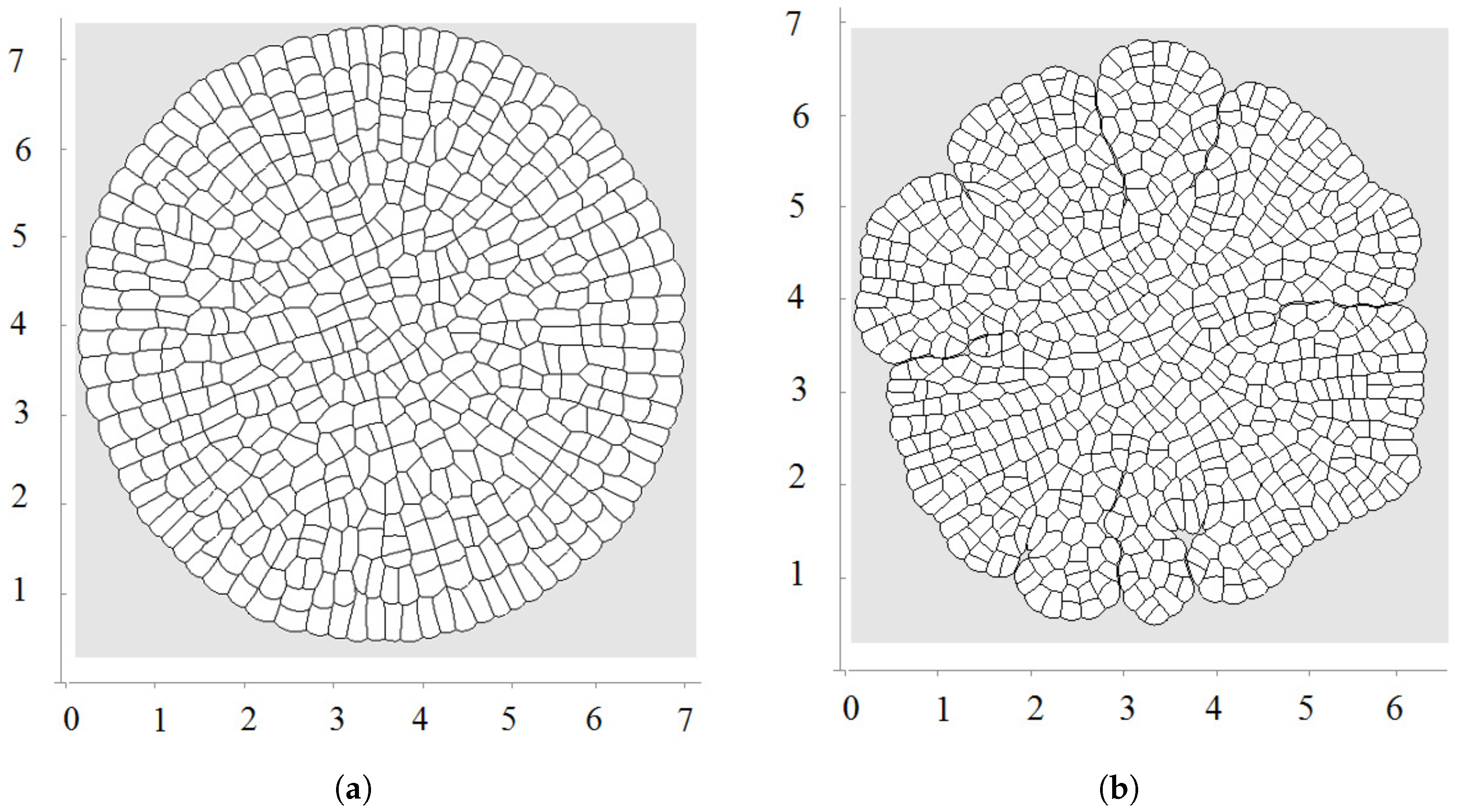
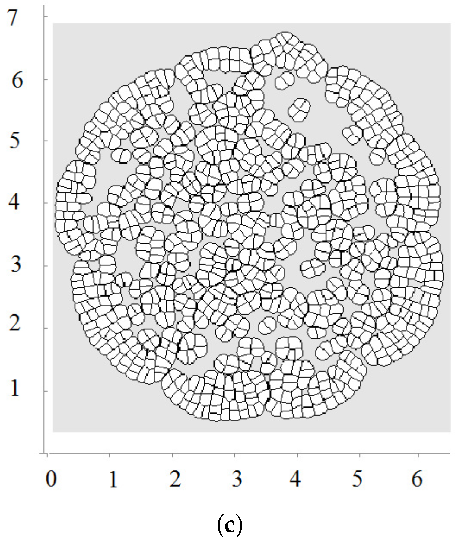
Figure 5.
Maximal pressure in the growing cell tissue. (a) maximal pressure as a function of time; (b) maximal pressure at time for different values of viscosity coefficient . Dimensionless time and pressure units are used.
Figure 5.
Maximal pressure in the growing cell tissue. (a) maximal pressure as a function of time; (b) maximal pressure at time for different values of viscosity coefficient . Dimensionless time and pressure units are used.
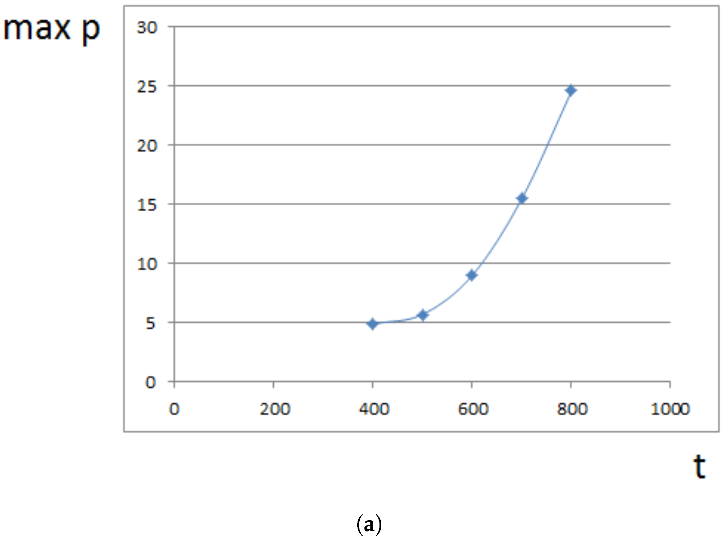
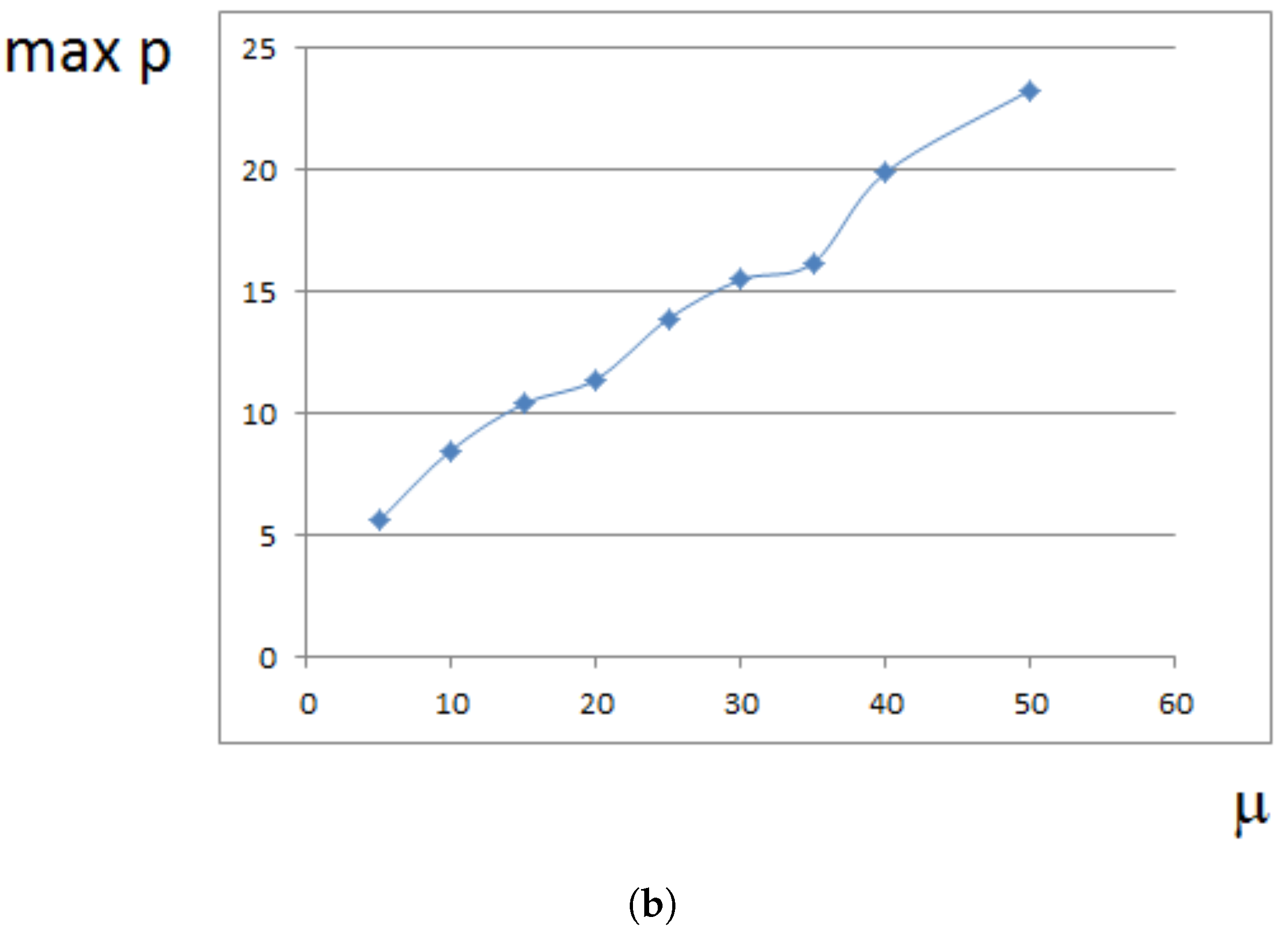
Figure 6.
A snapshot of growing tissue with an external supply of nutrients only to the outer cells (a) and with nutrient diffusing inside the tissue (b).
Figure 6.
A snapshot of growing tissue with an external supply of nutrients only to the outer cells (a) and with nutrient diffusing inside the tissue (b).
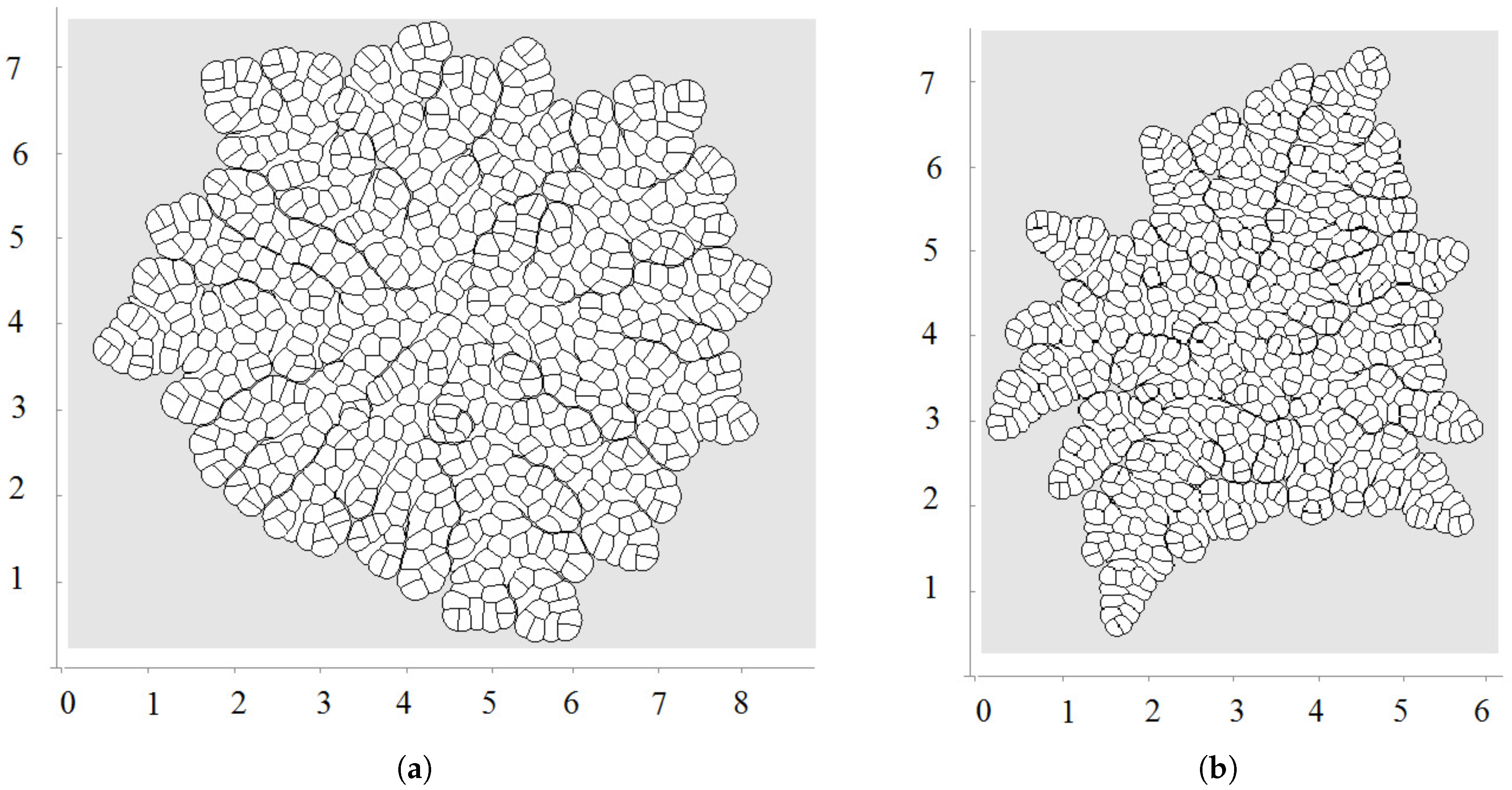
Figure 7.
Numerical simulations of wound healing. Original tissue (a); damaged tissue (b); tissue regeneration (c). Grey cells are fixed, while white cells divide and fill the missing part of the tissue.
Figure 7.
Numerical simulations of wound healing. Original tissue (a); damaged tissue (b); tissue regeneration (c). Grey cells are fixed, while white cells divide and fill the missing part of the tissue.

Figure 8.
Numerical simulations of wound healing. Original tissue (a); damaged tissue (b); tissue regeneration with equal rates of cell growth (c); cell growth rate depends on the initial position of the first dividing cell in its lineage (d).
Figure 8.
Numerical simulations of wound healing. Original tissue (a); damaged tissue (b); tissue regeneration with equal rates of cell growth (c); cell growth rate depends on the initial position of the first dividing cell in its lineage (d).

Figure 9.
Comparison of numerical simulations (continuous curves) with the analytical model (dots) for different values of parameters. (a) tissue growth with a constant proliferation rate in logarithmic coordinates. Linear dependence corresponds to the exponential growth. 1. , , ; (b) quadratic growth for pressure-dependent proliferation, 1. , 2. . Dimensionless time and area units are used.

© 2017 by the authors. Licensee MDPI, Basel, Switzerland. This article is an open access article distributed under the terms and conditions of the Creative Commons Attribution (CC BY) license (http://creativecommons.org/licenses/by/4.0/).
Share and Cite
MDPI and ACS Style
Bessonov, N.; Volpert, V. Deformable Cell Model of Tissue Growth. Computation 2017, 5, 45. https://doi.org/10.3390/computation5040045
AMA Style
Bessonov N, Volpert V. Deformable Cell Model of Tissue Growth. Computation. 2017; 5(4):45. https://doi.org/10.3390/computation5040045
Chicago/Turabian StyleBessonov, Nikolai, and Vitaly Volpert. 2017. "Deformable Cell Model of Tissue Growth" Computation 5, no. 4: 45. https://doi.org/10.3390/computation5040045
Note that from the first issue of 2016, this journal uses article numbers instead of page numbers. See further details here.