Trajectory Optimization of Electrostatic Spray Painting Robots on Curved Surface

1
School of Electronics and Information, Jiangsu University of Science and Technology, Zhenjiang 212003, China
2
School of Automation, Southeast University, Nanjing 210096, China
3
School of Science, Jiangsu University, Zhenjiang 212013, China
*
Author to whom correspondence should be addressed.
Coatings 2017, 7(10), 155; https://doi.org/10.3390/coatings7100155
Submission received: 16 August 2017
/
Revised: 21 September 2017
/
Accepted: 22 September 2017
/
Published: 25 September 2017
(This article belongs to the Special Issue Innovative Coatings for Automotive Industry)
Abstract
:In this paper, a new practical electrostatic rotating bell (ESRB) cumulative rate model of painting is derived, and an experimental study on painting is carried out. First, the experimental method is used to obtain the radial thickness profile function of the spatial paint distribution of static spray. Then, a spatial trajectory-planning scheme for a spray-painting robot based on a rectangular model is presented. This method designs the spatial path of the spray-painting robot by using the cuboid model method after the optimal value is taken as the width d of the overlapping area of the two spray-painting strokes in the plane. The experimental results illustrate that the paint thickness basically meets the requirements, and the experimental results verify the effectiveness of the trajectory optimization method.
1. Introduction
An electrostatic spray-painting robot is a very important piece of painting production equipment. It uses a high-voltage electrostatic field to improve the efficiency of paint deposition, and is globally used in the coating production lines of automobile. Trajectory optimization consists of two parts: path planning, and spray speed optimization. The trajectory of the electrostatic spray-painting robot has a great impact on the spraying quality of the objectives. Therefore, many scholars are researching on the trajectory optimization algorithm, control strategy, and off-line programming system of electrostatic spray-painting robots in recent years.
The high-voltage electrostatic spray-painting technology with a high-speed rotary bell used in spray-painting robots was developed by the BMW Company in Germany, which has greatly promoted the development of spray painting technology. Compared with air spraying, the electrostatic rotating bell atomizer (ESRB) is highly efficient, and the utilization rate of paint is three times higher than air spraying [1]. However, it can be influenced by many factors, such as the rotating speed, the distance between the rotary bell and the workpiece, the curvature of the workpiece, the air flow field, the electrostatic field, the trajectory of droplets, the quantity of electric charge, and others. The establishment of its model involves mathematics, control, electronics, fluid mechanics, and so on. In order to improve product quality and production efficiency, save paint, reduce environmental pollution, and so on, the electrostatic rotary bell is mainly used in modern automobile body painting. Electrostatic spray painting with a high-speed rotary bell makes the workpiece grounded as the anode, and the electrostatic rotary bell connected to the negative high-voltage (−50~−120 kV) as the cathode. Rotary bells are driven by air turbine. The no-load speed is up to 70,000 r/min, and the load speed is up to 20,000–70,000 r/min [2]. When the paint is sent to the rotary bell rotating at high-speed, due to the centrifugal effect of the rotary bell, the paint on the inner surface of the rotating cup stretches into a film and then gets great acceleration to move towards the edge of the rotary bell. Under the dual effect of centrifugal force and a strong electric field, the film is broken into tiny and charged droplets, which move towards the opposite polarized workpiece with the aid of the shaping air and the mode-control ring. The film is deposited on the workpiece surface, and then the coating is formed. When the caliber of the rotary bell is larger, the centrifugal force of the paint particles is larger, and the atomized paint becomes thinner. However, the gap of paint in the middle is also increased. The difference between the middle and both sides of the spray pattern is also increased, which results in poor coating uniformity. So, the hollow area of the spray pattern, which is important for the large area spraying, needs to be reduced.
Previous researchers have used simple planar deposition models to establish geometric projective models, such as the rotation model, which is based on the rotated parabolic thickness profile [3], the bivariate Gaussian model [4], the Cauchy or Gaussian distributions model [5], and the beta distribution model [6]. However, the paint deposition model of the electrostatic rotating bell atomizer is significantly different from the model presented earlier. Conner et al. [6,7,8] proposed a highly accurate double Gaussians paint deposition model based on an ESRB spray gun, by using an offset 1-D Gaussian revolved about the axis of the spray gun, and a 2-D Gaussian centered at the origin of the deposition model plane to capture the shape of the paint distribution. In this article, a new practical ESRB cumulative rate model of painting is derived, and the experimental study on painting is carried out after using the experimental method to obtain the radial thickness profile function of the spatial painting distribution of static spray.
2. ESRB Spray Painting Model
As ESRB is closely related to many parameters (electrostatic voltage, diameter of paint droplets, rotating speed of the rotary bell, concentration and flow of paint, surface geometry, spray distance and speed of the rotary bell, etc.), it is difficult to establish a more accurate ESRB mathematical model. The existing studies on the ESRB spray-painting model are carried out by the experimental method under ideal conditions on a two-dimensional plane, while research studies on spray-painting models used for curved surfaces need improvement [9,10,11,12]. A new practical ESRB cumulative rate model of painting is proposed.
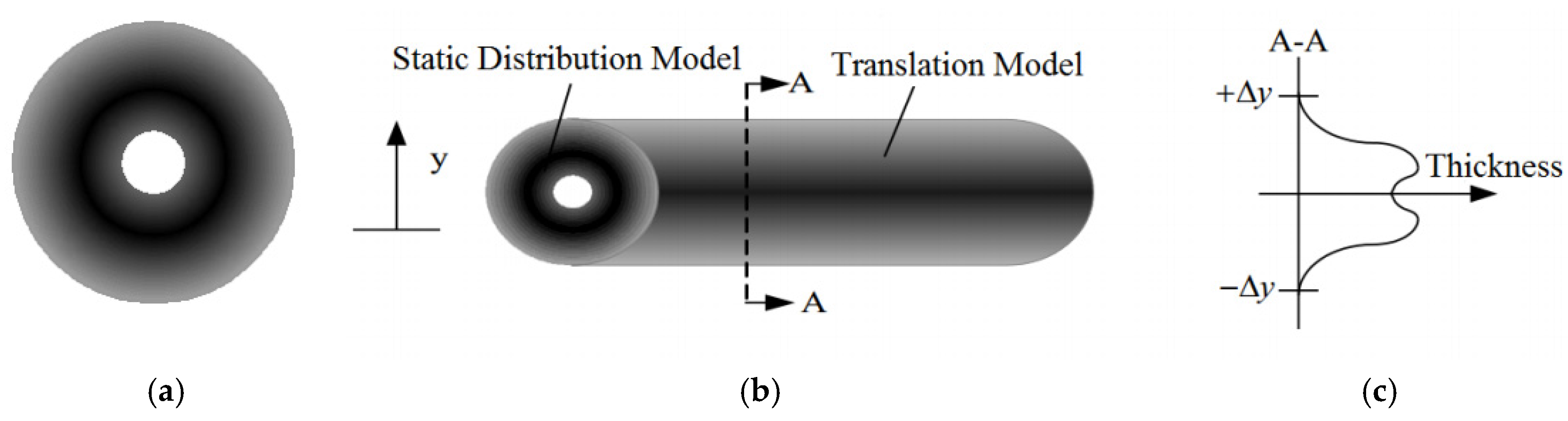
According to a large number of simulation experiments and spray painting experiments, we can see that the atomization of paint is caused by the centrifugal force generated by the high-speed rotation of the ESRB, the electric force of high-voltage static electricity, and the inertia force of shaping air. The spatial distribution of paint is a ring [13,14,15,16]. When the electrostatic voltage, spray painting distance, rotating speed of the rotary bell, paint flow, viscosity of paint, and other parameters keep certain, the ESRB is perpendicular to the workpiece surface and is sprayed at a fixed point for a period of time. The resulting paint space is then distributed as a hollow ring, as shown in Figure 1a.
As shown in Figure 1b, when the ESRB moves along the direction A, a stripe-shaped paint deposition area is formed. While moving, the coating thickness of the middle is small because of the hollow area in Figure 1a, and the coating thickness of both sides grows. Figure 1c shows the cross-sectional figure of the paint thickness along the A–A direction corresponding to the deposition of the striated paint in Figure 1b, which shows the variation function of the paint thickness in the y-direction.
Suppose that the radial thickness profile function of the spatial distribution of the static paint on the plane is h(r); then, the function image is shown in Figure 2. The static radial thickness profile in the figure represents an axisymmetric static spray profile. In order to convert this axisymmetric static spray profile into a dynamic profile or striped paint deposition area, this axisymmetric static spray profile needs to be converted to a circular spray painting model. As shown in Figure 2, the circular spray model can be obtained by rotating the thickness profile around the axis of symmetry.
As shown in Figure 3, assuming that the integral of the static spray profile along the spraying direction is H(y), the radial thickness profile h(r) of the circular static spray model can be accumulated to form a cross-sectional thickness profile H(y) along the spraying direction, and the function H(y) is the cumulative paint thickness in the y-direction.
Assuming that the translational velocity of the ESRB is v, if the rotary bell translates along the x-direction in Figure 3, the cumulative rate of the paint in the translation direction is the same in the plane, H(y) is the integral of the paint thickness on the string whose length is s(y). The expression is:
where . Since the radius r is a function of the distance x, Equation (1) can be transformed into:
Furthermore, in order to obtain the paint thickness value on the string, it is necessary to perform coordinate transformation:
Since the value of y on the string is constant, dy = 0. Substitute into Equation (3):
Substitute Equation (4) into Equation (2):
Since Equation (5) may have singular points at r = y (i.e., x = 0), it is not easy to solve. It can be processed by the partial integration method; then, Equation (5) can be transformed into:
As the paint thickness is measured at the discrete paint sampling point in practical work. Therefore, we can make small enough, and let be a constant between r and . By processing Equation (6) with the numerical integration method, we can get:
After further processing, we can get:
So far, as long as we obtain the radial thickness profile data of ESRB in unit time, we can obtain the paint deposition rate in the movement of ESRB, according to Equation (8).
3. Spatial Path Planning Based on Cuboid Model
Here, a cuboid model method is proposed to design the spatial path of the spray-painting robot. In this method, the key factor is determining the width d of the overlapping area of the two spray-painting strokes. Figure 4 shows a flow chart for calculating the optimized value of width d of the overlapping area formed by two spray painting strokes.
After finding the optimal value of the width d of the overlapping area of the two spray painting strokes on the plane, the following steps are taken to design the spatial path of the spray-painting robot by the cuboid model method:
- 1)
- The surface is determined by the CAD (Computer Aided Design) model of the workpiece, and the surface is divided into triangular meshes. After triangulating the surface, we can express it as a mathematical expression:where Ti is the i-th triangle in the triangular facet, and M is the total number of triangular facets in the triangular mesh.M = {Ti: i = 1, …, M}
- 2)
- Calculate the normal vector of each triangular facet, and generate a number of large patches according to the topology between adjacent triangular facets. Then, suppose that the normal vector of the surface and the normal vector of the projection plane of the surface both have the maximum angle βth (only consider that the normal vectors of the two are on the same side of the surface). After determining βth, each patch of the surface can be generated. The steps of connecting the respective triangular facets into patches are as follows:
- (1)
- Specify any of the triangular facets as the initial triangular facet.
- (2)
- Find all triangular facets that are less than the spray radius from the center point of the initial triangular facet.
- (3)
- Calculate the angle between the normal vector of all triangular facets found in Step (2) and the normal vector of the original triangular facet. If the angle is smaller than βth, connect the triangular facet with the initial triangular facet.
- (4)
- Look for the triangular facets that have not been connected into patches as a new initial triangular facet, and repeat Steps (2) and (3) until all of the triangular facets are connected into patches.
After patching the surface, any one of the patches can be expressed as:
In the expression above, Si denotes the j-th patch, and and are the normal vectors of the j-th triangular facet and the k-th triangular facet, respectively. D(Tj,Tk) denotes the distance between the i-th triangular facet and the center point of the k-th triangular facet. As a result, a surface will be divided into one or several patches. It is known to all that a quartic polynomial model can represent many 3D curved surfaces. After connecting the triangular facets into patches, each patch can be processed by the 3L algorithm, resulting in a smooth surface that retains the original properties [17,18,19,20].
- 3)
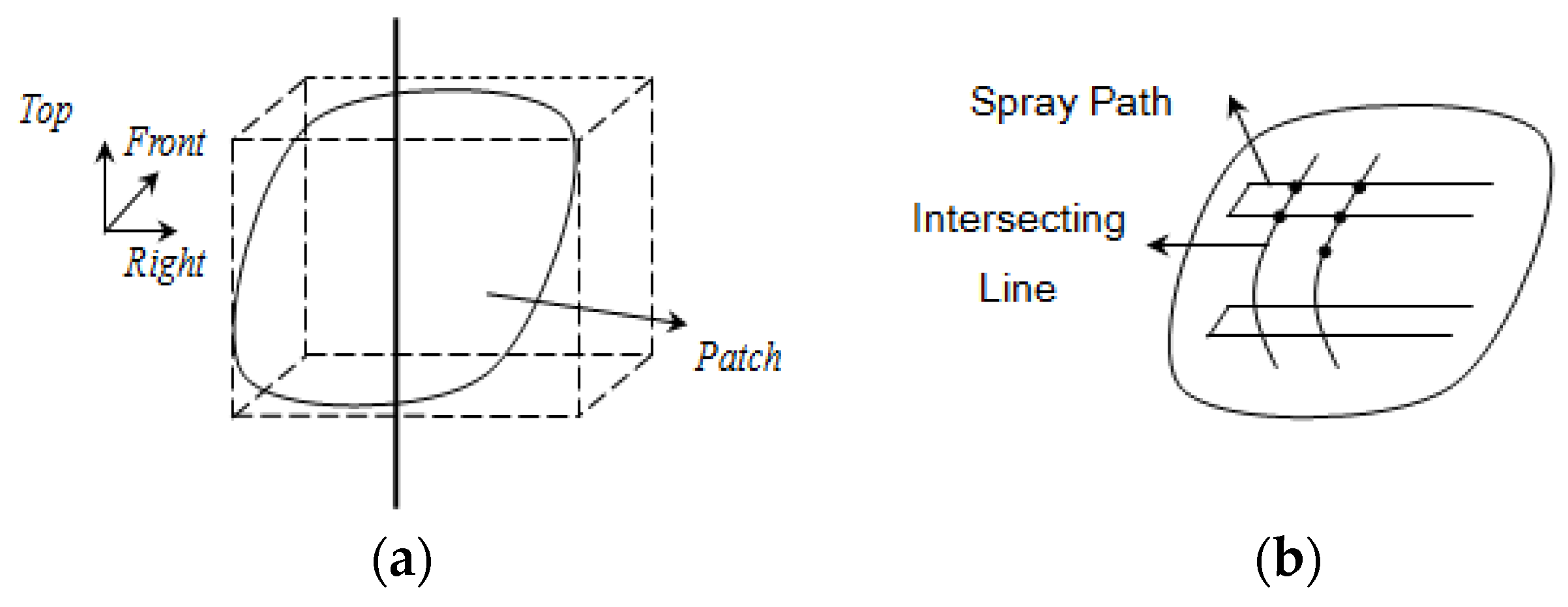
- The cuboid model is established on each patch, and the spatial path of the spray-painting robot on each patch is generated. Figure 5a shows the cuboid model established on a patch. The cuboid model is a cuboid that contains exactly the entire patch, which has two main properties: (i) its leading direction is opposite to the direction of the normal vector of the entire patch, and (ii) the area of the rectangle on each facet is as small as possible. In order to generate the spatial path of the spray-painting robot, firstly, a number of tangent planes whose distance are l (l is taken as R/2–R, R is the spray radius) are taken along the direction perpendicular to the right side of the cuboid model. Then, the intersection between the tangent plane and several segments of the curved surface can be obtained, and a series of points whose distance is d (the optimum value of the overlapping area’s width formed by two spray-painting strokes) are uniformly made on the intersecting line. Finally, these points are connected along the right side of the cuboid mode to generate the spatial path of the spray-painting robot (as shown in Figure 5b).
4. Electrostatic Spray-Painting Experiment
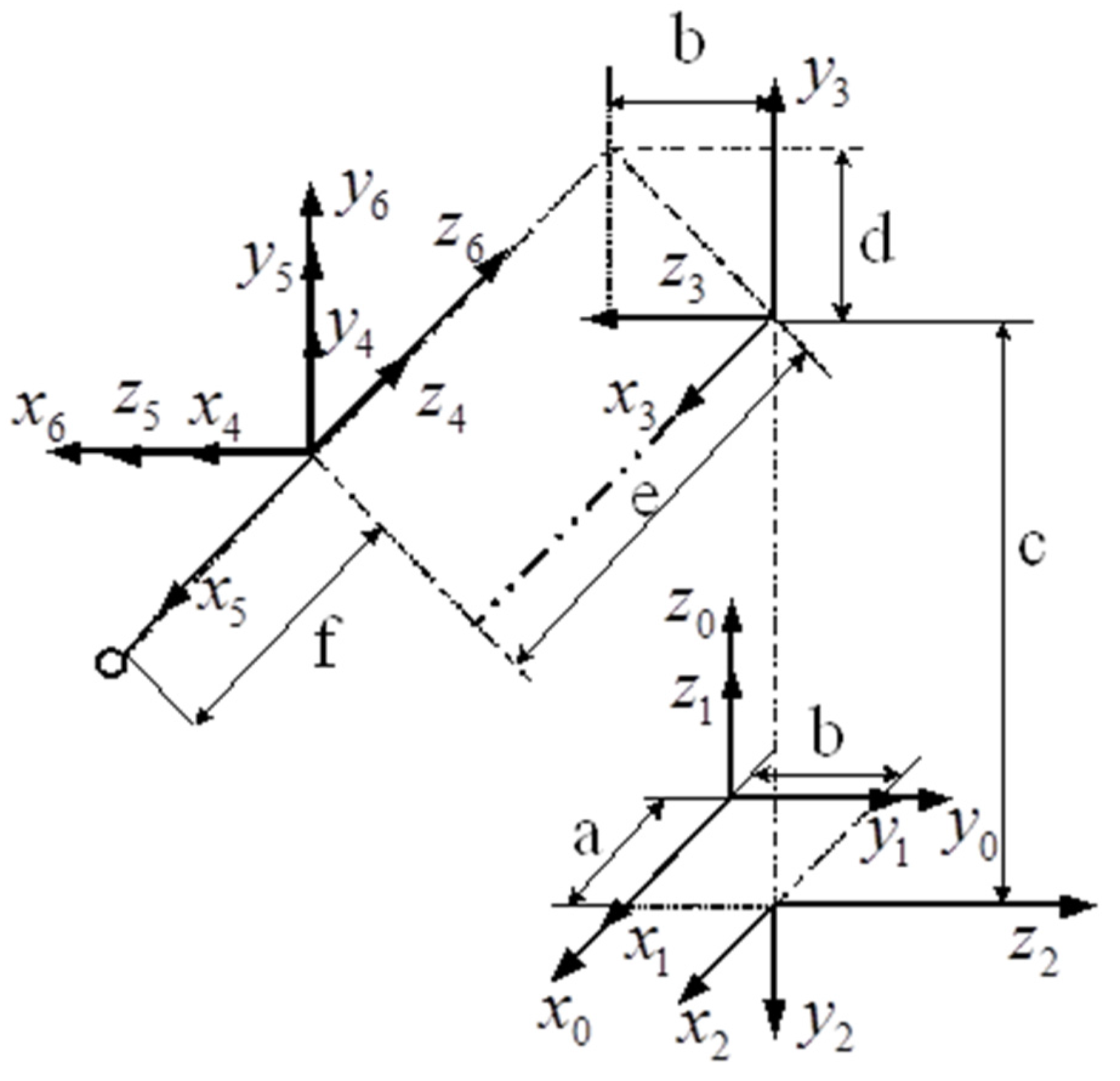
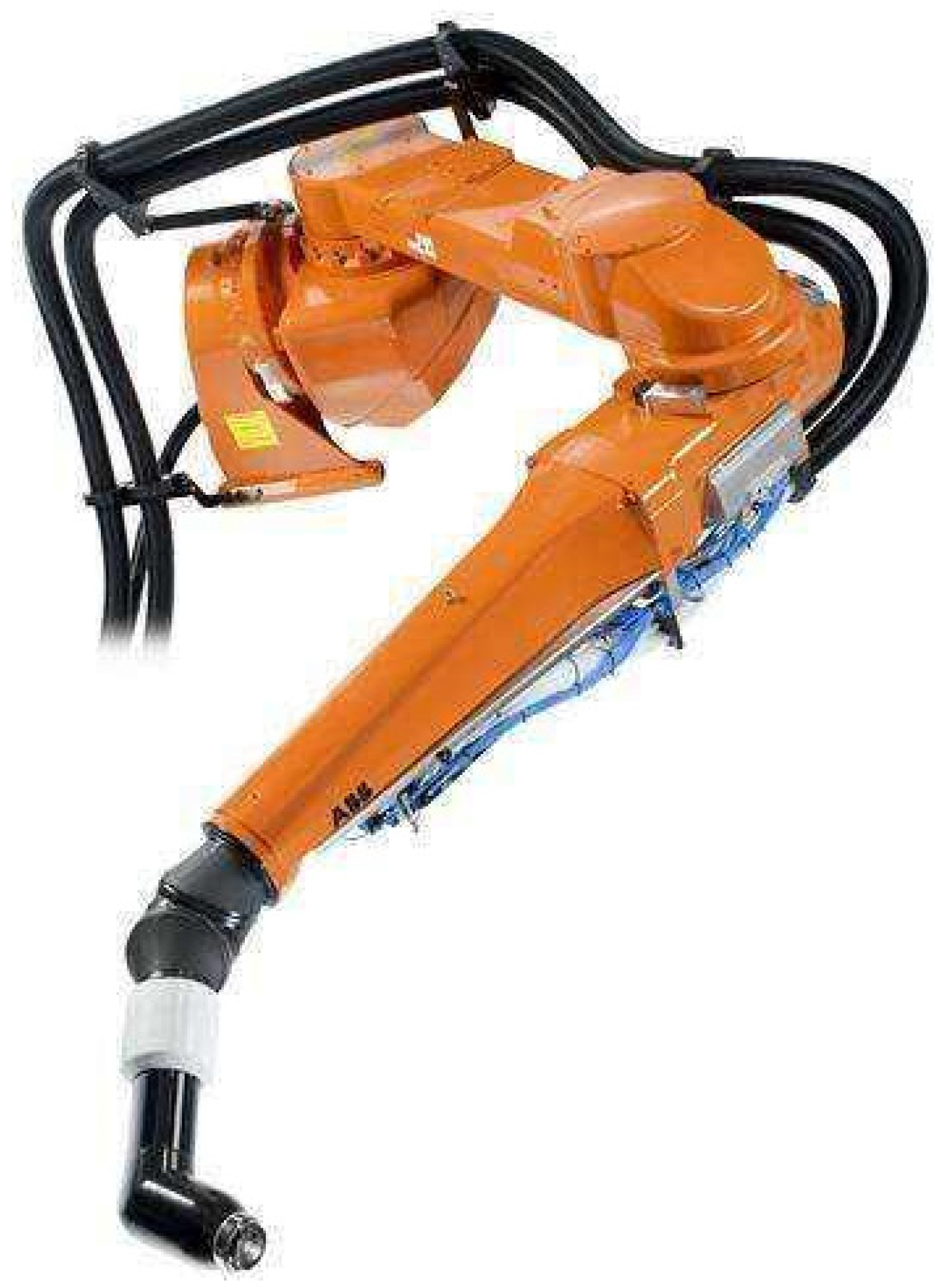
Taking the automotive body of a certain brand as the paint objective, we use the ABB electrostatic spray-painting robot (Asea Brown Boveri Ltd., Zurich, Switzerland) to perform the varnish spray experiment. The joint coordinates and parameters of the painting robot are shown in Figure 6. The robot uses the ESRB spray mode, as shown in Figure 7. This is a double-shaping air system with straight nozzles, and the bell diameter is 60 mm. The body is divided into four portions: a roof portion, a left portion of the car, a right portion of the car, and a rear portion. Since the left and right sides are completely symmetrical, only one side is listed. These portions can be sprayed in several zones by four spray-painting robots, as shown in Figure 8.
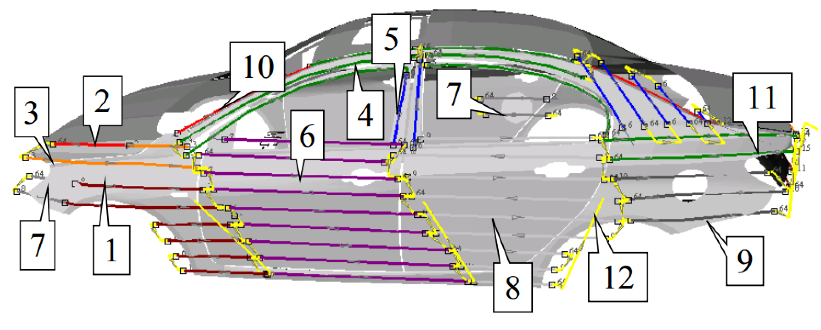
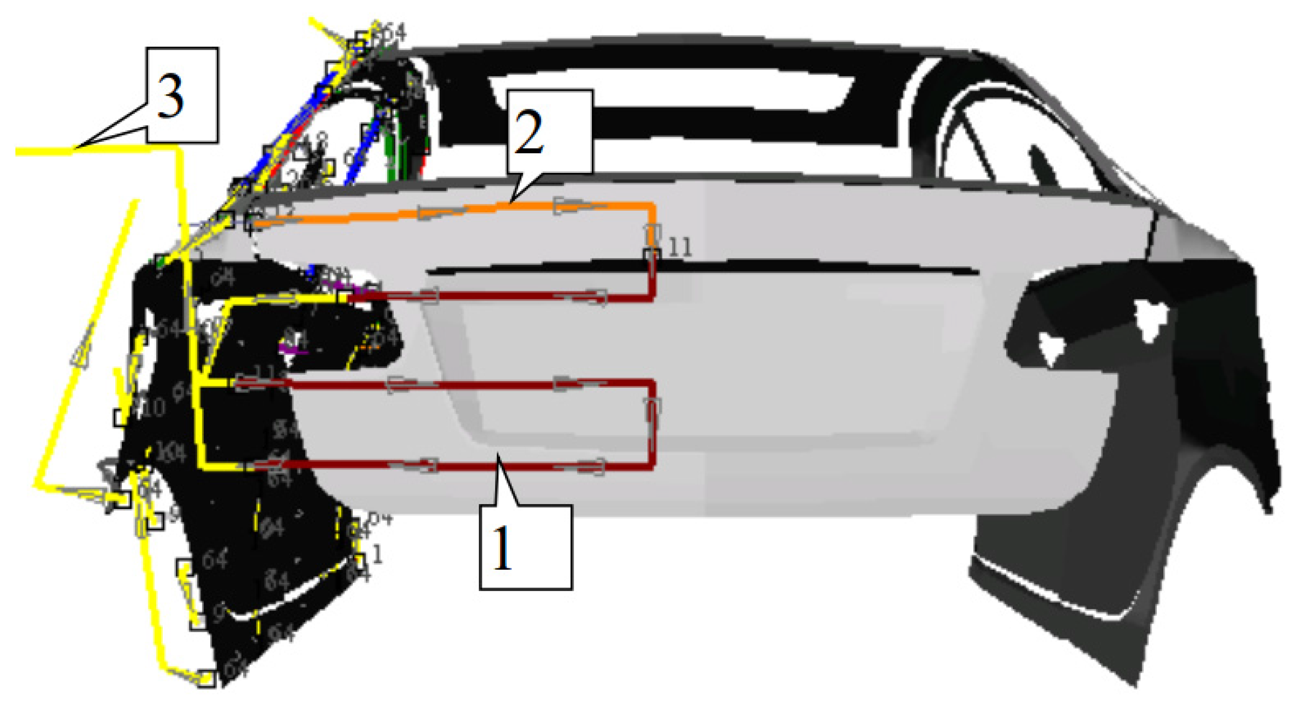
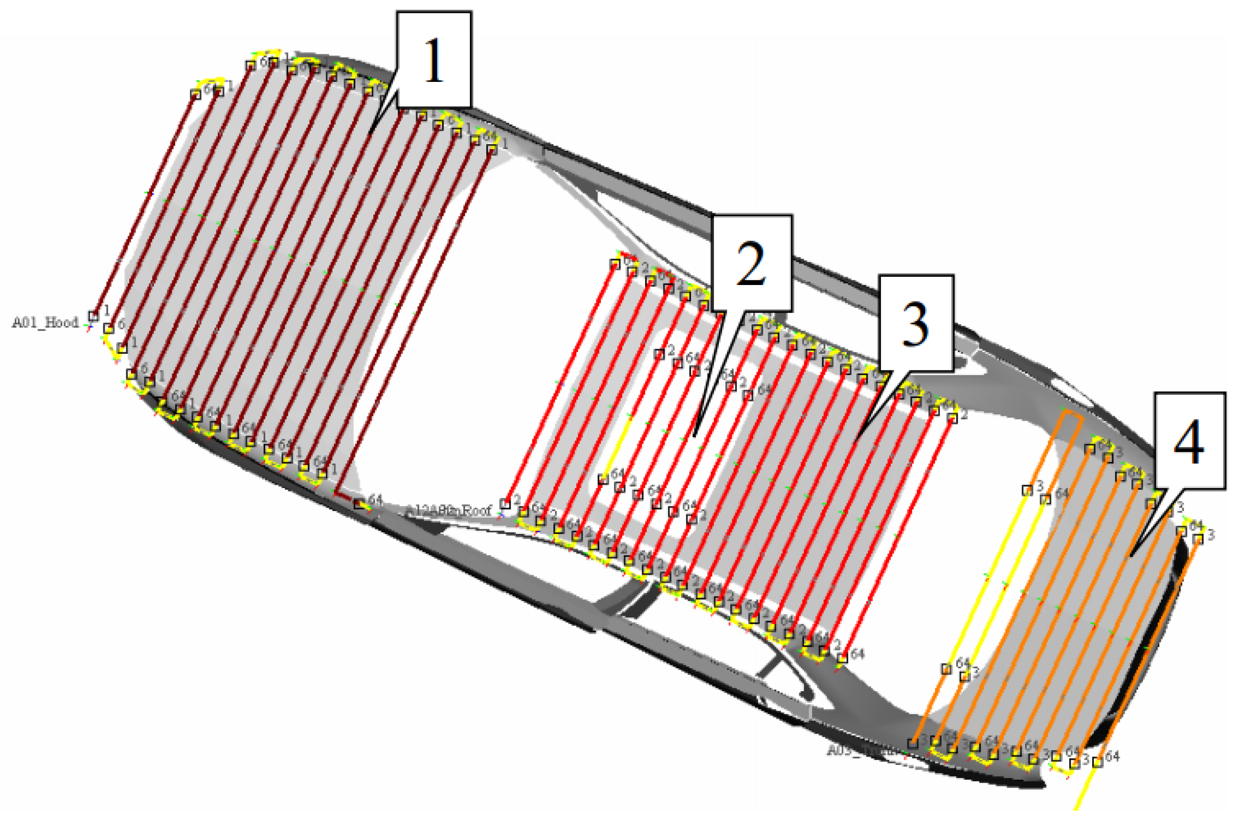
According to the spray model of ESRB and the trajectory optimization method of the spray-painting robot, the trajectory planning is carried out on the four portions of the automobile body. According to the different curvature of the surface and the different shape of the workpiece, we use different trajectory distance, paint flow, and shaping air flow parameters in the planning process. According to the features of the experimental platform for the automobile spray-painting of the spray-painting robot, the joint motion of the robot is smaller and more stable, and the performance is better when the end effector ESRB of the robot moves at uniform speed. Compared with other types of end effectors, the use of the optimal paint flow control can completely replace the optimization method for spray-painting speed in the course of the experiment, as the ESRB itself has an excellent paint flow real-time control adjustment function. That is, after the trajectory optimization for the spray-painting robot is performed in the off-line programming system, the corresponding large paint flow rate is used to paint at the place on the trajectory where the robot needs to move slowly. Conversely, the corresponding small paint flow rate is used to paint at the place on the trajectory where the robot needs to move quickly. Of course, a functional relationship between the moving speed of the spray-painting robot and the paint flow rate needs to be established in this process. This relationship is obtained through the large amount of data after the experimental calibration of the spray-painting robot. The optimized spray trajectories generated by the roof portion, the left portion of the car, and the rear section are shown in Figure 9, Figure 10 and Figure 11, respectively. The roof portion of the car is divided into seven segments of optimization trajectory (the location number of each trajectory has been marked in the figure), the left portion of the car is divided into 12 segments, and the rear portion is divided into three segments. The different segments of the optimization trajectory in the off-line programming system of the spray-painting robot are indicated with different colors. The spray-painting parameters corresponding to each portion of the optimization trajectories are shown in Table 1, Table 2 and Table 3, respectively.
In Table 1, Table 2 and Table 3, the parameter Del represents the paint flow rate, AM represents the rotating speed of the rotary bell, SA1 represents the flow of air 1, SA2 represents the flow of air 2, and HV represents the electrostatic voltage of the rotary bell. Air 1 is used to drive the turbine and rotate the rotary bell; air 2 is shaping air. Among the tables above, the paint flow of the yellow trajectory is zero (i.e., the No. 7 trajectory in Table 1, the No. 12 trajectory in Table 2, and the No. 3 trajectory in Table 3); the ESRB does not spray, and the spray-painting robot transfers its position at this time.
When the trajectory on the surface of the automobile is all planned, the information is input into the controller of the spray-painting robot. Now, the spray-painting trajectory is “the spray painting path based on the workpiece being sprayed”, and is not the trajectory of the spray-painting robot. The spray-painting robot will transform the spray path based on the workpiece into the spray path of the actual spray-painting robot according to the conveyor speed of the conveyor belt, the CAD model of the automobile body, the spatial position, and other information of the calibrated individual robots and the automobile body. In other words, it is the trajectory of each joint of the spray-painting robot. In this process, it is necessary to transform between the spatial coordinate system of the workpiece and the base coordinate system of the robot (also called workpiece calibration). The transformission between the coordinate system of the end effector and the base coordinate system of the robot is also necessary (also called tool calibration) [21,22,23,24].
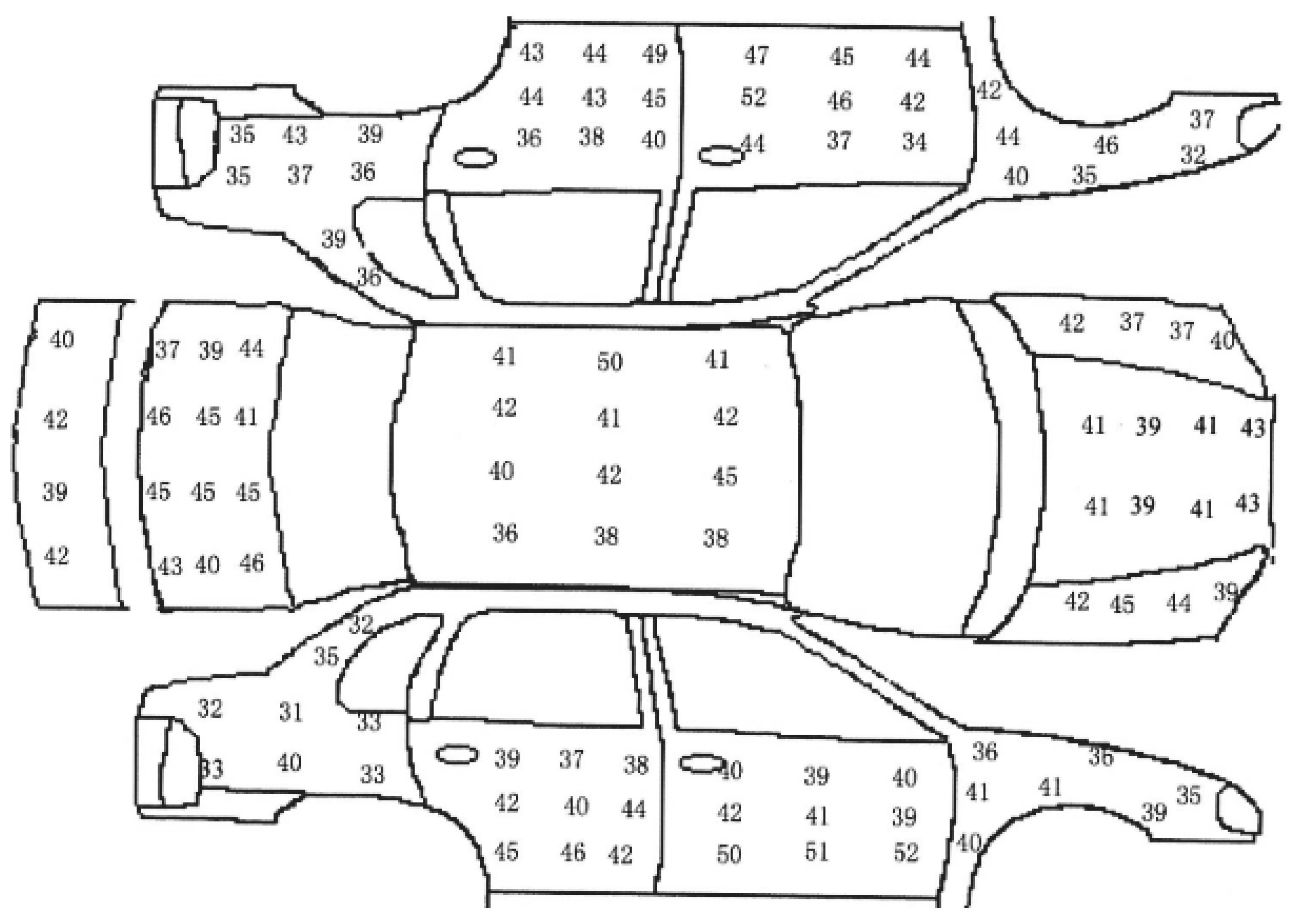
After the paint operation is finished, we dry the paint on the automobile body, and then use the professional QuaNix®7500 (QNIX, Cologne, Germany) coating thickness gauge to measure the coating thickness at each sampling point on the surface of the tested automobile body surface. The coating thickness data at each sampling point is shown in Figure 12. The position of the data in the figure is the corresponding position on the automobile body when the automobile is detected, so we can see the uniformity of coating thickness at all parts of the automobile body clearly. At this point, the reason for the difference in the uniformity of coating thickness can be analyzed according to the surface shape of the corresponding position on the automobile body.
According to the actual spray-painting requirements in the production process of the brand car, the ideal coating thickness is qd = 40 × 10−6 m, and the deviation of the maximum coating thickness is qw = ±5 × 10⁻⁶ m. The coating thickness curve of each sampling point on the automobile body is shown in Figure 13. The thin curve in the figure is the variation curve of the coating thickness, and the data entry has the basic distribution according to the position in Figure 12: First is the left portion of the car, from the rear to the front. Second is the automobile body, from the front to the rear. Last is the right portion of the car, from the front to the rear. The thick solid line in the figure is the upper and lower limits of the standard thickness. It can be seen from the graph that only the coating thickness of some discrete points exceeds the upper and lower limits of the coating thickness. The coating thickness basically meets the requirements, and the experimental results verify the effectiveness of the trajectory optimization method.
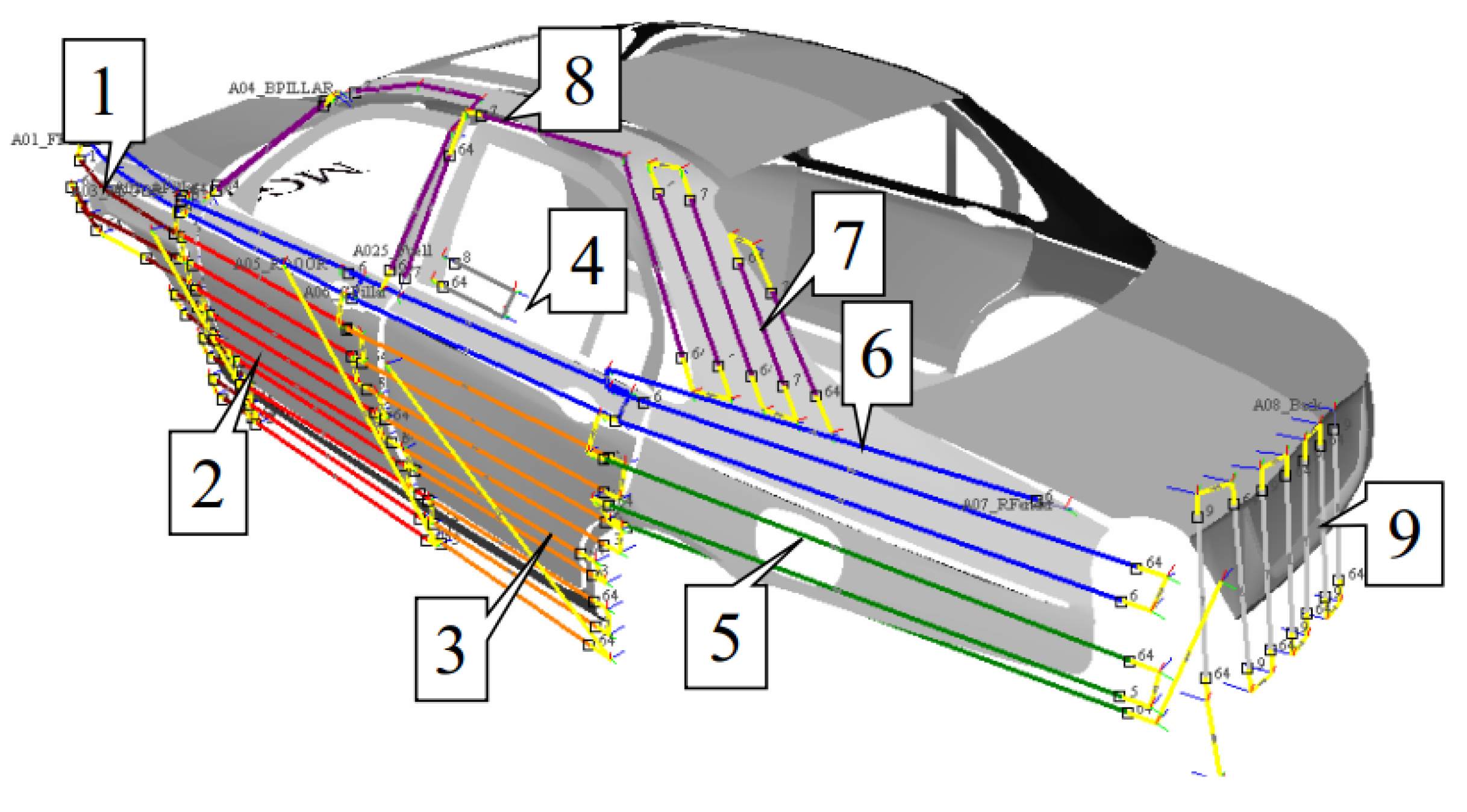
Another varnish spray experiment on the same automotive body is performed. The trajectory planning is carried out on the surface of the same automotive body along the v-direction. The body is divided into three portions: the roof portion, the left and left-rear parts of the car, and the right and right-rear parts of the car. The optimized spray trajectories generated by the roof portion, the left and left-rear parts, and the right and right-rear parts are shown in Figure 14, Figure 15 and Figure 16, respectively.
The roof portion of the car is divided into four segments of optimization trajectory, the left side and rear left parts of the rear part are divided into nine segments, and the right side and right-rear parts are also divided into nine segments. The spray-painting parameters corresponding to each portion of the optimization trajectories are shown in Table 4, Table 5 and Table 6, respectively.
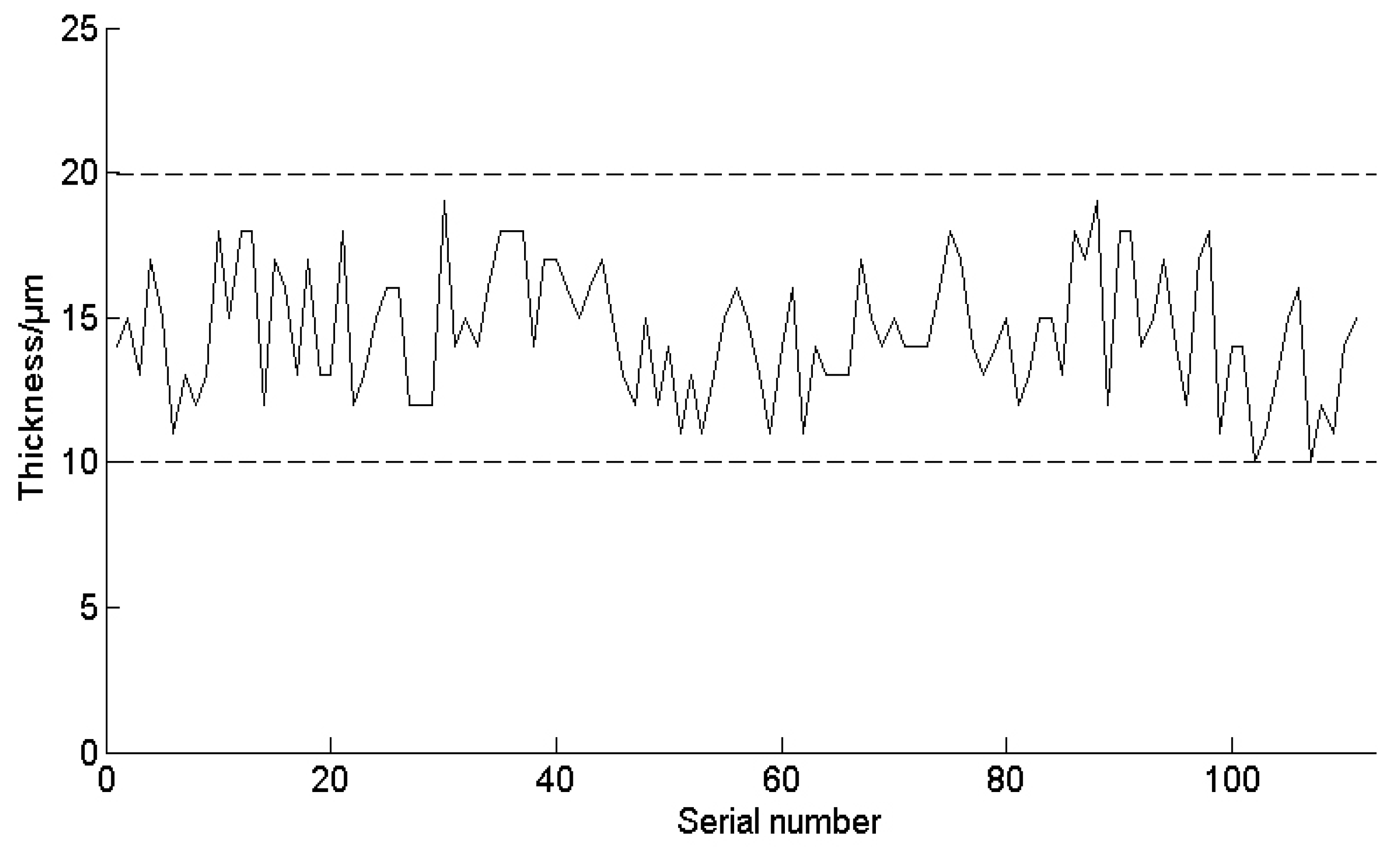
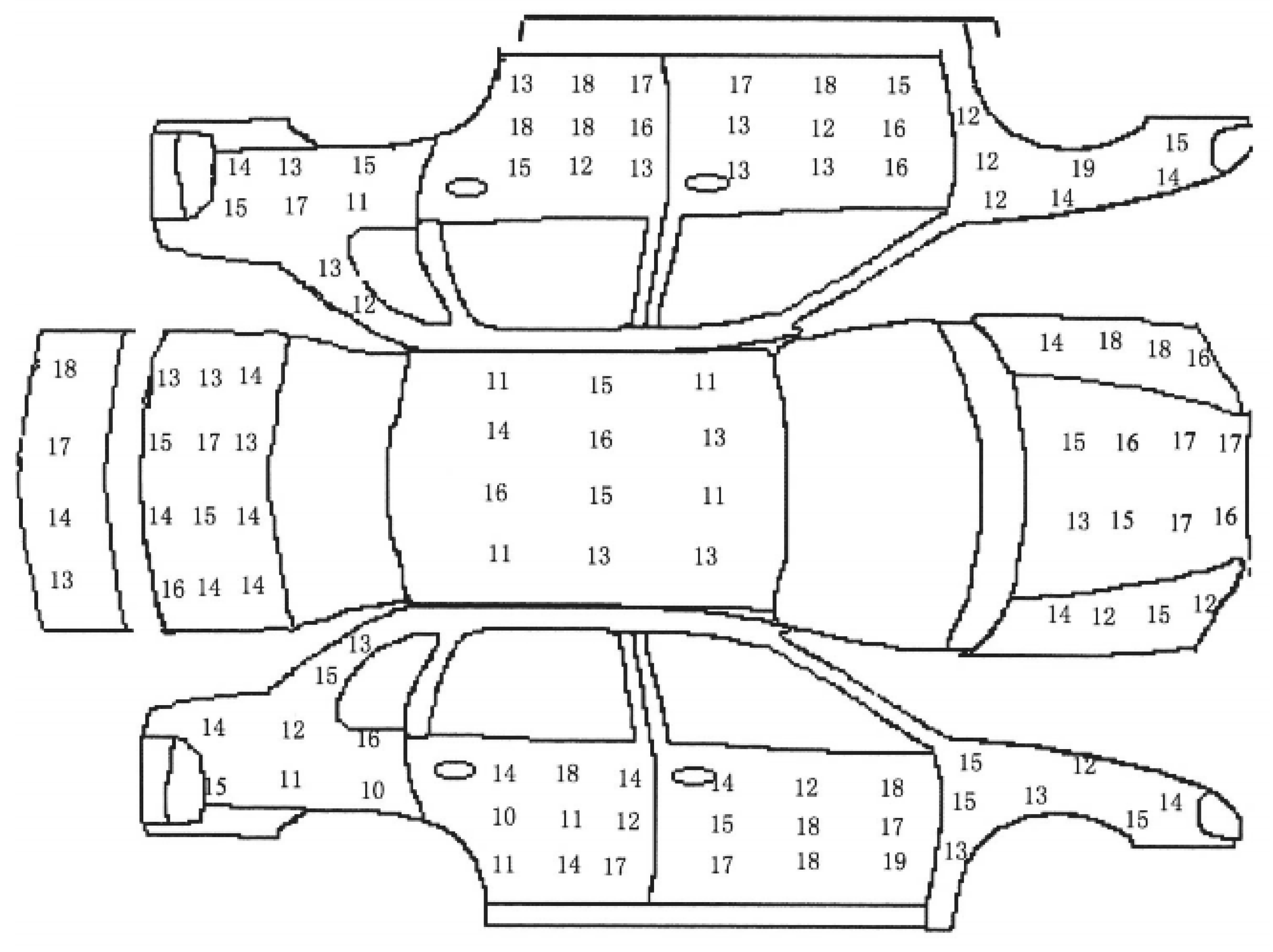
In order to distinguish from the first experiment, the ideal coating thickness is qd = 15 × 10−6 m, and the deviation of the maximum coating thickness is qw = 5 × 10⁻⁶ m. The paint thickness date at each sampling point is shown in Figure 17. The coating thickness curve of each sampling point on the automobile body is shown in Figure 18. The thin curve in the figure is the variation curve of the coating thickness, and the data entry has the basic distribution according to the position in Figure 17: The first part is the left side of the body, and the order is from the rear to the front. Then, the order of the second part is: the front, the roof, the rear. The last part is the right side, with the order from the front to the rear. The dotted line in Figure 18 is the upper and lower limits of the standard thickness. The coating thickness basically meets the requirements, and the experimental results verify the effectiveness of the trajectory optimization method.
According to the results of the two spraying experiments, the analysis of the reasons why the coating thickness in the partial area is beyond the upper and lower limits are as follows:
- The indicator requirements in the production process of spray-painting operation are rather high. The deviation of the maximum coating thickness set in the experiments is merely qw = ±5 × 10⁻⁶ m. For the general requirements of the spray-painting operation, the deviation of the maximum coating thickness is usually set as qw = ±10 × 10−6 m. According to this deviation threshold, the experimental result data can all meet the requirements.
- The performance of the existing spray equipment limits the consistency of the coating thickness. Due to the limitation of the memory capacity in the robot, the trajectory parameters cannot be changed unrestrictedly and continuously. Only a few trajectories can be used to approach the optimized trajectory, and the precision is not very high. When the curvature of the surface is large, the parameters of the optimized spray trajectory are greatly changed, but the parameters in the actual spray-painting operations do not change accordingly, which leads to the deviation between the results of trajectory optimization and those of the experiment.
- The curved surface of the tested automobile is too complicated. As the curved surface area of the tested automobile is large and complex and disposable spray painting is used for the whole automobile, the ESRB is in different directions when painting different parts of the body, and the effect of the gravity that affects the trajectory of the mist particles is not the same. Some parts of the surface are horizontal, some parts of the surface are tilted, and other parts of the surface are vertical. When the coating is sprayed to different surfaces, its attachment effect is also different under the influence of gravity, which is the main reason the paint thickness of the rear is small.
- Efficiency requirements of the spray painting operation are high. According to the optimization method of the spray path proposed in this paper, if we want to meet the higher spray painting requirements, more spray painting time will certainly be consumed, which will sacrifice the spray-painting efficiency. Therefore, in the actual spray painting process, the spray-painting effect and spray efficiency must reach a compromise.
5. Conclusions
Electrostatic spray-painting robots are of vital importance to reduce the hollow area of the painting pattern for large-area spray painting. A new practical ESRB cumulative rate model of painting has been developed, and a spatial trajectory planning scheme for the spray-painting robot based on the rectangular model is presented. Taking the automotive body of a brand as the paint objective, we use the ABB electrostatic spray-painting robot to perform the varnish spray-painting experiment. The experimental results illustrate that the paint thickness basically meets the requirements, and the experimental results verify the effectiveness of the trajectory optimization method.
Acknowledgments
This research is supported by the National Natural Science Foundation of China (No. 61503162, 51505193), Project funded by China Postdoctoral Science Foundation (2016M601691), Natural Science Foundation of Jiangsu Province in China (No. BK20150473) and Major Research and Development Project (Modern Agriculture) of Zhenjiang City (NY2015025).
Author Contributions
Wei Chen and Yang Tang conceived and designed the experiments; Wei Chen performed the experiments; Hao Liu and Junjie Liu analyzed the data; Hao Liu contributed reagents/materials/analysis tools; Wei Chen wrote the paper.
Conflicts of Interest
The authors declare no conflict of interest.
References
- Akafuah, N.; Poozesh, S.; Salaimeh, A. Evolution of the automotive body coating process—A review. Coatings 2016, 6, 24. [Google Scholar] [CrossRef]
- Akafuah, N.K.; Salazar, A.J.; Saito, K. Infrared thermography-based visualization of droplet transport in liquid sprays. Infrared Phys. Technol. 2010, 53, 218–226. [Google Scholar] [CrossRef]
- Sheng, W.H.; Xi, N.; Song, M. Automated CAD-guided robot path planning for spray painting of compound surfaces. In Proceedings of the IEEE International Conference on Intelligent Robots and Systems, Takamatsu, Japan, 30 October–5 November 2000; pp. 1918–1923. [Google Scholar]
- Freund, E.; Rokossa, D.; Roβmann, J. Process-oriented approach to an efficient off line programming of industrial robots. In Proceedings of the 24th Annual Conference of the IEEE Industrial Electronics Society, Aachen, Germany, 31 August–4 September 1998; pp. 208–213. [Google Scholar]
- Ramabhadran, R.; Antonio, J.K. Fast solution techniques for a class of optimal trajectory planning problems with applications to automated spray coating. In Proceedings of the IEEE Tansactions on Robotics and Automation, Aachen, Germany, 31 August–4 September 1998; pp. 519–530. [Google Scholar]
- Arikan, S.; Balkan, T. Process modeling, simulation and paint thickness measurement for robotic spray painting. J. Field Robot. 2000, 17, 479–494. [Google Scholar]
- Atkar, P.N.; Conner, D.C.; Greenfield, A. Hierarchical segmentation of piecewise pseudoextruded surfaces for uniform coverage. IEEE Trans. Autom. Sci. Eng. 2009, 6, 107–120. [Google Scholar] [CrossRef]
- Atkar, P.N.; Greenfield, A.; Conner, D.C. Uniform coverage of automotive surface patches. Int. J. Robotics Res. 2005, 24, 883–898. [Google Scholar] [CrossRef]
- Conner, D.C. Paint deposition modeling for trajectory planning on automotive surfaces. IEEE Trans. Autom. Sci. Eng. 2005, 2, 381–392. [Google Scholar] [CrossRef]
- Yuan, Z. Trajectory planning of Bezier curve based on improved genetic algorithm. J. Shanghai Dian Ji Univ. 2012, 15, 237–240. [Google Scholar]
- Jie, Z.; Zongyan, C.; Tiger, L.; Qingtao, L. Bézier curves of autonomous mobile robot path planning based on. J. Lanzhou Univ. 2013, 49, 249–254. [Google Scholar]
- Juhász, M.; Róth, Á. A class of generalized B-spline curves. Comput. Aided Geom. Des. 2013, 30, 85–115. [Google Scholar] [CrossRef]
- Soma, T.; Katayama, T.; Tanimoto, J. Liquid film flow on a high speed rotary bell-cup atomizer. Int. J. Multiph. Flow 2015, 70, 96–103. [Google Scholar] [CrossRef]
- Toljic, N.; Adamiak, K.; Castle, G.S.P. Three-dimensional numerical studies on the effect of the particle charge to mass ratio distribution in the electrostatic coating process. J. Electrost. 2014, 69, 189–194. [Google Scholar] [CrossRef]
- Kolakowska, E.; Smith, S.F.; Kristiansen, M. Constraint optimization model of a scheduling problem for a robotic arm in automatic systems. Robot. Autonom. Syst. 2014, 62, 267–280. [Google Scholar] [CrossRef]
- Gasparetto, A. Automatic path and trajectory planning for robotic spray painting. In Proceedings of the 7th German Conference on Robotics, Munich, German, 21–22 May 2012; pp. 211–216. [Google Scholar]
- Chen, H.P.; Sheng, W.H. Transformative industrial robot programming in surface manufacturing. In Proceedings of the IEEE International Conference on Robots and Automation, Shanghai, China, 9–13 May 2011; pp. 6059–6064. [Google Scholar]
- Chen, H.P.; Xi, N. Automated robot trajectory connection for spray forming process. J. Manuf. Sci. Eng. 2012, 134, 171–179. [Google Scholar] [CrossRef]
- Zeng, Y.; Gong, J.; Xu, N. Tool trajectory optimization of spray painting robot formany-times spray painting. Int. J. Control Autom. 2014, 7, 193–208. [Google Scholar] [CrossRef]
- Wei, C.; Yang, T.; Qiang, Z. A novel trajectory planning scheme for spray painting robot. In Proceedings of the 28th Chinese Control and Decision Conference, Yinchuan, China, 28–30 May 2016; pp. 7008–7012. [Google Scholar]
- Chen, W.; .Zhao, D. Path planning for spray painting robot of workpiece surfaces. Mathemat. Probl. Eng. 2013, 2013, 659457. [Google Scholar] [CrossRef]
- Tang, Y.; Yang, W.G.; Chen, W. Trajectory planning for spray painting robot of free-form surfaces. Appl. Mech. Mat. 2016, 543, 1309–1312. [Google Scholar] [CrossRef]
- Tang, Y.; Chen, W. Tool trajectory planning ofpainting robot and its experimental. In Proceedings of the IEEE International Conference on Mechatronics and Control, Jinzhou, China, 3–5 July 2014; pp. 872–875. [Google Scholar]
- From, P.J.; Gunnar, J.; Gravdahl, J.T. Optimal paint gun orientation in spray paint applications—Experimental results. IEEE Trans. Autom. Sci. Eng. 2013, 8, 438–442. [Google Scholar] [CrossRef]
Figure 1.
(a) Coating distribution of electrostatic rotating bell (ESRB); (b) Translation of the static distribution model; (c) the section thickness of the translation model.
Figure 1.
(a) Coating distribution of electrostatic rotating bell (ESRB); (b) Translation of the static distribution model; (c) the section thickness of the translation model.

Figure 2.
Spatial distribution of the circular coating formed by the rotational radial thickness profile.
Figure 2.
Spatial distribution of the circular coating formed by the rotational radial thickness profile.
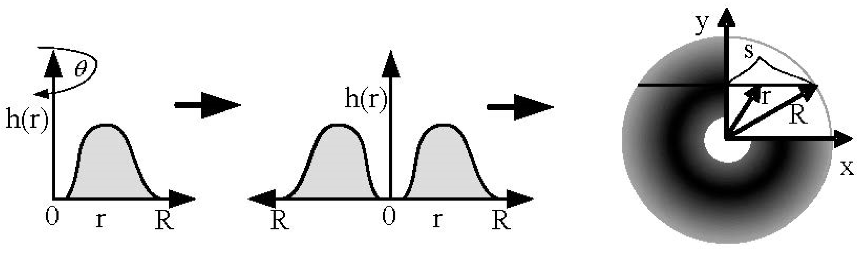
Figure 3.
Thickness profile of the circular deposition model, formed by the translational circular deposition model.
Figure 3.
Thickness profile of the circular deposition model, formed by the translational circular deposition model.
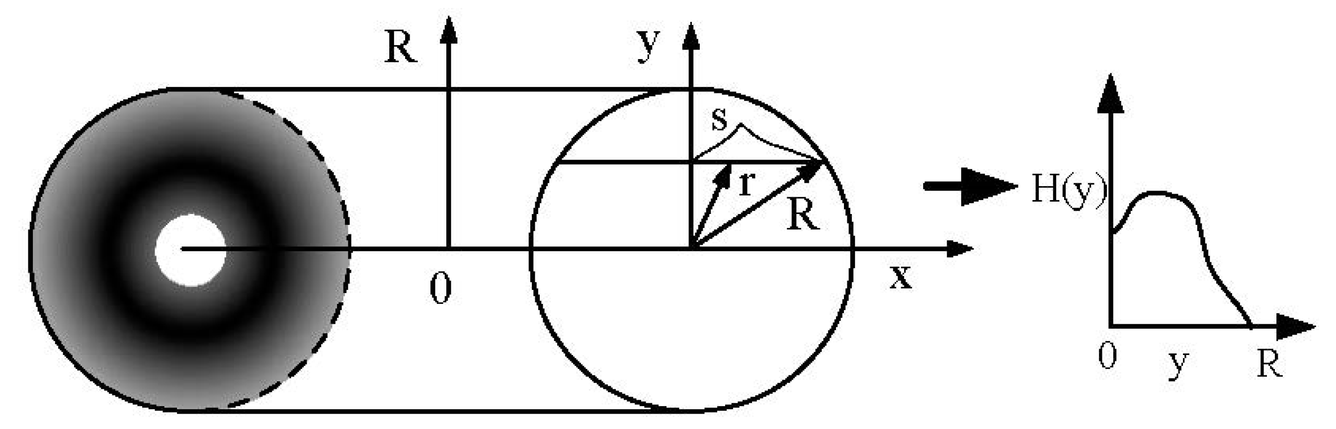
Figure 4.
Flow chart of the optimization of the width d of the overlapping area formed by two spray-painting strokes.
Figure 4.
Flow chart of the optimization of the width d of the overlapping area formed by two spray-painting strokes.
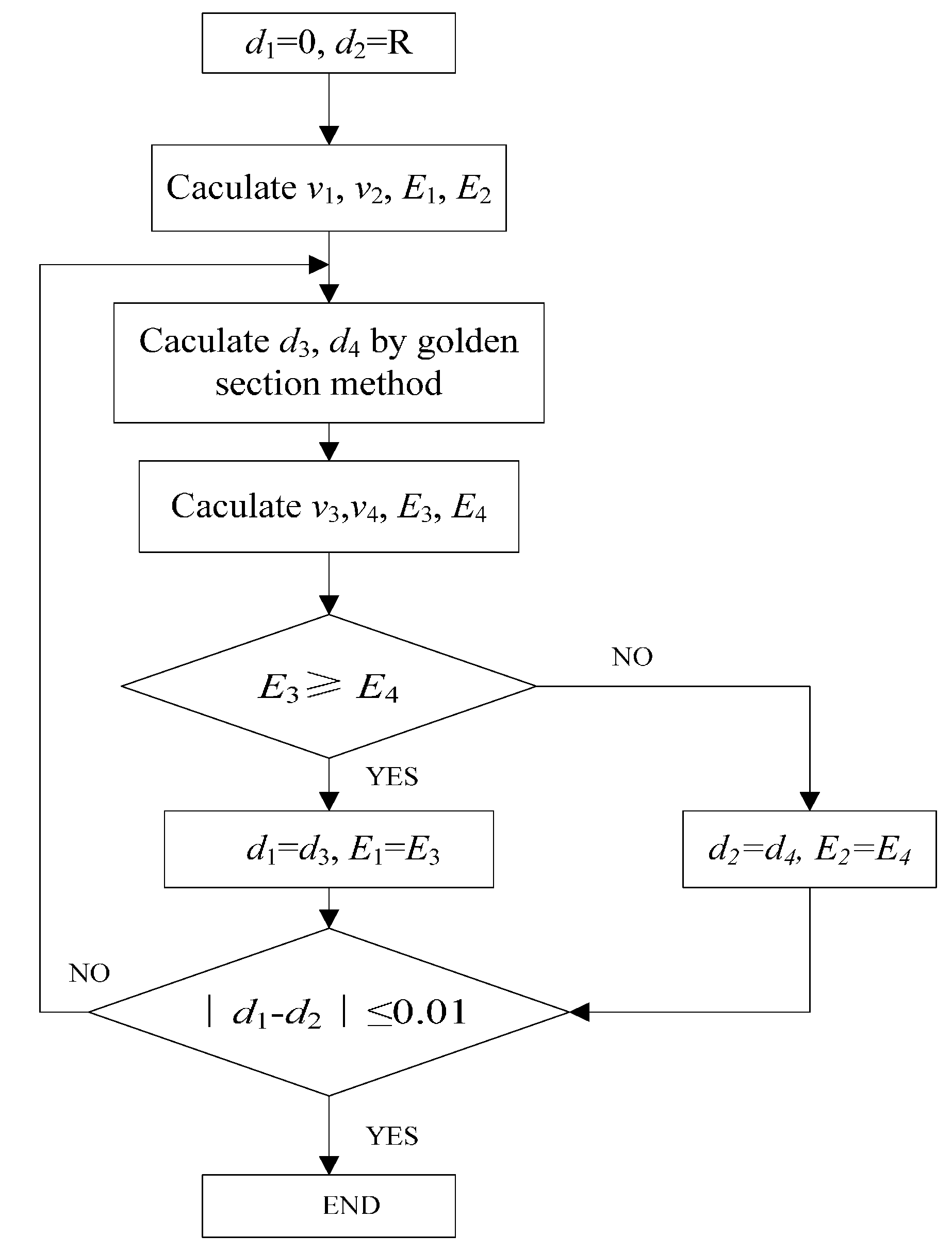
Figure 5.
(a) The cuboid model; (b) The generated spatial path.

Figure 6.
Joint coordinates and parameters of the ABB painting robot.

Figure 7.
ABB Spray-painting robot in a Company.

Figure 8.
An automobile paint line composed by several spray-painting robots.
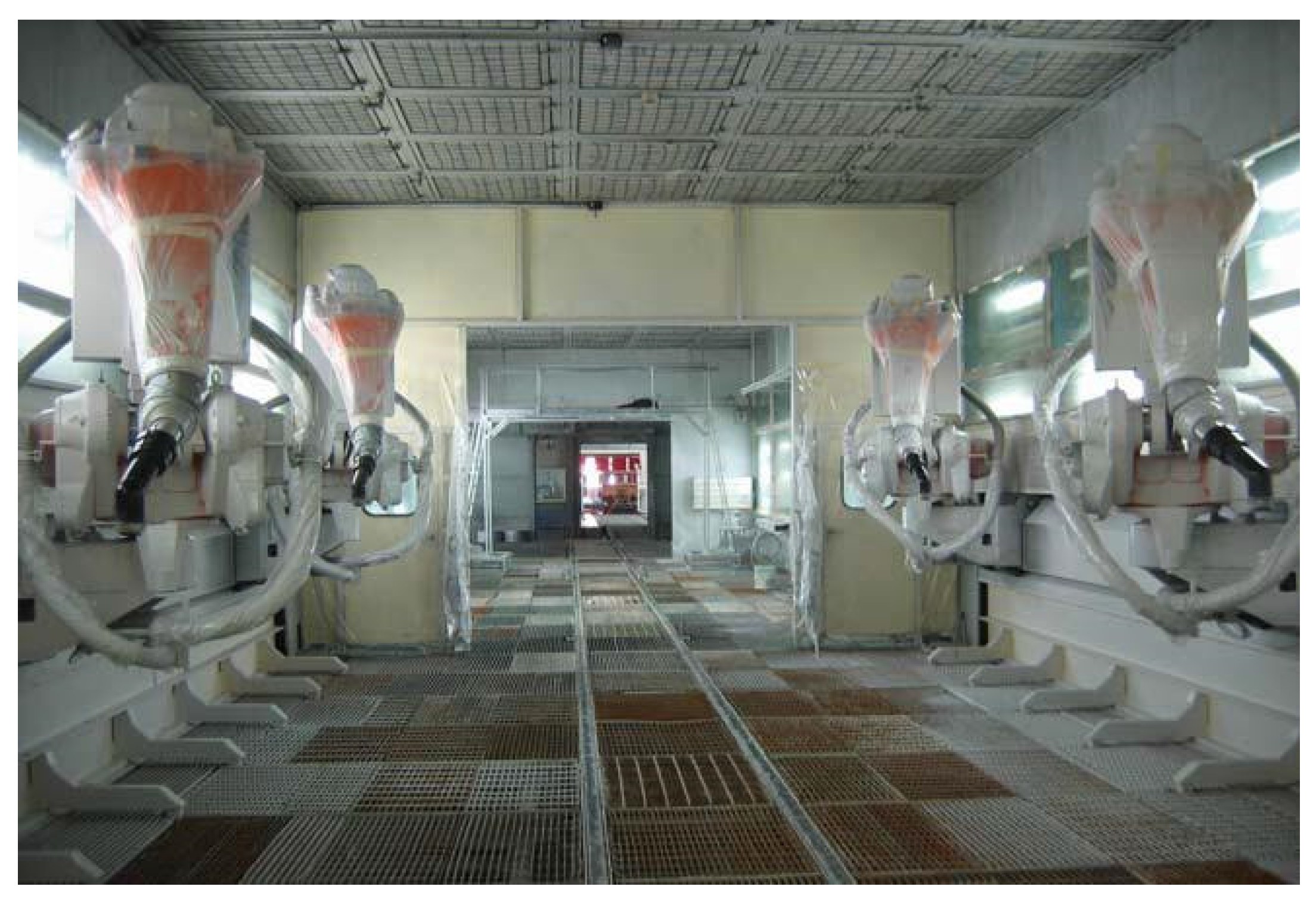
Figure 9.
Optimized trajectory of the roof.

Figure 10.
Optimized trajectory of the side.

Figure 11.
Optimized trajectory of the rear.

Figure 12.
Paint thickness at the sampling points on the automobile body.

Figure 13.
Curve of the coating thickness on the automobile body.

Figure 14.
Optimized trajectory on the roof part of the automobile.

Figure 15.
Optimized trajectory on the left and the left-rear parts of the automobile.

Figure 16.
Optimized trajectory on the right and right-rear parts of the automobile.
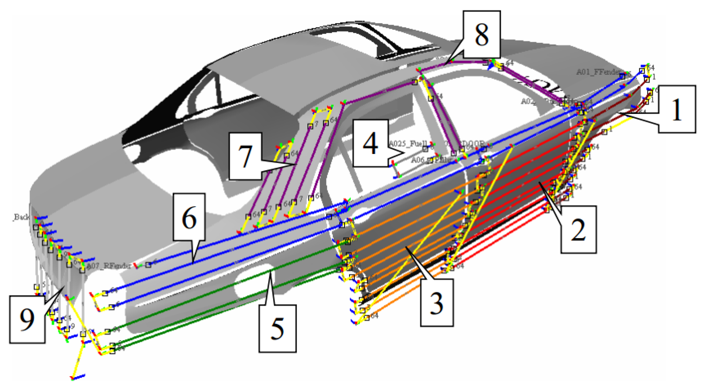
Figure 17.
Paint thickness at the sampling points on the automobile body.

Figure 18.
Curve of the coating thickness on the automobile body.

Table 1.
Operating parameters of spray trajectory on the roof.
| Trajectory | Operating Parameters of Spray Trajectory on the Roof of the Tested Automobile | |||||
|---|---|---|---|---|---|---|
| No. | Colour | Del (L/min) | AM (kRPM) | SA1 (L/min) | SA2 (L/min) | HV (kV) |
| 1 |  | 290 | 40 | 250 | 180 | 60 |
| 2 |  | 240 | 40 | 250 | 180 | 60 |
| 3 |  | 300 | 40 | 250 | 220 | 60 |
| 4 |  | 200 | 40 | 250 | 180 | 60 |
| 5 |  | 200 | 40 | 250 | 180 | 60 |
| 6 |  | 280 | 40 | 250 | 180 | 60 |
| 7 |  | 0 | 40 | 280 | 180 | 60 |
Table 2.
Operating parameters of spray trajectory on the side.
| Trajectory | Operating Parameters of Spray Trajectory on the Side of the Tested Automobile | |||||
|---|---|---|---|---|---|---|
| No. | Colour | Del (L/min) | AM (kRPM) | SA1 (L/min) | SA2 (L/min) | HV (kV) |
| 1 | | 340 | 40 | 250 | 180 | 60 |
| 2 | | 100 | 40 | 250 | 180 | 60 |
| 3 | | 310 | 40 | 250 | 180 | 60 |
| 4 | | 230 | 40 | 250 | 180 | 60 |
| 5 | | 315 | 40 | 250 | 180 | 60 |
| 6 | | 285 | 40 | 250 | 180 | 60 |
| 7 |  | 370 | 40 | 250 | 180 | 60 |
| 8 |  | 285 | 40 | 250 | 180 | 60 |
| 9 |  | 310 | 40 | 250 | 180 | 60 |
| 10 | | 350 | 40 | 350 | 250 | 60 |
| 11 | | 280 | 40 | 250 | 180 | 60 |
| 12 | | 0 | 40 | 280 | 180 | 60 |
Table 3.
Operating parameters of spray trajectory on the rear.
| Trajectory | Operating Parameters of Spray Trajectory on the Rear of the Tested Automobile | |||||
|---|---|---|---|---|---|---|
| No. | Colour | Del (L/min) | AM (kRPM) | SA1 (L/min) | SA2 (L/min) | HV (kV) |
| 1 | | 305 | 40 | 250 | 180 | 60 |
| 2 | | 295 | 40 | 250 | 180 | 60 |
| 3 | | 0 | 40 | 280 | 180 | 60 |
Table 4.
Operating parameters of the spray-painting trajectory on the roof.
| Trajectory | Operating Parameters of Spray Trajectory on the Roof of the Tested Automobile | |||||
|---|---|---|---|---|---|---|
| No. | Colour | Del (L/min) | AM (kRPM) | SA1 (L/min) | SA2 (L/min) | HV (kV) |
| 1 | | 350 | 35 | 300 | 200 | 60 |
| 2 |  | 0 | 0 | 0 | 0 | 60 |
| 3 | | 350 | 35 | 300 | 200 | 60 |
| 4 | | 350 | 35 | 300 | 200 | 60 |
Table 5.
Operating parameters of spray trajectory on the left and left-rear parts of the tested automobile.
Table 5.
Operating parameters of spray trajectory on the left and left-rear parts of the tested automobile.
| Trajectory | Operating Parameters of Spray Trajectory on the Left and Left-Rear Parts of the Tested Automobile | |||||
|---|---|---|---|---|---|---|
| No. | Colour | Del (L/min) | AM (kRPM) | SA1 (L/min) | SA2 (L/min) | HV (kV) |
| 1 | | 350 | 35 | 300 | 200 | 60 |
| 2 | | 350 | 35 | 300 | 200 | 60 |
| 3 | | 350 | 35 | 300 | 200 | 60 |
| 4 | | 0 | 0 | 0 | 0 | 60 |
| 5 | | 350 | 35 | 300 | 200 | 60 |
| 6 | | 220 | 35 | 300 | 200 | 60 |
| 7 |  | 350 | 35 | 300 | 200 | 60 |
| 8 |  | 300 | 35 | 300 | 200 | 60 |
| 9 | | 300 | 35 | 300 | 200 | 60 |
Table 6.
Operating parameters of the spray trajectory on the right and right-rear parts of the tested automobile.
Table 6.
Operating parameters of the spray trajectory on the right and right-rear parts of the tested automobile.
| Trajectory | Operating Parameters of Spray Trajectory on the Right and Right-Rear Parts of the Tested Automobile | |||||
|---|---|---|---|---|---|---|
| No. | Colour | Del (L/min) | AM (kRPM) | SA1 (L/min) | SA2 (L/min) | HV (kV) |
| 1 | | 350 | 35 | 300 | 200 | 60 |
| 2 | | 350 | 35 | 300 | 200 | 60 |
| 3 | | 350 | 35 | 300 | 200 | 60 |
| 4 | | 0 | 0 | 0 | 0 | 60 |
| 5 | | 350 | 35 | 300 | 200 | 60 |
| 6 | | 220 | 35 | 300 | 200 | 60 |
| 7 | | 350 | 35 | 300 | 200 | 60 |
| 8 | | 300 | 35 | 300 | 200 | 60 |
| 9 | | 300 | 35 | 300 | 200 | 60 |
© 2017 by the authors. Licensee MDPI, Basel, Switzerland. This article is an open access article distributed under the terms and conditions of the Creative Commons Attribution (CC BY) license (http://creativecommons.org/licenses/by/4.0/).
Share and Cite
MDPI and ACS Style
Chen, W.; Liu, H.; Tang, Y.; Liu, J. Trajectory Optimization of Electrostatic Spray Painting Robots on Curved Surface. Coatings 2017, 7, 155. https://doi.org/10.3390/coatings7100155
AMA Style
Chen W, Liu H, Tang Y, Liu J. Trajectory Optimization of Electrostatic Spray Painting Robots on Curved Surface. Coatings. 2017; 7(10):155. https://doi.org/10.3390/coatings7100155
Chicago/Turabian StyleChen, Wei, Hao Liu, Yang Tang, and Junjie Liu. 2017. "Trajectory Optimization of Electrostatic Spray Painting Robots on Curved Surface" Coatings 7, no. 10: 155. https://doi.org/10.3390/coatings7100155
Note that from the first issue of 2016, this journal uses article numbers instead of page numbers. See further details here.