1. Introduction
Over the last two decades, UV-induced Δ
n profiling in SiO
2 glasses was widely used for thw production of in-fibre/waveguide Bragg grating-based (BG) optical devices for the photonics industry. Indeed, photosensitivity allows for the fabrication of an outstanding number of in-Fiber Bragg Grating-based (FBG) optical devices like gain flattening filters (GFF), chromatic dispersion compensator (CDC) and 980 nm pump stabilization. These devices have found numerous applications in optical fiber telecommunication and all fiber laser systems. Most of these applications require long device lifetime (especially submarine optical networks) and the possibility of forecasting possible spontaneous degradation of the photo-induced index change. However, ageing experiments are always performed on a scale too short (<one month) to be extrapolated without a rational methodology. In 1998, Poumellec [
1] established a general procedure based on the existence of a demarcation energy and the notion of Master Curve (MC); what he called Variable Reaction Pathways framework or VAREPA framework. This general procedure allows to identify and to check the necessary conditions leading to a reliable prediction of various physical quantities (e.g., laser-induced refractive index changes, photodarkening, radiation induced losses in harsh environment...).
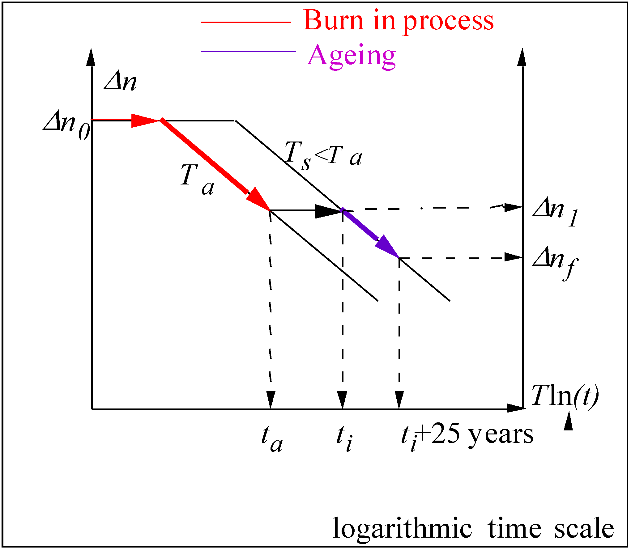
In most cases, the lifetime of a “freshly” written FBG is not large enough to satisfy the operating conditions of submarine optical networks (e.g., less than 1% decrease of the reflectivity during 25 years at 45 °C). However, the distributed nature of activation energies makes it possible to increase the grating stability by erasing thermally the less stable part of the UV-induced refractive index changes. This widespread method is called passivation process and consists in post-annealing the FBG for a time tanneal at a temperature Tanneal > Tuse. Now the question is how to perform a precise and reliable lifetime prediction of such passivated components? The usual procedure is to establish the master curve of simply outgassed components and perform the passivation FBG that have been previously out-gazed at low temperature to avoid any reactions with the remaining H2. The advantage is that this approach remains general since it can be applied to any passivation temperature provided that those are included in the master curve database and can lead to optimization of the passivation specification.
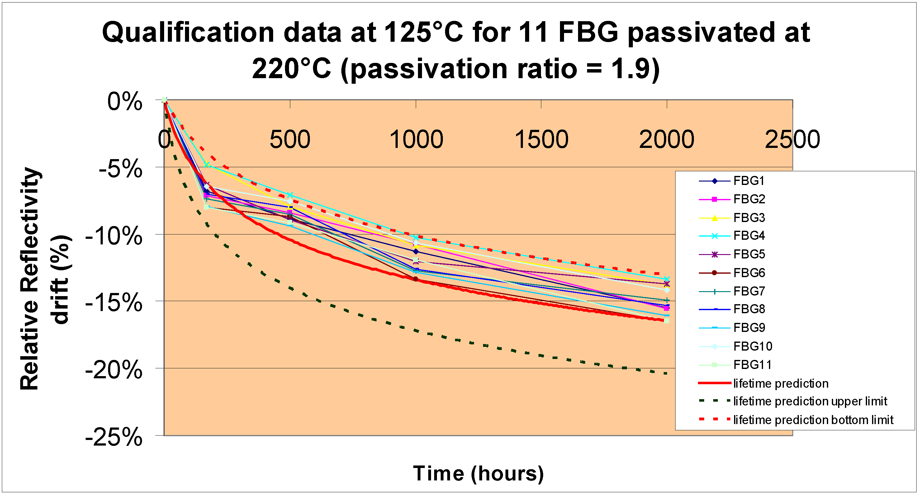
In addition, predictions must be validated. From an industrial point of view, the principle is to compare the prediction established using the MC with accelerated ageing data typically during a few 100 s of hours at a temperature higher than the working temperature, i.e., to build only one isotherm. Such an approach cannot validate the prediction in reliable manner but this is a first step and it allows the detection of potential failures in the lifetime prediction. The only right way is to build a “new” mastercurve with the real components (i.e., passivated gratings) and this is the main objective of this paper.
This approach can also be used to predict in the straight manner the lifetime of passivated components. The major advantage is to use real components (and this includes the “dispersion” of the whole manufacturing process!) resulting in a smaller lifetime prediction uncertainty. In addition, this avoids any potential failure in the predictions if the passivation conditions depart from ageing ones (e.g., presence of hydrogen during the passivation process or passivation temperature higher than the ones used during accelerated ageing).
The main objectives of this paper are thus as follows:
To quickly recall the master curve approach and related physical hypotheses
To report for the first time the passivation conditions uncertainty and their impact on the standard type I FBG lifetime prediction
To report a reliable validation procedure of the lifetime prediction. This procedure is based on building of a “new” MC derivate from real passivated gratings.
To highlight that building directly the MC on passivated FBG is less general but could be more reliable from an industrial point of view.
Below, we firstly describe FBG writing and the accelerated ageing experiments. Then we quickly recall the theory (
i.e., the VAREPA framework) that rationalizes Fiber Bragg Gratings (FBG) lifetime prediction. The main tools in this framework are the concept of demarcation energy and the master curve. Assumptions leading to their pertinence are listed. It is then shown how to obtain the master curve and the associated uncertainty from the experiments and how to determine the passivation parameters according to the lifetime specifications given by the industry. In
Section 4 we present the results for FBG dedicated to chromatic dispersion compensation,
i.e., MC building, the determination of the passivation conditions and the industrial validation procedure. Finally,
Section 5 is devoted to the uncertainty of the passivation process and we describe a reliable lifetime validation procedure.
2. FBG Writing and Accelerated Ageing Experiments
In order predict FBG lifetimes, one usually begins by measuring several quantities related to refractive index changes along the FBG during accelerated ageing experiments. They are usually reflectivity and sometimes Bragg wavelength and Bragg bandwidth. The relation between these quantities and the refractive index changes (noted RIC below) along the grating are explained in Reference [
2,
3]. Let us recall only the important features. The application of the UV light interference pattern onto the fiber material (I(
z)) during a time
tw at temperature
Tw produces a modulation of the RIC in space Δ
n(
z,
tw,
Tw) due to some physico-chemical reactions. The important features for the next discussion are 1) the mean index (Δ
nmean) which is the first component of the Fourier transform of Δ
n(
z,
tw,
Tw), 2) the refractive index modulation (Δ
nmod) at the Bragg wavelength which is the second component of the Fourier transform. Due to the linearity of the Fourier transform, the thermal stability of Δ
nmean, Δ
nmod,
i.e., (the functions Δ
nmean(
t,
T)/Δ
nmean(
tw,
Tw) and Δ
nmod(
t,
T)/Δ
nmod(
tw,
Tw)) are a weighted sum of the RIC stability at each point (
i.e., of Δ
n(
z,
t,
T)/Δ
n(
z,
tw,
Tw). In the simple case (like in slightly Ge-doped H
2-loaded fibers), the stability does not depend on the RIC amplitude at the end of the writing process (e.g., Erdogan model of electron trapping [
5]). Δ
nmean and Δ
nmod will have thus the same stability at any point of the grating and the index contrast will remain the same during the Bragg erasing. Outside of this simple case, the stability of Δ
nmean and Δ
nmod will be different.
2.1. Fiber Bragg Gratings (FBG) Writing Method and Pre-Treatments
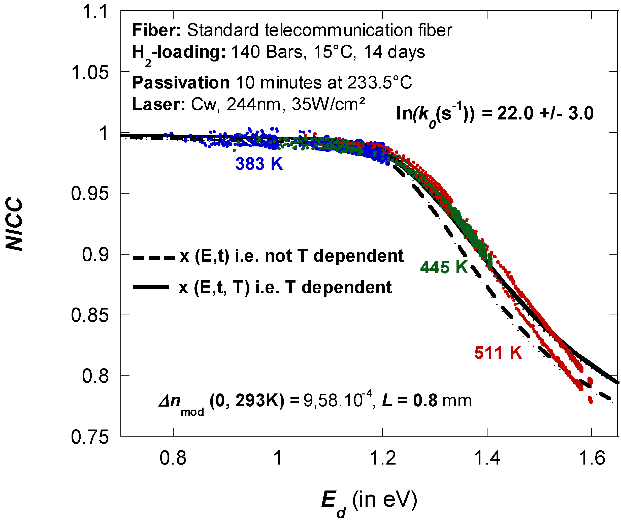
Two series of 1 mm long uniform Bragg gratings were written in H2-loaded standard telecommunication optical fibers (H2 loading conditions: 140 atm at room temperature for 15 days). To this purpose, the fibers were exposed through a phase mask (Lasiris; pitch = 1057 nm; diffraction power efficiency in the −1, +1 and 0 orders = 34%, 34% and 1% respectively) to a cw laser emitting at 244 nm. All the exposures were carried out at a mean power density ≈35 W/cm2. In this paper we will investigate two series of FBG. The first series was outgassed during 2 days at 50 °C and 2 days at 110 °C to ensure complete out-diffusion of the remaining hydrogen. The second series was first passivated during 10 min at 233 °C and then outgassed during 2 days at 50 °C and then 2 days at 110 °C to ensure complete out-diffusion of the hydrogen.
From a practical point of view, let us remind ourselves that the accelerated ageing process is applied on FBG that have been previously outgassed (i.e., we remove the H2 not consumed during FBG writing) either at room temperature (typically 1 month) or at a temperature low enough to avoid any interaction of the remaining H2 with the glass matrix (typically a 2 days below 110 °C). If the passivation process (FBG stabilization) is achieved under the same conditions than the accelerated ageing process (MC determination), it is possible then to determine its duration for a given temperature to reach a specified lifetime. Thus, to remain general (i.e., any optical fiber chemical composition and any FBG writing conditions) this approach implies to outgass the FBG before to perform the passivation. This is the usual process described in the literature. However, in many cases, industrial manufacturers will passivate FBG before H2 outgazing because it is simpler from the production point of view. In such a case, if there is a significant interaction of H2 with the glass matrix (i.e., formation an H-bearing species or transformation of existing defects that significantly impact the refractive index changes) at the passivation temperature (typically above 220 °C), the lifetime of the passivated grating cannot be deduced from the MC. In such a case it is thus necessary to build a MC direcly with the real (i.e., passivated and outgassed) components.
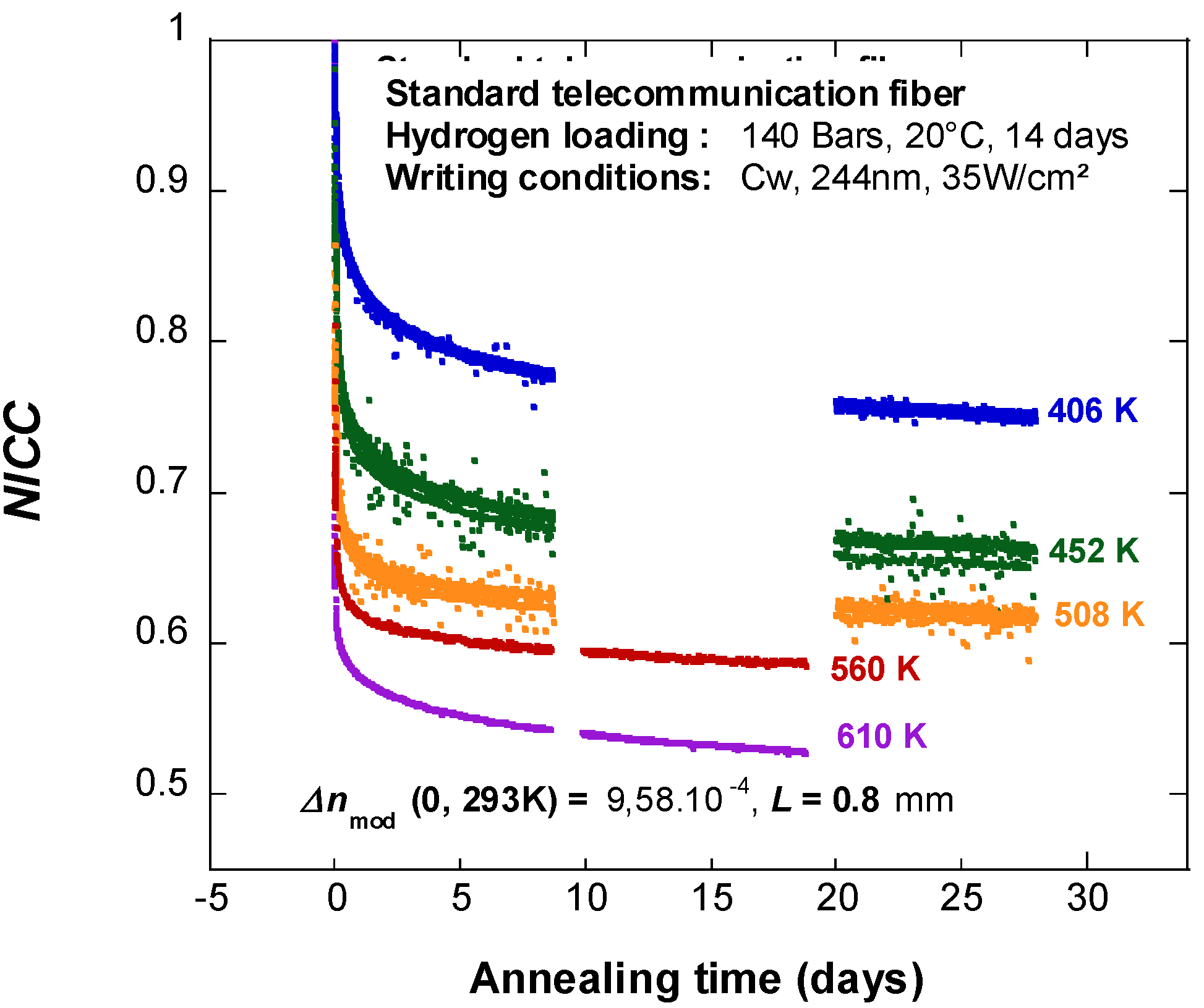
2.2. Accelerated Ageing Experiments
Three methods exist for carrying out an accelerated test. The
true isochronal annealing experiment consists in heating identical gratings at increasing temperatures for a fixed time (a new grating is used for each annealing temperature). The
step isochronal annealing is similar to the
true isochronal annealing except that the same grating is used for each annealing step. Assuming that each step is independent of the previous ones [
4], the step isochronal annealing provides a good approximation of the true isochronal annealing method [
4]. It is less time-consuming and thus it is often used. However, the preferred method usually remains to be the
isothermal annealing. It consists of holding the temperatures of identical gratings at fixed values above room temperature and periodically recording the grating transmission spectrum [
5]. This is the method that we have chosen in this study.
2.3. How to Determine the Refractive Index Decay during the Accelerated Ageing Experiments
The method consists of measuring the spectral characteristics of a uniform BG during (or after) its annealing in the single mode fiber under study. In this view, the FBG’s first-order spectra were monitored in the course of the writing and annealing experiments by means of a single-frequency tunable laser and an optical power-meter. The accuracy of the reflectivity and
λB measurements was estimated to be about 0.2% and 10 pm respectively. Then, to deduce the changes in refractive index from these data, one usually starts by assuming a step-index fiber; a periodicity of the exposure-induced change in refractive index along the fiber axis (
![Fibers 02 00092 i004]()
) and uniformity of this change across the core. The following formulae can then be used to calculate either Δ
nmod and Δ
nmean or the Normalized Integrated Coupling Constant (
NICC) from the grating reflectivity
R at
λ =
λB [
6]. Notice that those formulae are given for a simple grating [
6].
In Equation (1),
R is the grating reflectivity
Rmax at
λ = λB, T is the fixed temperature at which the BG has been held for an annealing time
t. Notice that provided the FBG is uniform and the integral overlap
η (the fraction of the total optical power propagating along the core) does not depend on
T and does not change too much during annealing,
NICC is the same quantity as the normalized modulation index:
![Fibers 02 00092 i005]()
[
2], where Δ
nmod (0,296
K) and Δ
nmod (
t,
T) are the modulation at the beginning of the annealing and after annealing at
T for
t respectively. In most experiments, both
R and
λB are measured at the temperature
T of the isothermal ageing. However, this practice can sometimes be an error source if temperature-induced reversible changes in reflectivity are not taken into account. The extent of these changes is known to be significant in some kind of FBG like non-H
2-loaded Ge-doped fibers [
7]. As these reversible changes can spoil the analysis of the isothermal annealing experiments, it proves necessary to correct the raw data to account for these changes by means of relations similar to those established in [
7]. This correction procedure will be applied in the following.
3. The Lifetime Prediction Theory: The Master Curve Formalism and the VAREPA Framework
Prediction of grating lifetime from the raw data of the isothermal annealing experiment requires an adequate kinetic model. The model is supposed to be valid beyond the time during which the ageing data have been collected (forecasting). Let us assume that this model exists. It is probably quite complex involving several physical processes [
8] and is quite uncomfortable to use. Fortunately, very often the stability can be defined by only one limiting reaction,
i.e., the one leading to the formation of the less stable chemical species (the stability of those being largely different from the other species that could contribute to the RIC). In that case, a general approach can be practiced to rationalize the FBG stability; this is the VAREPA framework including the demarcation energy and the master curve formalism. In the following paragraphs, we first describe the assumptions and how they can be validated, a necessary step in order to get confidence in the model. If the main assumptions cannot be validated, corrections can be applied at the expense of a loss of simplicity (demarcation energy approximation is conserved but MC has to be abandoned). Lastly, if no simplifying assumptions can be used, a complete kinetic model should be used.
We have also to remark that beyond the assumption of a limiting reaction, Δ
n(
z,
tw,
Tw) arises from several physical phenomena directly proportional to each other’s [
2,
3]: creation of species with a polarizability different from the non-irradiated matter polarizability, some re-organization of the matter (e.g., glass density changes) and stress redistribution. All these phenomena can thus be reduced to only one species that we will call
B in such a way that the question of stability of the RIC restricts only to the stability of
B.
(A) First group of assumptions (the application field)
(1) The first assumption we make here is that only one elementary reaction is involved: the limiting reaction of the process that makes B to disappear e.g., A←B. Note that A is not involved in the analysis.
(2) The second assumption is that it is thermally activated (with an activation energy E). The Arrhenius law can be used, the d[B]/dt rate is proportional to a reaction constant k0 like k(E, T) = k0exp(−E/kBT) where kB is the Boltzman constant and [B] is the concentration of the B species.
(3) The third assumption is that activation energy is distributed. As a matter of fact, in glasses,
E is not unique. The creation energy of
B can vary with its atomic environment. The transition state energy (the bottleneck on the reaction pathway) is also sensitive to the disordered environment in such a way that the activation energy, which is the energy difference between
B and the transition state, is distributed. The reaction pathway for erasing
B is thus variable (from where the framework has been baptized VAREPA) [
1]. Its distribution can be written
g(
E) and is normalized on the activation energy range,
i.e.,
(B) The second group of assumptions (on the reaction towards the computation of time dependence)
For computing the time and temperature dependences of the B content ([B](t, T), we have to make the following assumptions.
(1) Most of the elementary reactions in solids are first order; some are second order when two species associate but these are much less likely. So, this is not so severe and we can write:
x(
E,
t,
T) is the advancement degree of the reaction.
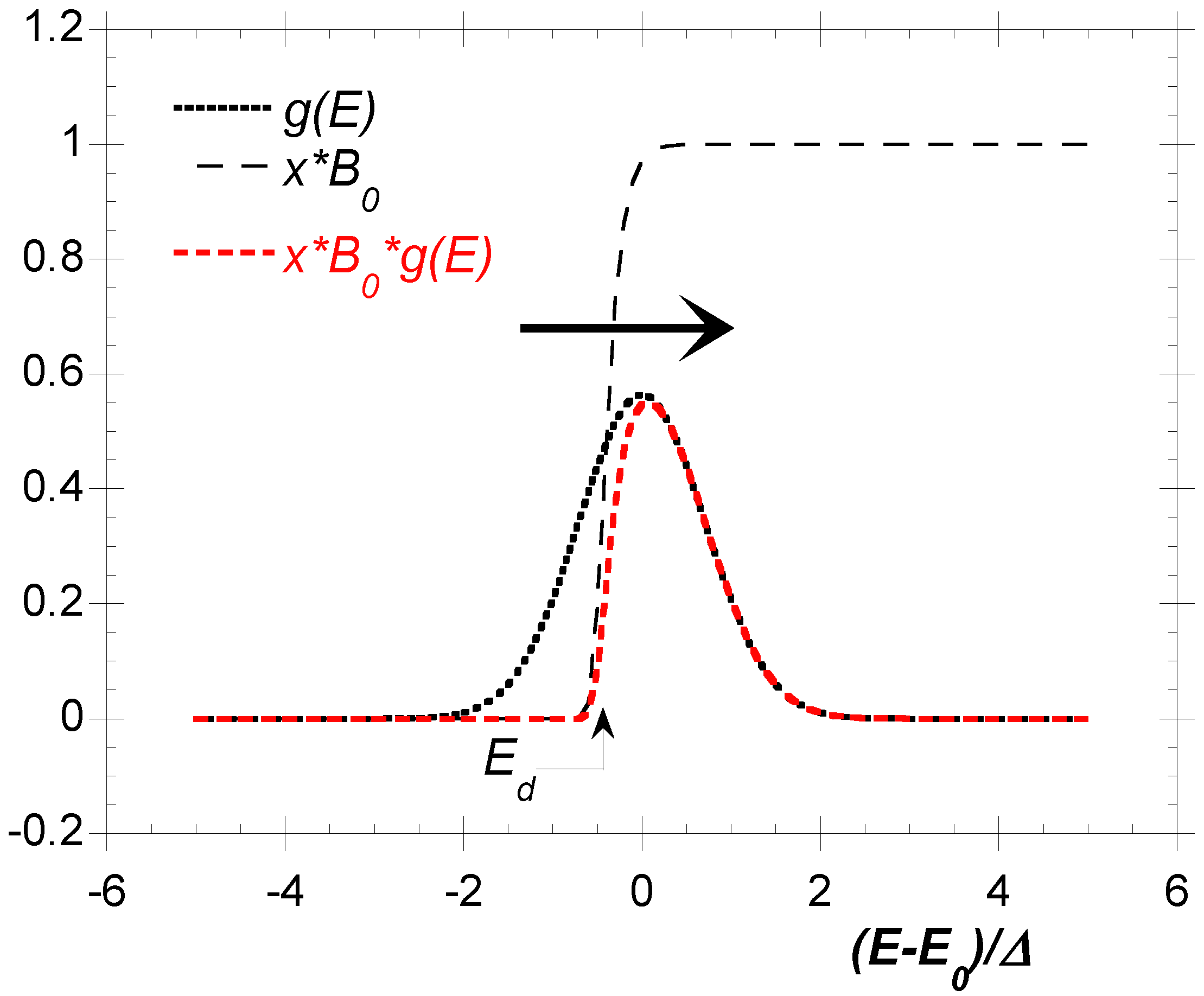
(2) Concept of demarcation energy, Ed
![Fibers 02 00092 i007]()
is a function that varies very fast with
E.
B0(
E) is the initial population produced by the FBG writing.
≥ when
x(
E,
t,
T) varies faster than
g(
E), it can be approximated to an Heaviside function at energy
Ed and thus we can read:
Ed is properly defined by
![Fibers 02 00092 i009]()
. For a first order reaction
Ed = kB.T.ln(
k0t). The reaction properties (
i.e.,
k0) are appearing in
Ed only, the disorder (relevant of the glass) appears in g(
E). Finally, [
B](
t,
T) is the area under the red dotted curve in
Figure 1. The advancement degree
x(
E,
t,
T) in progressing erases the
B distribution.
Figure 1.
Reaction progresses by erasing B sites, from less stable to the most stable sites.
Figure 1.
Reaction progresses by erasing B sites, from less stable to the most stable sites.
(C) Some consequences:
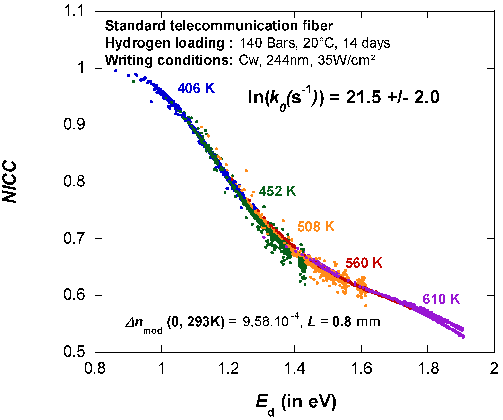
(1) [
B](
t,
T) can be expressed as a function of the unique variable called demarcation energy (
Ed). The curve [
B](
Ed) is called master curve as it is unique whatever the (
t,
T) couple may be. We can note that
T is equivalent to ln(
t) in
Ed and thus isochronal ageing data are equivalent to isothermal ageing data for establishing MC. Notice that from practical point of view most people consider that
NICC(
Ed) is the master curve. This is discussed in
Section 4. Now the MC plot allows the user to predict the grating lifetime, providing that the anticipated conditions of BG use
Ed = f(
tuse, Tuse) correspond to a point on the MC that has been actually sampled during the annealing experiment.
(2) Notice also that the distribution function is included in the MC differentiation as:
![Fibers 02 00092 i010]()


 ) and uniformity of this change across the core. The following formulae can then be used to calculate either Δnmod and Δnmean or the Normalized Integrated Coupling Constant (NICC) from the grating reflectivity R at λ = λB [6]. Notice that those formulae are given for a simple grating [6].
 [2], where Δnmod (0,296K) and Δnmod (t, T) are the modulation at the beginning of the annealing and after annealing at T for t respectively. In most experiments, both R and λB are measured at the temperature T of the isothermal ageing. However, this practice can sometimes be an error source if temperature-induced reversible changes in reflectivity are not taken into account. The extent of these changes is known to be significant in some kind of FBG like non-H2-loaded Ge-doped fibers [7]. As these reversible changes can spoil the analysis of the isothermal annealing experiments, it proves necessary to correct the raw data to account for these changes by means of relations similar to those established in [7]. This correction procedure will be applied in the following.

 is a function that varies very fast with E. B0(E) is the initial population produced by the FBG writing.

 . For a first order reaction Ed = kB.T.ln(k0t). The reaction properties (i.e., k0) are appearing in Ed only, the disorder (relevant of the glass) appears in g(E). Finally, [B](t, T) is the area under the red dotted curve in Figure 1. The advancement degree x(E, t, T) in progressing erases the B distribution.


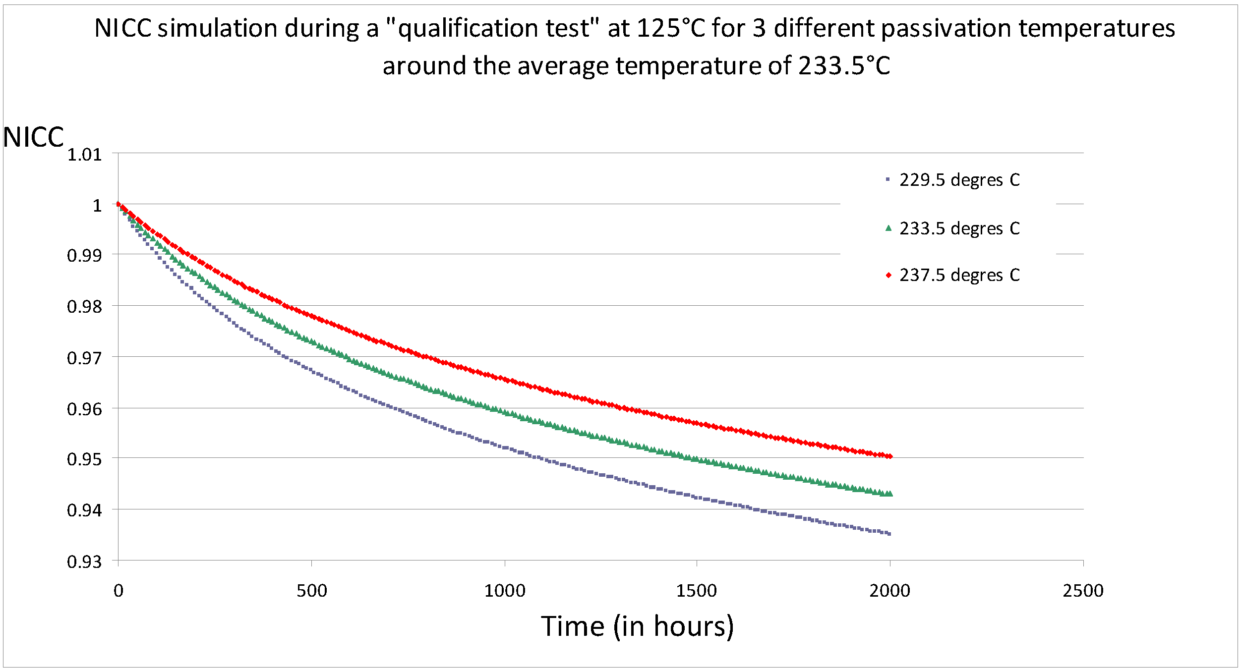
 with ε < 10% for instance, we obtain the passivation parameters (time ta and temperature Ta). Notice that in general we estimate the uncertainty on k0 based on the data uncertainty, then we chose the worst case value and we added an extra safety margin (typically ε < 1% instead of 10%).


