A Perspective on Body Size and Abundance Relationships across Ecological Communities


1
Department of Biological and Environmental Sciences and Technologies, University of Salento, Via Monteroni, Ecotekne, 73100 Lecce, Italy
2
Department of Biology, Juniata College, Huntingdon, PA 16652, USA
*
Author to whom correspondence should be addressed.
Biology 2020, 9(3), 42; https://doi.org/10.3390/biology9030042
Submission received: 11 January 2020
/
Revised: 21 February 2020
/
Accepted: 23 February 2020
/
Published: 26 February 2020
(This article belongs to the Special Issue Feature Papers 2019)
Abstract
:Recently, several studies have reported relationships between the abundance of organisms in an ecological community and their mean body size (called cross-community scaling relationships: CCSRs) that can be described by simple power functions. A primary focus of these studies has been on the scaling exponent (slope) and whether it approximates −3/4, as predicted by Damuth’s rule and the metabolic theory in ecology. However, some CCSR studies have reported scaling exponents significantly different from the theoretical value of −3/4. Why this variation occurs is still largely unknown. The purpose of our commentary is to show the value of examining both the slopes and elevations of CCSRs and how various ecological factors may affect them. As a heuristic exercise, we reanalyzed three published data sets based on phytoplankton, rodent, and macroinvertebrate assemblages that we subdivided according to three distinctly different ecological factors (i.e., climate zone, season, and trophic level). Our analyses reveal significant variation in either or both the CCSR slopes and elevations for marine phytoplankton communities across climate zones, a desert rodent community across seasons, and saltwater lagoon macroinvertebrate communities across trophic levels. We conclude that achieving a comprehensive understanding of abundance-size relationships at the community level will require consideration of both slopes and elevations of these relationships and their possible variation in different ecological contexts.
1. Introduction
Since the 1930s, researchers observed that average plant size was inversely related to population density. This density-dependent effect is observed by comparing several populations of the same species. The common occurrence of this relationship, which often shows a log-log scaling exponent of −3/2, has led to it being considered a rule or law, often called the self-thinning rule (STR), the −3/2 power rule, or Yoda’s law [1]. The STR is so general that it has even been applied to animals, though the scaling exponent may take on other values, such as −4/3. The generality of the STR has thus spurred many investigators to explain it in both plants [2,3,4] and animals (e.g., insects [5,6,7], marine invertebrates [8,9,10,11,12,13] and fish [14,15,16,17,18,19]).
Recently, the STR has also been extended to include comparisons of ecological communities of multiple species, and not just conspecific populations. Remarkably, power functions have also been successfully applied at the community level, thus starting a new wave of analyses of cross-community scaling relationships (CCSR). CCSRs describe negative relationships between the total number or density of organisms in an assemblage or community of species and their average body size [20]. These relationships are often so regular that they can be described by the power function:
where N is population density, k is a normalization constant, B is individual body mass, and b is the scaling exponent. According to Damuth’s Rule, which is based on comparisons of species populations, the scaling exponent should be −3/4 [21,22,23,24]. The ‘metabolic theory of ecology’ makes a similar prediction, by assuming that the scaling exponent for population density should be the inverse of that based on the 3/4-power law for metabolic rate [25]. This assumption derives from the Energetic Equivalence Rule (EER), which posits that species populations use approximately the same amount of energy regardless of body size (calculated as energetic demand per individual, scaled to body mass according to the 3/4-power law, times the number of individuals in a population [23,24]).
N = kBb,
However, when ecological densities are compared among community assemblages of closely related species, the slope of the CCSR may deviate from the theoretical value of −3/4. These deviations may occur if the EER is not obeyed. For example, a less steep slope may occur if large species acquire more energy than smaller species. In contrast, a steeper slope may occur if small species acquire more energy than larger species [21,22,23]. These deviations from that expected by the EER or MTE show that the amount of energy used is not the same for all species, which may result from the effects of various biotic and abiotic environmental factors.
To date, several studies of CCSRs have been carried out on diverse assemblages of plants [26], phytoplankton [27], bacteria, algae and protozoa [20,28], fish, amphibians and macroinvertebrates [29,30,31,32], birds [33], and rodents [34]. However, the focus of these studies has been chiefly on the scaling exponent and whether it matches the theoretically predicted value of −3/4. In this commentary, we advocate expanding the focus of studies of CCSRs to include explorations of the biological meaning of both their slopes and elevations, especially in relation to various intrinsic (biological) and extrinsic (ecological) factors. We support this view by re-analyzing selected data sets from previously published papers to show that either the slopes or elevations (or both) of CCSRs vary considerably in relation to three distinctly different ecological factors: climate zone, season and trophic level. The results of our heuristic exercise add to the growing literature showing that diverse kinds of biological and ecological scaling relationships do not necessarily follow simple universal laws, but vary substantially in relation to various biological and ecological contexts (e.g., [35,36,37,38,39,40]).
2. Case Studies
2.1. Across Climate Zones (Biogeographic Regions)
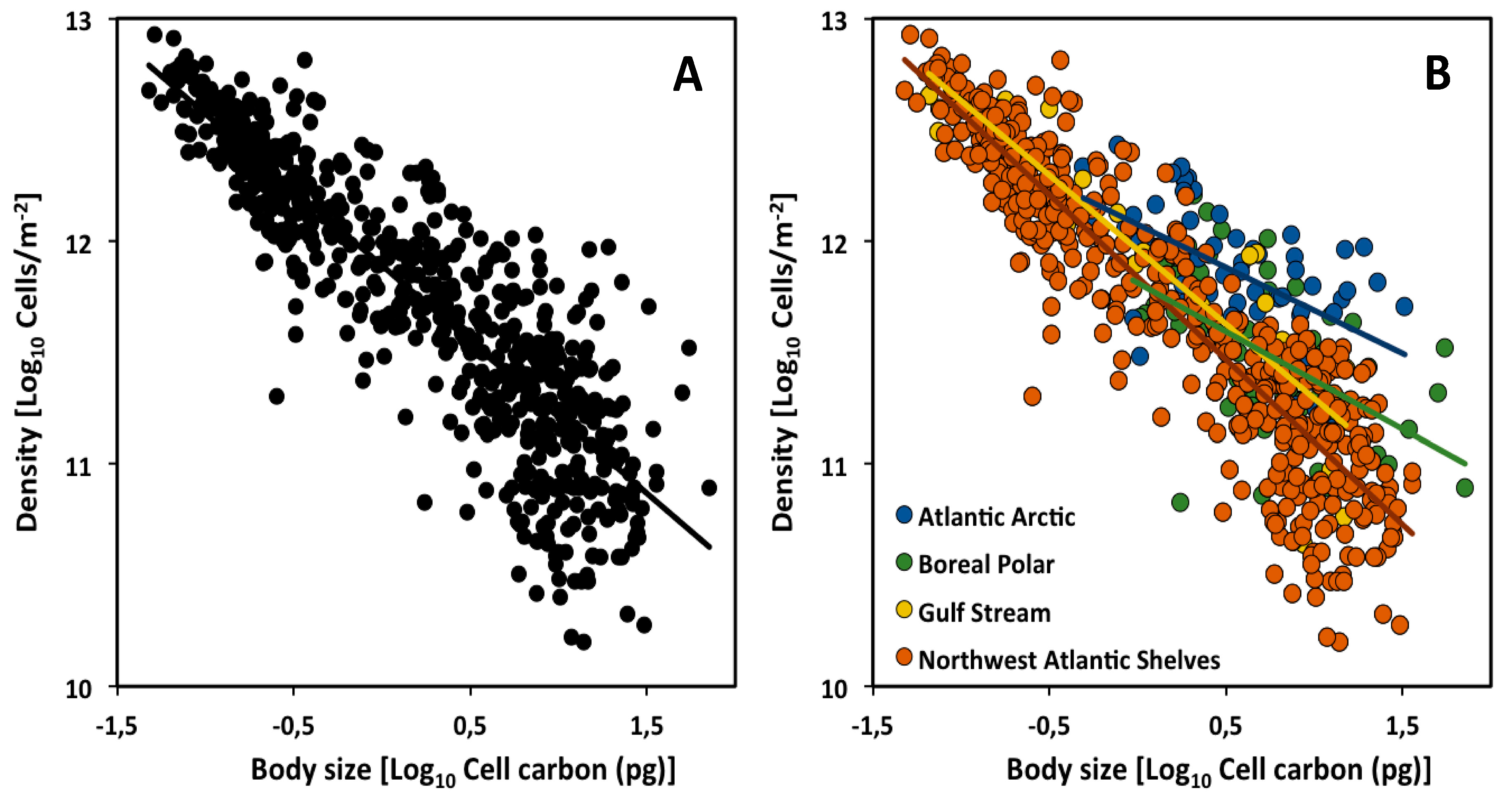
The scaling slope for the CCSR of 635 marine phytoplankton community assemblages in the Northern Hemisphere of the Atlantic Ocean was found to be −0.78 (95% confidence interval = −0.74 to −0.81, based on reduced major axis (Model II) regression; Figure 1A), which does not differ significantly from the theoretical value of −3/4 [27]. This analysis and other phytoplankton studies [4,41] support the generality of the −3/4-power rule of Damuth and the MTE (but note that a least squares (Model I) regression (LSR) analysis of the data of [27] yields an exponent (−0.68: Table 1) significantly less than −3/4). However, plankton communities consisting of both phyto- and zooplankton show CCSR scaling exponents of −1, apparently resulting from a dominance of small-sized species [42]. Here we show that the CCSR scaling exponent may vary not only with plankton species composition, but also with climate zone or biogeographic region.
We divided the dataset of [27] according to four climate zones. Our LSR analyses show that the CCSR exponents and intercepts for cell density versus mean cell size (carbon content) vary significantly across the four climate zones (Figure 1B). In particular, although the slopes are not significantly different from −3/4 in the assemblages occupying the southern climate zones (Gulf Stream and Northwest Atlantic Shelves), they are significantly lower than −3/4 in the assemblages occupying the northern climate zones (Atlantic Arctic and Boreal Polar) (see Table 1, Figure 1B).
Furthermore, size-specific cell densities (and thus overall scaling elevations) tend to be higher in the northern vs. southern climate zones (ANCOVA analysis comparing 95% confidence interval; Table 2). This could be explained hypothetically as the result of two major influences: larger cells are favored in colder more northerly climate zones (following the temperature size rule, as the data seem to show) and lower temperatures cause lower metabolic (nutrient) demand per cell, thus enabling higher total cell densities [43,44,45].
This hypothesis may also help explain why the scaling slopes of the CCSRs are lower in the northern versus southern climate zones. This difference may arise because although small-celled species show similar densities in all climate zones, larger-celled species show significantly higher densities in northern vs. southern climate zones. This may be because much fewer small-celled species occur in the northern climate zones, thus freeing up resources (nutrients) for larger-celled species that can then build up higher densities. However, many small-celled species occur in the southern climate zones, and their competitive exploitation of shared nutrients limits the densities of larger-celled species to lower levels. In short, a shift in competitive advantage from small to large cells with increasing latitude and decreasing temperature may cause changes in both the scaling slopes and elevations of the CCSRs observed.
2.2. Across Seasons
The CCSR of a desert rodent community also shows an exponent not significantly different from the theoretical value of −3/4 [34]. LSR analysis of overall abundance with mean body size at the same sampling site in Portal Arizona over a 25-year period (1987 to 2002), showed a CCSR exponent of −0.57 (n = 25, 95% confidence interval: −0.97 to −0.18). The CCSR was constructed from community assemblages at different time periods (rather than different spatial locations, as typically done). Each data point was based on monthly sampling during a specific year, which was performed three or four times. However, the data set includes only the species that occurred during a 6-month period in at least five years during the 25 years period of the data set.
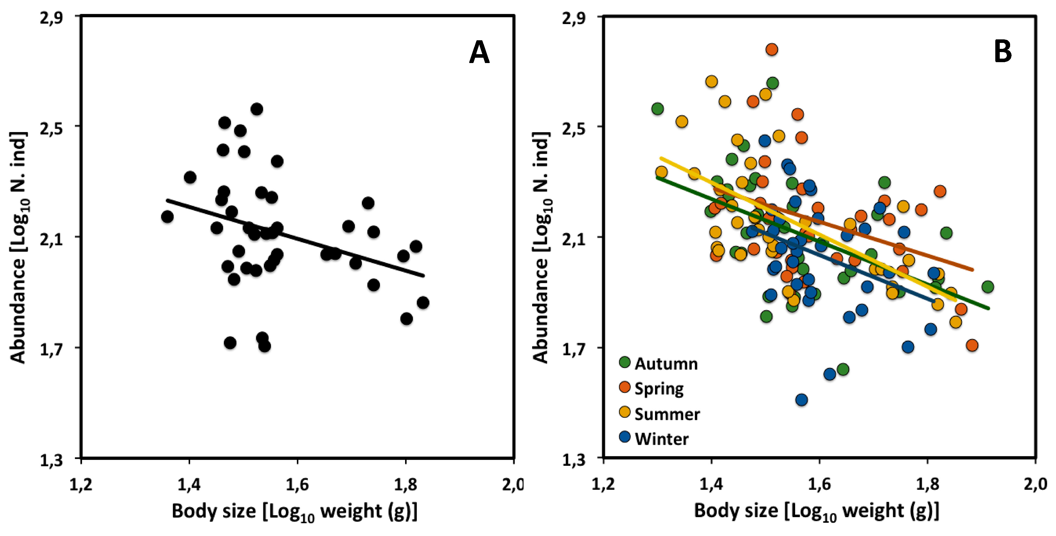
We obtained an updated data set covering 41 years of sampling, kindly provided by Ethan White, and divided it according to season. Our LSR analysis of this dataset, including all species sampled, yielded a CCSR scaling exponent similar to that found over the 25-year period analyzed by [34], and not significantly different from the theoretical value of −3/4 (Table 3, Figure 2A). Moreover, the CCSR scaling exponents for each of the four seasons did not differ significantly from each other (Table 3, Figure 2B), nor with −3/4. However, the CCSR elevation was significantly higher during the spring than during the winter (ANCOVA analysis comparing 95% confidence interval; Table 4).
Rodents may have reached their highest density during spring, because this is when reproduction and the appearance of juveniles tend to peak for most species [46,47,48]. However, during the winter, density is relatively low because breeding is low, thus causing a net loss of individuals by mortality. The relative heights of the elevations of these relationships are consistent with the proposed hypothesis. As shown in Figure 2B, rodent densities tended to be lowest during winter, rising to the highest level during spring, and then declining again through summer and autumn. Therefore, our analysis suggests that although the energy flow of the desert rodent community has apparently not changed over the 25-year period studied by [34], it has changed seasonally during each year (as indicated by seasonal changes in the scaling elevation for population density).
2.3. Across Trophic Levels
Although some CCSR scaling exponents reported in the literature so far are not significantly different from the theoretical value of −3/4 ([27,32,33,34]; see also Section 3), a recent analysis of 158 aquatic macroinvertebrate community assemblages has revealed an exponent significantly lower than −3/4 (−0.27, 95% confidence interval = −0.411 to −0.131) [29]. This data set included spring and summer samples from saltwater lagoons in the biogeographic regions of the Eastern Mediterranean Sea and the Black Sea. It suggests that large macroinvertebrate species seem to be acquiring more energy than smaller species.
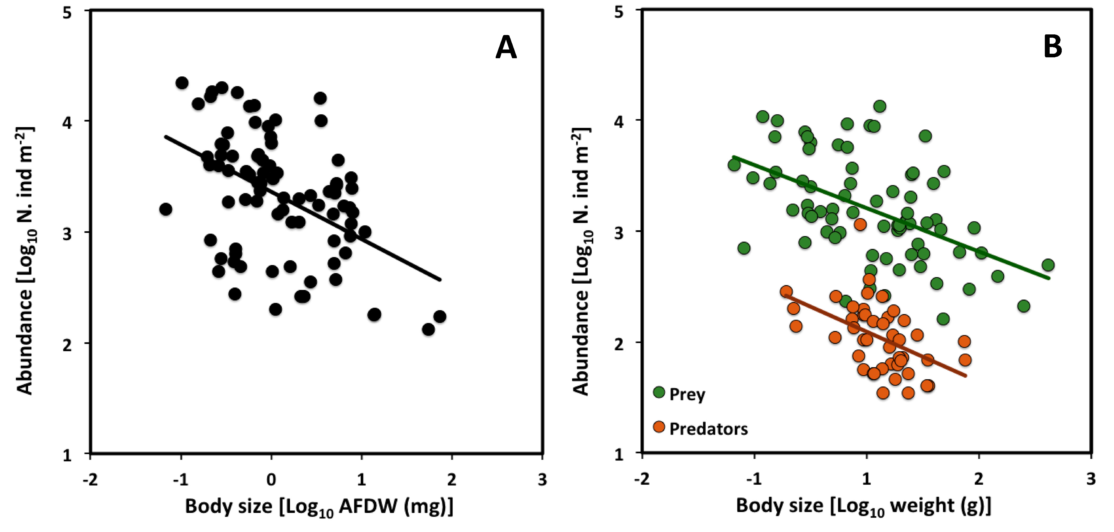
We reanalyzed the data set of [29] by averaging the data for spring and autumn. Again, the CCSR scaling exponent (−0.43) is not significantly different from the value obtained by [29], and is still significantly lower than −3/4 (Table 5, Figure 3A). Furthermore, after separating the data by trophic level, the CCSR scaling exponent is significantly lower than −3/4 for predator and prey species analyzed separately (−0.45 and −0.39, respectively: see Table 5, Figure 3B). However, the elevation of the scaling relationship is significantly higher for prey than predators (ANCOVA analysis comparing 95% confidence intervals; Table 6).
The higher CCSR elevation for prey vs. predators may be explained in terms of both general theory and observations specific to saltwater lagoons. Following the second law of thermodynamics, as energy is transformed from lower to higher trophic levels in a food web, much energy is lost as heat [49,50]. Therefore, since prey tend to have more energy available to them than predators that feed upon them, they can also sustain higher population densities at equivalent body sizes. In addition, macroinvertebrate prey in shallow, highly productive, saltwater lagoons are mainly detritus and suspension feeders. The energy available to them from abundant, easily acquired detritus and fine organic matter in the water column and at the bottom of lagoons is much more abundant than that available to predators that feed chiefly on animal tissue, which is more difficult to acquire [51,52,53]. Our results are consistent with previous findings showing that prey tend to have higher population abundances than that of predators, even if predators affect the abundance of prey [54,55,56,57,58].
3. Discussion
Most previous studies of abundance-size relationships across ecological communities have focused on the scaling exponent, and whether it is similar to the −3/4 values predicted by Damuth’s rule and the MTE [21,22,23,24,25]. Although three major studies have yielded CCSR exponents not significantly different from −3/4, three other studies have reported exponents significantly higher or lower than −3/4 (Table 7). Why this is so is still little understood. Some of this variation may relate to taxonomic and/or environmental differences.
In our commentary, we suggest that better understanding of CCSRs may be achieved by examining both the slopes and elevations of these relationships, and how they are affected by various ecological factors. To support this point, we reanalyzed three data sets published in the literature. Instead of examining these data sets as a whole, as done by the original authors, we divided them using various ecological factors, including climate zone, season and trophic level. In all of our case studies, we found significant variation in CCSR slopes and/or elevations (intercepts) among our ecologically classified subsamples.
First, we found significant differences in slopes and elevations between CCSRs of marine phytoplankton communities from northern cold climate zones versus southern warmer climate zones that could be explained in terms of plausible temperature effects on the cell size, metabolic rate and density of phytoplankton (Section 2.1). Second, we discovered significant seasonal differences in the elevations of CCSRs based on temporal samples of a desert rodent community that could be explained as a result of seasonal differences in offspring production (Section 2.2). Third, we found significant differences in the elevations of CCSRs for prey versus predators of saltwater lagoon macroinvertebrate communities that could be explained by lower availability of energy at higher trophic levels (Section 2.3).
All of these case studies reveal the value of subdividing ecologically heterogeneous data sets into more homogeneous ecological categories. By doing so, significant differences in CCSRs may be found that can help elucidate the mechanisms underlying them. Our analyses also reveal the importance of exploring the biological meaning of both the slopes and elevations of CCSRs, as recommended in general for allometric scaling analyses (e.g., [35,36,59,60]).
4. Conclusions
Although abundance−size relationships have received much attention by ecologists at the population level, little is known about these relationships at the community level. We hope that our analyses will serve as heuristic examples that will motivate other researchers to explore ecological and taxonomic effects on both the slopes and elevations of CCSRs. Although universal laws are useful for testing theoretical expectations on major ecological issues, various contingent factors may cause many kinds of biological and ecological scaling relationships to deviate from universal laws [34,35,36,37,38,39,40]. We suggest that the search for and understanding of regular patterns in nature benefit from not only employing general theories based on single, hypothetically universal, deterministic mechanisms, but also an awareness that multiple contingent mechanisms that vary with biological and ecological context may underlie the diversity that we often see.
Author Contributions
Conceptualization, V.G., D.S.G.; methodology, V.G., D.S.G.; formal analysis, V.G.; investigation, V.G., D.S.G., resources, V.G., D.S.G.; data curation, V.G.; writing—original draft preparation, V.G., D.S.G.; writing—review and editing, V.G., D.S.G.; visualization, V.G., D.S.G.; supervision, V.G., D.S.G.; project administration, V.G., D.S.G.; funding acquisition, V.G., D.S.G. All authors have read and agreed to the published version of the manuscript.
Funding
This research was funded by a Brusarosco grant from the Italian Society of Ecology (SItE) awarded to Vojsava Gjoni in support of her research visit at Juniata College.
Acknowledgments
We thank E.P. White and W.K.W. Li for providing and sharing data sets on rodents and phytoplankton assemblages, respectively. We also thank the anonymous reviewers for their helpful comments.
Conflicts of Interest
The authors declare no conflict of interest. The funders had no role in the design of the study; in the collection, analyses, or interpretation of data; in the writing of the manuscript, or in the decision to publish the results.
Appendix A
In order to minimize stochastic effects on the size−abundance relationship of the desert rodent community analyzed by [34], we removed 3 years (i.e., 1993, 1994, 2010) of the original data that included too low densities of rodents. These 3 years showed from 51 to 54 individuals averaging per month all the seasons. However, dividing into the four seasons and averaging per month each season, the lower number of the individuals reaches 27 individuals. This reduced data set was considered for all subsequent LSR analyses of the CCSRs on the rodent communities across seasons.
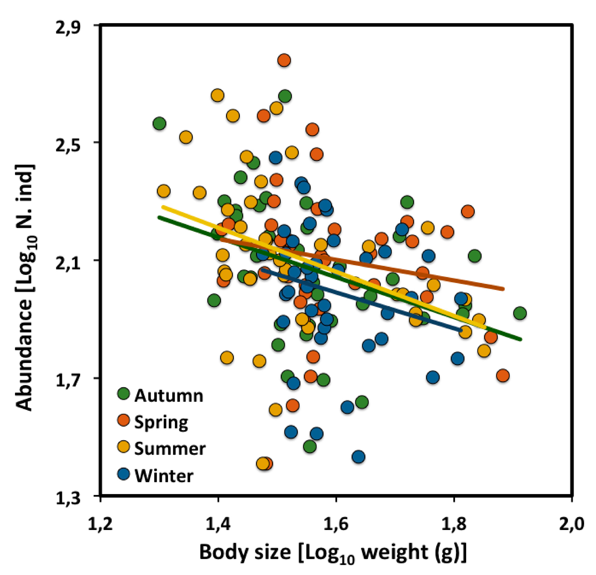
Figure A1.
Scaling of density versus mean body size (live weight) of a desert rodent community in Portal Arizona through 41 years, from 1978 to 2018 (data from [34]) across the four seasons.
Figure A1.
Scaling of density versus mean body size (live weight) of a desert rodent community in Portal Arizona through 41 years, from 1978 to 2018 (data from [34]) across the four seasons.

Here, we show the LSR analyses of the rodent community CCSRs based on all of the years of the original data set. In this case, the only significant difference that was observed was a scaling exponent of −0.35 for the spring samples, which was significantly lower than −3/4 and that observed for samples taken during the other three seasons (Table A1, Figure A1). The scaling exponents for the autumn, summer and winter samples were not significantly different as well from the theoretical value of −3/4. The elevations among the four seasons were not significantly different because of the high variation and the wide range of the 95% confidence interval of all four CCSRs (ANCOVA analysis comparing 95% confidence interval; Table A2).

Table A1.
Results of LSR analyses of log10 population abundance (number of individuals) in relation to log10 body size (mg) of a desert rodent community in Portal Arizona (updated data from [34]).
Table A1.
Results of LSR analyses of log10 population abundance (number of individuals) in relation to log10 body size (mg) of a desert rodent community in Portal Arizona (updated data from [34]).
| CCSR | Slope | Intercept | 95% CI | n | r2 | p |
|---|---|---|---|---|---|---|
| Autumn | −0.71 | 3.18 | −1.27 to −0.15 | 41 | 0.15 | * |
| Spring | −0.35 | 2.67 | −1.05 to −0.34 | 41 | 0.03 | ns |
| Summer | −0.75 | 3.26 | −1.28 to −0.22 | 41 | 0.17 | ** |
| Winter | −0.61 | 2.97 | −1.47 to −0.25 | 41 | 0.05 | ns |
* p < 0.05; ** p < 0.005; ns—not significant.
Table A2.
p values for slope and intercept comparisons of the LSR analyses in Table A1. The differences among slopes were assessed by comparing 95% CI. When the slopes were not significantly different, the differences between elevations were estimated by ANCOVA (with body mass as a covariate).
Table A2.
p values for slope and intercept comparisons of the LSR analyses in Table A1. The differences among slopes were assessed by comparing 95% CI. When the slopes were not significantly different, the differences between elevations were estimated by ANCOVA (with body mass as a covariate).
| Seasons | p Value for Slope a | p Value for Intercept b | ||||||
|---|---|---|---|---|---|---|---|---|
| AU | SP | SU | WI | AU | SP | SU | WI | |
| Autumn (AU) | - | ns | ns | ns | - | ns | ns | ns |
| Spring (SP) | ns | - | ns | ns | ns | - | ns | ns |
| Summer (SU) | ns | ns | - | ns | ns | ns | - | ns |
| Winter (WI) | ns | ns | ns | - | ns | ns | ns | - |
a Significance of slope differences; b Significance of intercept differences; ns—not significant; - not measurable.
References
- Li, B.L.; Wu, H.I.; Zou, G. Self-thinning rule: A causal interpretation from ecological field theory. Ecol. Model. 2000, 132, 167–173. [Google Scholar] [CrossRef]
- Yoda, K. Self-thinning in overcrowded pure stands under cultivated and natural conditions (Intraspecific competition among higher plants. XI). J. Inst. Polytech. Osaka City Univ. 1963, 14, 107–129. [Google Scholar]
- Westoby, M. The place of the self-thinning rule in population dynamics. Am. Nat. 1981, 118, 581–587. [Google Scholar] [CrossRef]
- Belgrano, A.; Allen, A.P.; Enquist, B.J.; Gillooly, J.F. Allometric scaling of maximum population density: A common rule for marine phytoplankton and terrestrial plants. Ecol. Lett. 2002, 5, 611–613. [Google Scholar] [CrossRef]
- Begon, M.; Firbank, L.; Wall, R. Is there a self-thinning rule for animal populations? Oikos 1986, 46, 122–124. [Google Scholar] [CrossRef]
- Latto, J. Evidence for a self-thinning rule in animals. Oikos 1994, 69, 531–534. [Google Scholar] [CrossRef]
- Fréchette, M.; Lefaivre, D. On self-thinning in animals. Oikos 1995, 73, 425–428. [Google Scholar] [CrossRef]
- Branch, G.M. Mechanisms reducing intraspecific competition in Patella spp.: Migration, differentiation and territorial behaviour. J. Anim. Ecol. 1975, 44, 575–600. [Google Scholar] [CrossRef]
- Hogarth, P.J. Population Density, Mean Weight, and the Nature of the “Thinning Line” in Semibalanus balanoides (L.) (Cirripedia Thoracica). Crustaceana 1985, 49, 215–218. [Google Scholar] [CrossRef]
- Hughes, R.N.; Griffiths, C.L. Self-thinning in barnacles and mussels: The geometry of packing. Am. Nat. 1988, 132, 484–491. [Google Scholar] [CrossRef]
- Frechette, M.; Lefaivre, D. Discriminating between food and space limitation in benthic suspension feeders using self-thinning relationships. Mar. Ecol. Prog. Ser. 1990, 65, 15–23. [Google Scholar] [CrossRef]
- Petraitis, P.S. The role of growth in maintaining spatial dominance by mussels (Mytilus edulis). Ecology 1995, 76, 1337–1346. [Google Scholar] [CrossRef]
- Guinez, R.; Castilla, J.C. A tridimensional self-thinning model for multilayered intertidal mussels. Am. Nat. 1999, 154, 341–357. [Google Scholar] [CrossRef] [PubMed]
- Grant, J.W.; Kramer, D.L. Territory size as a predictor of the upper limit to population density of juvenile salmonids in streams. Can. J. Fish. Aquat. Sci. 1990, 47, 1724–1737. [Google Scholar] [CrossRef]
- Elliott, J.M. The self-thinning rule applied to juvenile sea trout, Salmo trutta. J. Anim. Ecol. 1993, 62, 371–379. [Google Scholar] [CrossRef]
- Bohlin, T.; Dellefors, C.; Faremo, U.; Johlander, A. The energetic equivalence hypothesis and the relation between population density and body size in stream-living salmonids. Am. Nat. 1994, 143, 478–493. [Google Scholar] [CrossRef]
- Armstrong, J.D.; Herbert, N.A. Homing movements of displaced stream-dwelling brown trout. J. Fish Biol. 1997, 50, 445–449. [Google Scholar] [CrossRef]
- Dunham, J.B.; Vinyard, G.L. Relationships between body mass, population density, and the self-thinning rule in stream-living salmonids. Can. J. Fish. Aquat. Sci. 1997, 54, 1025–1030. [Google Scholar] [CrossRef]
- White, E.P.; Ernest, S.M.; Kerkhoff, A.J.; Enquist, B.J. Relationships between body size and abundance in ecology. Trends Ecol. Evol. 2007, 22, 323–330. [Google Scholar] [CrossRef] [Green Version]
- Damuth, J.D. Population density and body size in mammals. Nature 1981, 290, 699–700. [Google Scholar] [CrossRef]
- Damuth, J.D. Of size and abundance. Nature 1991, 351, 268–269. [Google Scholar] [CrossRef]
- Damuth, J.D. Population ecology: Common rules for animals and plants. Nature 1998, 395, 115–116. [Google Scholar] [CrossRef]
- Nee, S.; Read, A.F.; Greenwood, J.J.; Harvey, P.H. The relationship between abundance and body size in British birds. Nature 1991, 351, 312–313. [Google Scholar] [CrossRef]
- Brown, J.H.; Gillooly, J.F.; Allen, A.P.; Savage, V.M.; West, G.B. Toward a metabolic theory of ecology. Ecology 2004, 85, 1771–1789. [Google Scholar] [CrossRef]
- Enquist, B.J.; Brown, J.H.; West, G.B. Allometric scaling of plant energetics and population density. Nature 1998, 395, 163–165. [Google Scholar] [CrossRef]
- Li, W.K.W. Macroecological patterns of phytoplankton in the northwestern North Atlantic Ocean. Nature 2002, 419, 154–157. [Google Scholar] [CrossRef]
- Long, Z.T.; Morin, P.J. Effects of organism size and community composition on ecosystem functioning. Ecol. Lett. 2005, 8, 1271–1282. [Google Scholar] [CrossRef]
- Gjoni, V.; Cozzoli, F.; Rosati, I.; Basset, A. Size-density relationships: A cross-community approach to benthic macroinvertebrates in Mediterranean and Black Sea lagoons. Estuar. Coast. 2017, 40, 1142–1158. [Google Scholar] [CrossRef]
- Gjoni, V.; Basset, A. A cross-community approach to energy pathways across lagoon macroinvertebrate guilds. Estuar. Coast. 2018, 41, 2433–2446. [Google Scholar] [CrossRef]
- Gjoni, V.; Ghinis, S.; Pinna, M.; Mazzotta, L.; Marini, G.; Ciotti, M.; Rosati, I.; Vignes, F.; Arima, S.; Basset, A. Patterns of functional diversity of macroinvertebrates across three aquatic ecosystem types, NE Mediterranean. Mediterr. Mar. Sci. 2019, 20, 703–717. [Google Scholar] [CrossRef] [Green Version]
- Arim, M.; Berazategui, M.; Barreneche, J.M.; Ziegler, L.; Zarucki, M.; Abades, S.R. Determinants of density–body size scaling within food webs and tools for their detection. Adv. Ecol. Res. 2011, 45, 1–39. [Google Scholar]
- Meehan, T.D.; Jetz, W.; Brown, J.H. Energetic determinants of abundance in winter landbird communities. Ecol. Lett. 2004, 7, 532–537. [Google Scholar] [CrossRef]
- White, E.P.; Ernest, S.M.; Thibault, K.M. Trade-offs in community properties through time in a desert rodent community. Am. Nat. 2004, 164, 670–676. [Google Scholar] [CrossRef]
- Glazier, D.S. Beyond the ‘3/4−power law’: Variation in the intra−and interspecific scaling of metabolic rate in animals. Biol. Rev. 2005, 80, 611–662. [Google Scholar] [CrossRef] [PubMed]
- Glazier, D.S. A unifying explanation for diverse metabolic scaling in animals and plants. Biol. Rev. 2010, 85, 111–138. [Google Scholar] [CrossRef] [PubMed]
- Glazier, D.S. Metabolic scaling in complex living systems. Systems 2014, 2, 451–540. [Google Scholar] [CrossRef] [Green Version]
- Glazier, D.S. Rediscovering and reviving old observations and explanations of metabolic scaling in living systems. Systems 2018, 6, 4. [Google Scholar] [CrossRef] [Green Version]
- Griffen, B.D.; Cannizzo, Z.J.; Gül, M.R. Ecological and evolutionary implications of allometric growth in stomach size of brachyuran crabs. PLoS ONE 2018, 13, e0207416. [Google Scholar] [CrossRef] [Green Version]
- Malerba, M.E.; Marshall, D.J. Size-abundance rules? Evolution changes scaling relationships between size, metabolism and demography. Ecol. Lett. 2019, 22, 1407–1416. [Google Scholar] [CrossRef]
- Agusti, S.; Kalff, J. The influence of growth conditions on the size dependence of maximal algal density and biomass. Limnol. Oceanogr. 1989, 34, 1104–1108. [Google Scholar] [CrossRef]
- Rodríguez, J. Some comments on the size-based structural analysis of the pelagic ecosystem. Sci. Mar. 1994, 58, 1–10. [Google Scholar]
- Li, W.K.W.; Glen Harrison, W.; Head, E.J. Coherent assembly of phytoplankton communities in diverse temperate ocean ecosystems. Proc. R. Soc. B−Biol. Sci. 2006, 273, 1953–1960. [Google Scholar] [CrossRef] [Green Version]
- Atkinson, D. Effects of temperature on the size of aquatic ectotherms: Exceptions to the general rule. J. Therm. Biol. 1995, 20, 61–74. [Google Scholar] [CrossRef]
- Atkinson, D.; Ciotti, B.J.; Montagnes, D.J.X. Protists decrease in size linearly with temperature: Ca. 2.5% C− 1. Proc. R. Soc. B−Biol. Sci. 2003, 270, 2605–2611. [Google Scholar] [CrossRef] [Green Version]
- Morán, X.A.G.; López-Urrutia, Á.; Calvo-Díaz, A.; Li, W.K.W. Increasing importance of small phytoplankton in a warmer ocean. Glob. Chang. Biol. 2010, 16, 1137–1144. [Google Scholar] [CrossRef]
- Kenagy, G.J.; Bartholomew, G.A. Seasonal reproductive patterns in five coexisting California desert rodent species. Ecol. Monogr. 1985, 55, 371–397. [Google Scholar] [CrossRef]
- Zeng, Z.; Brown, J.H. Population ecology of a desert rodent: Dipodomys merriami in the Chihuahuan desert. Ecology 1987, 68, 656–665. [Google Scholar] [CrossRef]
- Waser, P.M.; Jones, W.T. Survival and reproductive effort in banner-tailed kangaroo rats. Ecology 1991, 72, 771–777. [Google Scholar] [CrossRef]
- Lindeman, R.L. The trophic-dynamic aspect of ecology. Ecology 1942, 23, 399–417. [Google Scholar] [CrossRef]
- Odum, E.P. Energy flow in ecosystems: A historical review. Am. Zool. 1968, 8, 11–18. [Google Scholar] [CrossRef]
- Merritt, R.W.; Cummins, K.W. Trophic Relationships of Macroinvertebrates. In Methods in Stream Ecology, 3rd ed.; Hauer, F.R., Lamberti, G.A., Eds.; Academic Press: London, UK, 2007; Volume 1, pp. 413–433. [Google Scholar]
- Cummins, K.W.; Merritt, R.W.; Andrade, P.C. The use of invertebrate functional groups to characterize ecosystem attributes in selected streams and rivers in south Brazil. Stud. Neotrop. Fauna Environ. 2005, 40, 69–89. [Google Scholar] [CrossRef]
- Carlier, A.; Riera, P.; Amouroux, J.M.; Bodiou, J.Y.; Escoubeyrou, K.; Desmalades, M.; Caparros, J.; Grémare, A. A seasonal survey of the food web in the Lapalme lagoon (northwestern Mediterranean) assessed by carbon and nitrogen stable isotope analysis. Estuar. Coast. Mar. Sci. 2007, 73, 299–315. [Google Scholar] [CrossRef]
- Cohen, J.E.; Jonsson, T.; Carpenter, S.R. Ecological community description using the food web, species abundance, and body size. Proc. Natl. Acad. Sci. USA 2003, 100, 1781–1786. [Google Scholar] [CrossRef] [PubMed] [Green Version]
- Virnstein, R.W. The importance of predation by crabs and fishes on benthic infauna in Chesapeake Bay. Ecology 1977, 58, 1199–1217. [Google Scholar] [CrossRef]
- Peterson, C.H. Predation, Competitive Exclusion, and Diversity in the Soft Sediment Communities of Estuaries and Lagoon. In Ecological Processes in Coastal and Marine Systems; Livingston, R.J., Ed.; Plenum Publishing Co.: New York, NY, USA, 1979; pp. 233–264. [Google Scholar]
- Holland, A.F.; Mountford, N.K.; Hiegel, M.H.; Kaumeyer, K.R.; Mihursky, K.A. Influence of predation on infaunal abundance in upper Chesapeake Bay, USA. Mar. Biol. 1980, 57, 221–235. [Google Scholar] [CrossRef]
- Eggleston, D.B.; Lipcius, R.N.; Hines, A.H. Density-dependent predation by blue crabs upon infaunal clam species with contrasting distribution and abundance patterns. Mar. Ecol. Prog. Ser. 1992, 85, 55–68. [Google Scholar] [CrossRef]
- Glazier, D.S. Scaling of metabolic scaling within physical limits. Systems 2014, 2, 425–450. [Google Scholar] [CrossRef] [Green Version]
- Niklas, K.J.; Hammond, S.T. On the interpretation of the normalization constant in the scaling equation. Front. Ecol. Evol. 2018, 6, 212. [Google Scholar] [CrossRef] [Green Version]
Figure 1.
Scaling of cell density versus cell size (carbon mass) of phytoplankton communities in the Atlantic Ocean (data from [27]): (A) CCSR for all assemblages; (B) CCSRs of each of four major assemblages occupying four major climate zones (biogeographic regions): Atlantic Arctic, Boreal Polar, Gulf Stream and Northwest Atlantic Shelves.

Figure 2.
Scaling of density versus mean body size (live weight) of a desert rodent community in Portal Arizona through 41 years, from 1978 to 2018 (updated data from [34]): (A) CCSR for all assemblages; (B) CCSRs for each of four seasons (autumn, spring, summer, and winter) through 39 years (following the data cleaning described in Appendix A).

Figure 3.
Scaling of population density versus body size (AFDW: ash free dry weight) across macroinvertebrate communities in Mediterranean and Black Sea lagoons (data from [29,30]): A) CCSR for all assemblages at various sampling sites; (B) CCSRs for prey and predators analyzed separately across sampling sites. Note that since the mean body size and population density were analyzed separately for prey and predator species across sampling sites, the number of points are greater and located at different positions in graph (A) vs. graph (B).

Table 1.
Results of the LSR analyses of log10 population density (cell/m−2) in relation to log10 body size (cell carbon) of phytoplankton communities in the Atlantic Ocean (data from [27]).
Table 1.
Results of the LSR analyses of log10 population density (cell/m−2) in relation to log10 body size (cell carbon) of phytoplankton communities in the Atlantic Ocean (data from [27]).
| CCSR | Slope | 95% CI | Intercept | n | r2 | p |
|---|---|---|---|---|---|---|
| All assemblages | −0.68 | −0.71 to −0.65 | 11.89 | 635 | 0.77 | *** |
| Atlantic Arctic | −0.39 | −0.53 to −0.24 | 12.07 | 59 | 0.33 | *** |
| Boreal Polar | −0.44 | −0.60 to −0.27 | 11.81 | 124 | 0.31 | *** |
| Gulf Stream | −0.67 | −0.77 to −0.71 | 11.96 | 31 | 0.77 | *** |
| NW Atlantic Shelves | −0.74 | −0.78 to −0.56 | 11.84 | 479 | 0.85 | *** |
*** p < 0.001.
Table 2.
P value for slope and intercept comparison of the LSR analyses in Table 1. The differences among slopes were assessed by comparing 95% CI. When the slopes were not significantly different, the differences between elevations were estimated by ANCOVA (with body mass as a covariate).
Table 2.
P value for slope and intercept comparison of the LSR analyses in Table 1. The differences among slopes were assessed by comparing 95% CI. When the slopes were not significantly different, the differences between elevations were estimated by ANCOVA (with body mass as a covariate).
| Climate Zone | p Value for Slope a | p Value for Intercept b | ||||||
|---|---|---|---|---|---|---|---|---|
| AA | BP | GS | NWAS | AA | BP | GS | NWAS | |
| Atlantic Arctic (AA) | - | ns | *** | *** | - | *** | - | - |
| Boreal Polar (BP) | ns | - | *** | *** | *** | - | - | - |
| Gulf Stream (GS) | *** | *** | - | ns | - | - | - | ** |
| NW Atlantic Shelves (NWAS) | *** | *** | ns | - | - | - | ** | - |
a Significance of slope differences; b Significance of intercept differences; ** p < 0.005; *** p < 0.001; ns—not significant; - not measurable.
Table 3.
Results of LSR analyses of log10 population abundance (number of individuals) in relation to log10 body size (mg) of a desert rodent community in Portal Arizona (updated data from [34]).
Table 3.
Results of LSR analyses of log10 population abundance (number of individuals) in relation to log10 body size (mg) of a desert rodent community in Portal Arizona (updated data from [34]).
| CCSR | Slope | 95% CI | Intercept | n | r2 | p |
|---|---|---|---|---|---|---|
| All assemblages | −0.55 | −1.06 to −0.03 | 2.96 | 41 | 0.11 | * |
| Autumn | −0.77 | −1.24 to −0.31 | 3.32 | 38 | 0.25 | ** |
| Spring | −0.61 | −1.16 to −0.07 | 3.14 | 38 | 0.13 | * |
| Summer | −0.94 | −1.28 to −0.22 | 3.62 | 38 | 0.42 | *** |
| Winter | −0.79 | −1.47 to −0.25 | 3.30 | 38 | 0.12 | * |
* p < 0.05; ** p < 0.005; *** p < 0.001.
Table 4.
p values for slope and intercept comparisons of the LSR analyses in Table 3. The differences among slopes were assessed by comparing 95% CI. When the slopes were not significantly different, the differences between elevations were estimated by ANCOVA (with body mass as a covariate).
Table 4.
p values for slope and intercept comparisons of the LSR analyses in Table 3. The differences among slopes were assessed by comparing 95% CI. When the slopes were not significantly different, the differences between elevations were estimated by ANCOVA (with body mass as a covariate).
| Seasons | p Value for Slope a | p Value for Intercept 1 b | ||||||
|---|---|---|---|---|---|---|---|---|
| AU | SP | SU | WI | AU | SP | SU | WI | |
| Autumn (AU) | - | ns | ns | ns | - | ns | ns | ns |
| Spring (SP) | ns | - | ns | ns | ns | - | ns | ** |
| Summer (SU) | ns | ns | - | ns | ns | ns | - | ns |
| Winter (WI) | ns | ns | ns | - | ns | ** | ns | - |
1 Note that the calculated intercepts lie far outside the range of observed data points. Therefore, although the CCSR intercept during spring is lower than that for all other seasons (Table 3) because of a shallow CCSR scaling slope, within the range of observed data points, the scaling elevation is highest for spring (see Figure 2B); a Significance of slope differences; b Significance of intercept differences; ** p < 0.005; ns—not significant; - not measurable.
Table 5.
Results of the LSR analyses of log10 population density (number of individuals per m2) in relation to log10 body size (AFDW: ash free dry weight) of macroinvertebrate communities in Mediterranean and Black Sea lagoons (data from [29,30]).
| CCSR | Slope | 95% CI | Intercept | n | r2 | p |
|---|---|---|---|---|---|---|
| All assemblages | −0.43 | −0.60 to −0.25 | 3.36 | 85 | 0.22 | *** |
| Prey | −0.39 | −0.53 to −0.24 | 3.40 | 75 | 0.25 | *** |
| Predators | −0.45 | −0.78 to −0.24 | 2.32 | 45 | 0.23 | *** |
*** p < 0.001.
Table 6.
p values for slope and intercept comparisons of the LSR analyses in Table 5. The differences among slopes were assessed by comparing 95% CI. When the slopes were not significantly different, the differences between elevations were estimated by ANCOVA (with body mass as a covariate).
Table 6.
p values for slope and intercept comparisons of the LSR analyses in Table 5. The differences among slopes were assessed by comparing 95% CI. When the slopes were not significantly different, the differences between elevations were estimated by ANCOVA (with body mass as a covariate).
| Trophic Level | p Value for Slope a | p Value for Intercept b | ||
|---|---|---|---|---|
| Prey | Predators | Prey | Predators | |
| Prey | - | ns | - | *** |
| Predators | ns | - | *** | - |
a Significance of slope differences; b Significance of intercept differences; *** p < 0.001; ns—not significant; - not measurable.
Table 7.
CCSR slopes for various community assemblages of species, including field (e.g., phytoplankton, macroinvertebrate, amphibian, fish, bird and rodent assemblages) and experimental studies (e.g., algae, bacteria and protozoa) reported in the literature. 95% confidence intervals and significant deviation of the slopes from the theoretical expected value of −3/4 are also shown.
| Assemblages | N | Slope | 95% CI | Deviation from −3/4 | Reference |
|---|---|---|---|---|---|
| Phytoplankton | 656 | −0.78 | −0.74 to −0.811 | = | [1] |
| Algae, bacteria & protozoa | 20 | −0.35 | −0.01 to −0.71 1 | > | [27] |
| 20 | 0.36 | 0.00 to −0.72 2 | > | ||
| 20 | −1.15 | −0.96 to −1.34 3 | < | ||
| 20 | −1.34 | −1.01 to−1.67 4 | < | ||
| 20 | −1.05 | −1.21 to −0.89 5 | < | ||
| 20 | −1.02 | −1.16 to −0.88 6 | < | ||
| Macroinvertebrates | 158 | −0.27 | −0.41 to −0.131 | > | [28] |
| Macroinvertebrates | 75 | −0.35 | −0.55 to −0.23 7 | > | [29] |
| 68 | −0.35 | −0.62 to −0.08 8 | > | ||
| 65 | −0.58 | −0.78 to −0.37 9 | > | ||
| 64 | −0.44 | −0.58 to 0.31 10 | > | ||
| 45 | −0.45 | −0.67 to−0.24 11 | > | ||
| Macroinvertebrates | 32 | −0.36 | −0.67 to −0.06 | > | [30] |
| Amphibians, fishes | 18 | −0.64 | −1.00 to −0.28 | = | [31] |
| & macroinvertebrates | |||||
| Winter land birds | 285 | −1.00 | −1.43 to −0.57 | < | [32] |
| Desert rodents | 25 | −0.57 | −0.97 to −0.18 | = | [33] |
1 Week 1; 2 Week 2; 3 Week 3; 4 Week 4; 5 Week 5; 6 Week 6; 7 Deposit feeders; 8 Suspension feeders; 9 Shredders/Scrapers; 10 Gathering Collectors; 11 Predators.
© 2020 by the authors. Licensee MDPI, Basel, Switzerland. This article is an open access article distributed under the terms and conditions of the Creative Commons Attribution (CC BY) license (http://creativecommons.org/licenses/by/4.0/).
Share and Cite
MDPI and ACS Style
Gjoni, V.; Glazier, D.S. A Perspective on Body Size and Abundance Relationships across Ecological Communities. Biology 2020, 9, 42. https://doi.org/10.3390/biology9030042
AMA Style
Gjoni V, Glazier DS. A Perspective on Body Size and Abundance Relationships across Ecological Communities. Biology. 2020; 9(3):42. https://doi.org/10.3390/biology9030042
Chicago/Turabian StyleGjoni, Vojsava, and Douglas Stewart Glazier. 2020. "A Perspective on Body Size and Abundance Relationships across Ecological Communities" Biology 9, no. 3: 42. https://doi.org/10.3390/biology9030042
Note that from the first issue of 2016, this journal uses article numbers instead of page numbers. See further details here.