
The Decision of Production Systems with Quality-Contingent Demand and Condition-Based Maintenance


School of Management Science and Engineering, Anhui University of Technology (AHUT), Ma’anshan 243000, China
*
Author to whom correspondence should be addressed.
Systems 2022, 10(1), 20; https://doi.org/10.3390/systems10010020
Submission received: 13 January 2022
/
Revised: 12 February 2022
/
Accepted: 14 February 2022
/
Published: 16 February 2022
(This article belongs to the Section Complex Systems)
Abstract
:To make a production plan fit with the actual situation better, we focus on the production system with equipment, and design a joint optimization strategy combining the economic production quantity (EPQ) model with condition-based maintenance. In this strategy, different maintenance operations are carried out when the state of the equipment exceeds different thresholds. The numerical relationship between product demand rate and equipment state is established, and the average cost rate is calculated by using the renewal reward theory. An optimization model is proposed, which takes the lowest average cost rate as the objective function with the economic production quantity and condition-based maintenance threshold are taken as the decision variables. An improved genetic algorithm with an elite strategy is used to solve the model. The results shows that the cost of the proposed model is lower and the sensitivity analysis can describe the relationship between the various elements of the production system clearly, understand the system state quickly, and demonstrate the proposed model.
1. Introduction
Time is progressing, the rising production cost and quality requirements are challenges in the manufacturing industry [1], and it is the key for manufacturers to formulate reasonable production plans. Lots of previous research of the production plan assumes that the equipment has been in a normal working state [2]. However, in the actual production, the equipment state deteriorates with any increase in production time [3]. If the equipment is not maintained in time, the possibility of sudden failure in the production process increases. The premature failure will affect the overall production plan and cause severe losses. Therefore, it is indispensable to consider the maintenance plan of equipment when making production plans.
Joint optimization of production and maintenance includes the joint optimization of mass production model and equipment maintenance strategy, the joint optimization of multi-variety and small-batch production mode and equipment maintenance, and the joint optimization of equipment scheduling and equipment maintenance in the production process. Liu et al. [4] used the stochastic coefficient growth model to describe the equipment degradation problem to complete the decision of production batch and equipment inspection and maintenance. Liao et al. [5], Peng et al. [6] and Jafari et al. [7] described the relationship between equipment degradation and mass production in different ways and made optimal decisions. Zhang et al. [8] and Lu et al. [9] focused on the optimization of production scheduling and equipment maintenance, while improving traditional methods to achieve better strategies. Cadi et al. [10] proposed a stochastic analytical model to describe scheduling and maintenance. Liao et al. [11] considered the cost and delivery time of scheduling and equipment maintenance to improve the utilization rate of better scheduling equipment. The above maintenance methods are mainly divided into two types: preventive maintenance (PM) and corrective maintenance (CM) [12]. PM refers to the maintenance to reduce the failure probability or functional degradation of equipment at a predetermined interval or according to specified standards. Condition-based maintenance (CBM) is a kind of PM based on performance or/and parameter monitoring and subsequent behavior. CM is the maintenance performed to restore the equipment to a state that can perform the specified functions after the fault identification is completed. With the rapid development of sensor technology, product equipment state, and other related information can be easily obtained, and PM has received more attention.
Based on the above and the actual situation of manufacturers, we focus on the system of preventive maintenance and mass production. Many scholars have accomplished a lot in this area. Cassady et al. [13] and Khatab et al. [14] studied the decisions combining regular preventive maintenance plans with single machine scheduling problems and determined the optimal detection period. Since regular maintenance may lead to excessive care, Fitouhi and Nourelfath [15] studied non-periodic maintenance strategies. In the production process, the factors influencing the production system are not only detection time but also many other factors. Lu et al. [16] studied the PM with the capacitated lot-sizing problem (CLSP). In their model, production, PM operations, and system reliability were constrained within the threshold. Lu et al. [17] studied the influence of product quality on the demand rate of the production systems and introduced it into the perfect preventive maintenance model without considering the deterioration of equipment state. Liu et al. [18] established an integrated model combining production, inventory with maintenance strategies. The conclusion was that product batch size, and PM operation should be jointly optimized, as they affect each other in terms of cost and profit. Lin et al. [19] considered non-monotonic failure rate and defect rate in the production process and established the production, maintenance and quality integration model of the mass production system with deterioration problems. The results showed that the quality of the product impacted the system’s production, and Bouslah [20] gave the numerical relationship of the effect, that is, the relationship between the defective rate and the equipment state. Through literature analysis, it is found that condition-based maintenance (CBM) considering production quality can better meet the manufacturers’ requirements for production and equipment maintenance at the present stage.
In summary, consideration of production plans and equipment maintenance strategy has become mainstream research. In the actual process of production and operation, the product demand rate not only affects the decision of economic production batch, but also affects the product quality level. The appropriate equipment maintenance plan can effectively improve the working state of the equipment, improve the product quality level and then improve the product demand rate. Several studies assume the demand rate of manufacturers is fixed, but the demand in the actual market is related to many factors. Studies on variable demand mode mainly focus on a specific demand function [21], inventory-related demand [22] and time-dependent demand [23]. The consideration of product quality-contingent demand is lacked, few scholars study the impact of quality on demand rate [17,24], especially the research on quality-related demand under preventive maintenance strategy are rare, so we consider the joint optimization strategy in this case. To simplify the study hardness, the effect of other factors except quality on demand is ignored. Therefore, the numerical relationship between product demand rate and equipment state is established. The demand rate is predicted through the defective rate of products, and the state of equipment is indicated by the deterioration state space partition method [3]. In the case of mass production, the concept of inventory production is used to make decisions on EPQ and CBM strategies. After equipment detecting, according to the condition of the equipment to develop the appropriate production and maintenance plan, resulting in three different situations. The cost composition of the three situations is analyzed, and the average cost rate is calculated by the renewal reward theory. The proposed model is closer to the actual production process owing to considering the variable demand rate and the deteriorating state. The purpose of the proposed model is to minimize the cost of the system, find the optimal production batch and preventive maintenance threshold in the production process of the system. In the solution method, many heuristic algorithms [25,26] are used to solve such problems because of the complexity of problem solving. Genetic algorithm (GA) [27,28] has become a common solution method due to its simplicity and ease of use. In the experiment, due to the unsatisfactory effect of traditional genetic algorithm, the mutation probability of genetic algorithm and the input of roulette rule are slightly improved, and the effect is remarkable.
The remainder of the paper is organized as follows. In Section 2, we describe the research system and assumptions. Section 3 describes the system deterioration process, system demand rate and establishes an integrated model. A case study and sensitivity analysis are developed in Section 4. Finally, Section 5 concludes the paper.
2. System Description and Assumptions
2.1. System Description
The system we study is one piece of equipment producing one kind of product, which can be a real machine or an enterprise department that is regarded as a machine. The equipment is initially in a new state. As the production progresses, the condition of the equipment will deteriorate. The corresponding parameters are shown in Table 1. When the deterioration is severe to a certain extent Df, the equipment will fail. When there is a preventive maintenance threshold Dp in the system, and the equipment state reaches or exceeds the threshold Dp after detection, the preventive maintenance will be carried out. In addition to the above two cases, the system will continue to run.
In different states, the product quality produced by the equipment is various, and there will be low-quality or defective products. Under the influence of the market, the system shows different demand rates. That is, the quality changes with the equipment state and affects the demand rate of the product. Therefore, a production model considering the influence of equipment state on defective rate and demand rate is established to ensure the quality of products, improve the reliability of equipment and the profit margin of enterprises. The PM threshold and the economic production quantity are used as decision variables to minimize the manufacturers’ costs.
2.2. Assumptions
- The production rate is constant; the demand rate is only related to product quality and remains unchanged in a production cycle.
- The unqualified products only include defective products, and they can be repaired and completed instantly. The repaired products are all low-quality qualified products.
- Production is intermittent and demand is continuous.
- The equipment only deteriorates without sudden failure, and the equipment is restored to a new state after maintenance.
3. Model Formulation
3.1. Steady-State Probability Density of Equipment State
The system we study has only one piece of equipment. Assuming that the non-decreasing continuous deterioration process of the equipment conforms to the process of Gamma distribution [29]; that is, the deterioration increment ∆x between two consecutive time units obeys Gamma distribution Γ (α, β). The deterioration increment of t unit time ∆xt follows Gamma distribution Γ (αt, β), and the probability density function is:
The deterioration state space partition method considers dynamic maintenance combinations at decision points and describes the maintenance of the system completely. According to this method, two cases of equipment detection in a cycle can be divided, as shown in Figure 1, where y represents the state of the equipment at the beginning of the previous cycle without maintenance, and x represents the state at detection.
According to Figure 1, the probability of equipment not being maintained at the beginning is , and the maintained probability is . The degradation probability of the system can be obtained according to the degradation law. The final state of the equipment is x. When the equipment has been maintained, the initial state is 0, and the probability is . When the equipment is not maintained and the initial state of the equipment is y, the probability is . The steady-state probability density function s(y) of the equipment state can be obtained by integrating the whole state space [3].
Numerical solution of steady state probability density function can be obtained by reference to Fredholm and Volterra equations.
3.2. Defective Rate and Demand Rate
The state of the equipment is constantly deteriorating, and the quality of the product is also constantly changing. When the state of the equipment becomes worse, the number of unqualified products will increase. Therefore, the relationship between the defective rate of the product and the state of the equipment can be outlined [28]:
where p0 is the defective rate when the equipment is new, η is the boundary of quality degradation and α and β are parameters calculated from historical data.
Due to the different quality and the defective rate of production products, the demand rate will change. When the products are high-quality products, the maximum demand rate is dmax. Product demand rate and quality have the following relationship [17]:
where μ is the mediation coefficient, 0 < μ ≤ 1, ρ is the ratio of low-quality qualified products produced in a production cycle to total products.
In the production process, the production time is tn, and unqualified products are composed of two parts, namely, the low-quality qualified products in production process, and the low-quality qualified products after repair.
- The number of low-quality qualified products produced in the production process is:
- The number of low-quality qualified products repaired is:
The total number of products produced by the production system in a production cycle is , and the ratio of low-quality qualified products made in a production cycle ρ is:
The function of the demand rate is:
3.3. The Integrated Model
The production system has several production cycles in a certain period. In a production cycle, the production rate remains unchanged, and the inventory level starts from 0 and gradually increases. First, start production, and demand also exists. When the quantity Q is produced, that is, tn, the inventory reaches the maximum. At this time, the production stops, and the inventory is consumed at the demand rate. Detect the device at tn time, and the device’s state is x(tn). If 0 < x(tn) ≤ Dp, the equipment is in normal operation, and no maintenance operation is required. If Dp < x(tn) ≤ Df, preventive maintenance is needed. If x(tn) > Df, the equipment is repaired immediately, and the cost is high. When the equipment fails in the cycle, it is repaired immediately. At this time, the equipment state is restored to a better state, and the operation is carried out when the detection is carried out at time tn. In this strategy, there are the following three situations. The equipment state and inventory levels in the three cases are shown in Figure 2.
According to the renewal reward theory [30], the cost rate in infinite time can be expressed as the cost rate in a renewal cycle. Then, taking a production cycle as a renewal cycle, the average cost rate is obtained as:
The average cost rate of the three situations is calculated as follows.
- Situation 1
When detected, if the equipment state satisfies x(tn) ≤ Dp, maintenance is not needed. The total cost includes inventory cost, test cost and unqualified product repair cost.
The inventory reaches the maximum at time tn. After stopping the production, the inventory level decreases at the rate of dr until the stock is 0, then the next production cycle begins. The expected inventory level of a production cycle is represented by the triangle area. The inventory cost is:
Cost of repairing unqualified products is:
Expected cycle time is:
The probability of situation 1 is:
- Situation 2
When detected, if the equipment state satisfies Dp < x(tn) ≤ Df, the equipment needs preventive maintenance. The total cost includes inventory cost, detection cost, preventive maintenance cost, the repair cost of unqualified products and shortage cost.
Among them, the inventory cost, the detection cost, and the repair cost of unqualified products are the same as those in Situation 1.
The shortage cost is:
Expected cycle time is:
The probability of situation 2 is:
- Situation 3
When detected, if the equipment state satisfies x(tn) > Df, the equipment is repaired immediately. The total cost includes inventory cost, detection cost, corrective maintenance cost, the repair cost of unqualified products and shortage cost.
Among them, the inventory cost, the detection cost, and the repair cost of unqualified products are the same as those in Situation 1.
The shortage cost is:
Expected cycle time is:
The probability of situation 3 is:
Based on the above three situations, the average cost rate of a cycle is:
A model of product demand related to defective rate is established with production quantity Q and preventive maintenance threshold Dp as decision variables and minimum average cost rate as the objective function.
As represented in Equation (25), the preventive maintenance threshold is between 0 and failure threshold, the demand rate is less than the maximum demand rate, the production rate is greater than the demand rate at any time, and the production quantity is a positive integer.
4. Numerical Analysis
4.1. Case Study
In this section, a case is offered to declare the proposed model. Get inspiration from [28,31], and the assignment of parameters involved in the system is shown in Table 2. An improved genetic algorithm with elite strategy is used to solve the model with decision variables of production quantity Q and preventive maintenance threshold Dp.
The deterioration process is modeled by the gamma process with shape parameter α0 = 1.4, scale parameter β0 = 2, and the preventive maintenance time and corrective maintenance time, respectively, obey the exponential distribution of 1 and 1.2.
Since there are many combinations of two decision variables, the traditional method is difficult to calculate, so the genetic algorithm with elite strategy is selected for calculation. In the process of genetic algorithm, the greater the fitness, the stronger the adaptability of the individual, and the greater the probability of being chosen as the parent, so we set the fitness function as fitness = −AC. We use Matlab software for programming. The population size is 20, the crossover probability is 0.8, the initial mutation probability is 0.1, the maximum number of iterations is 100, and the simulation experiment is 20 times. We made a little improvement to make the calculations better. In the selection process, fitness = fitness − min(fitness) is used as the input data of the roulette rule to increase the diversity between populations and search the optimal solution faster. To achieve better convergence in the later stage, the decreasing factor 0.98 is added to the mutation probability. The iteration diagrams are shown in Figure 3. The optimal combination of decision variables is AC (Q*, DP*) = AC (1113, 7.831) = 198.7637. The optimal production quantity is 1113, the optimal maintenance threshold is 7.831, and the average cost rate obtained is 198.7637. At the same time, a comparative experiment is performed. When the product quality is not considered to affect the demand, the optimal solution is AC (1209, 7.564) = 222.9115. The total cost was reduced by about 10.83%. According to Yang‘s strategy [31], the optimal strategy is AC (2371, 10.8428) = 250.1323. The total cost of the proposed model is reduced by 20.54%.
4.2. Sensitivity Analysis
In order to obtain the influence of various parameters on decision variables and the average cost rate, the sensitivity analysis of relevant parameters is carried out. Only one parameter value will change in each calculation, and the other parameters remain unchanged, ranging from −50%, −25%, +50%, and +25%. The calculation results are shown in Table 3.
According to Table 2, the effects of various parameter changes on the optimal quantity Q*, optimal preventive maintenance threshold Dp*, and the average cost rate AC are shown in Figure 5, Figure 6 and Figure 7.
According to the above table and figures, the influence of each parameter change on the decision results can be described as follows.
Variation of fixed low-quality product ratio in production process θ: when θ increases, the demand rate dr reduces due to the rise of low-quality products produced, so the optimal quantity Q* becomes smaller. Due to the decrease in Q* and production time, the preventive maintenance threshold Dp* increases. Although the repair cost of unqualified products increases and the shortage time becomes shorter, the total production time increases, and the shortage cost decreases. In general, the average cost rate decreases.
Variation of the unit product inventory cost CI: when CI increases, to reduce inventory costs, the optimal quantity Q* decreases, and the average cost rate increases. At the same time, the production time reduces, and the preventive maintenance threshold Dp* increases to reduce the long-term maintenance cost. Overall, the average cost rate increases.
Variation of the unit unqualified product repair cost CR: when CR increases, the optimal quantity Q* decreases, and the preventive maintenance threshold Dp* increases to reduce the repair cost. The average cost rate increases with the increase in CR.
Variation of the detection cost each time CC: when CC increases, the average cost rate increases. The optimal quantity Q* increases to reduce the shortage cost. At the same time, the preventive maintenance threshold Dp* decreases to guarantee the product quality needs.
Variation of the unit product shortage cost CS: when CS increases, the optimal quantity Q* increases to reduce the probability of shortage, and the preventive maintenance threshold Dp* decreases to ensure product quality. The average cost rate increases as the unit shortage cost CS increases.
Variation of the condition-based maintenance cost each time CPM: when CPM increases, the preventive maintenance threshold Dp* increases to reduce the number of preventive maintenance actions. The optimal quantity Q* decreases to reduce the production time and the probability of equipment reaching the threshold.
Variation of the corrective maintenance cost each time CCM: similar to the impact of CPM changes, when CCM increases, the preventive maintenance threshold Dp* decreases to reduce the number of system corrective maintenance actions, and the optimal quantity Q* decreases to reduce the inventory costs and repair cost.
From the above diagrams and analysis can draw the following conclusions:
- The optimal economic quantity Q* increases significantly with the increase in unit shortage cost, and decreases significantly with the rise of the unit repair cost.
- The optimal preventive maintenance threshold Dp* increases significantly with the increase in single preventive maintenance cost, and decreases significantly with the rise of single corrective maintenance cost.
- The average cost rate AC* increases significantly with the increase in single preventive maintenance cost, and decreases with the rise of fixed defective rate in production.
Based on the results of sensitivity analysis, the relationship between the elements in the production system can be clearly seen. When the non-variable of the system is changed, the state of the system can be quickly recognized. For example, when the repair cost of the system increases, the production batch can be quickly reduced and the preventive maintenance threshold can be increased, and then adjusted to the new level after the specific value is determined. From the above, we can know that manufacturers can minimize preventive maintenance costs and properly reduce the quality requirements of products in the production process without the excessive pursuit of high-quality products to reduce expenses better. In general, the state of the system changes from abstract three-dimensional to quantifiable digital state, and the state of the system is easier to obtain and understand. At the same time, when any parameter in the system changes, the decision maker can make a quick and correct response.
5. Conclusions
In this paper, the relationship between the equipment degradation process and the product quality in the production system under the mass production model is considered, and the demand rate is predicted with the defective rate as a reference. The joint optimization considering quality-contingent demand is almost new. By dividing into three situations to describe the maintenance of equipment, a mathematical model aiming at the minimum cost ratio is established. The optimal strategy is solved using the improved genetic algorithm with an elite strategy, and the economic quantity and the CBM threshold are obtained. The production system becomes clear through the proved model and the effectiveness of the model is proved by contrast experiments. Through the analysis of the influence of different factors, it provides a theoretical basis for manufacturers to make faster decisions and obtain higher benefits. The application of this research mainly lies in the mass production of stable demand products, such as daily necessities, daily essential drugs, etc.
The limitation of this paper is to assume that the equipment is a single-component system and that all product can be repaired instantaneously. With the gradual complexity of production equipment, it may be better to consider the impact of different components on product quality. In the future, the joint maintenance strategy of multi-component production system can be obtained by considering the influence of different component degradation on product quality and practical repair rules. In addition, the renewal reward theory is applied to calculate the cost rate, which may cause some minor errors in application. In the following research, it is feasible to consider the effect of applying the theory on the actual situation. The shortage is considered in this paper but it should be avoided as much as possible in real life. The future may consider the strategy to avoid the shortage situation.
Author Contributions
Conceptualization, Z.G.; methodology, Z.G. and H.W.; software, H.W.; validation, Z.G. and H.W.; data curation, H.W.; writing—original draft preparation, H.W.; writing—review and editing, Z.G. and H.Z.; supervision, Z.G. and H.Z. All authors have read and agreed to the published version of the manuscript.
Funding
This research was funded by Natural Science Foundation of Anhui Province, (No. 2008085QG335).
Institutional Review Board Statement
Not applicable.
Informed Consent Statement
Not applicable.
Data Availability Statement
Not applicable.
Conflicts of Interest
The authors declare no conflict of interest.
References
- Schreiber, M.; Vernickel, K.; Richter, C.; Reinhart, G. Integrated production and maintenance planning in cyber-physical production systems. Procedia CIRP 2019, 79, 534–539. [Google Scholar] [CrossRef]
- Zheng, F.; He, J.; Liu, M. An exact Epsilon-constraint algorithm for the bi-objective optimization problem of scheduling staple fiber production. Oper. Res. Manag. Sci. 2018, 27, 1–8. [Google Scholar]
- Zhang, X.; Zeng, J. Deterioration state space partitioning method for opportunistic maintenance modelling of identical multi-unit systems. Int. J. Prod. Res. 2015, 140, 176–190. [Google Scholar] [CrossRef]
- Liu, X.; Feng, Z. Joint optimization of condition-based maintenance and EPQ based on the random sufficient growth mode. Syst. Eng.-Theory Pract. 2019, 39, 251–258. [Google Scholar]
- Liao, G. Production and maintenance policies for an EPQ model with perfect repair, rework, free-repair warranty, and preventive maintenance. IEEE Trans. Syst. Man Cybern. Syst. 2016, 46, 1129–1139. [Google Scholar] [CrossRef]
- Peng, H.; van Houtum, G.J. Joint optimization of condition-based maintenance and production lot-sizing. Eur. J. Oper. Res. 2016, 253, 94–107. [Google Scholar] [CrossRef]
- Jafari, L.; Makis, V. Joint optimal lot sizing and preventive maintenance policy for a production facility subject to condition monitoring. Int. J. Prod. Econ. 2015, 169, 156–168. [Google Scholar] [CrossRef]
- Zhang, X.; Xia, T.; Pan, E.; Li, Y. Integrated optimization on production scheduling and imperfect preventive maintenance considering multi-degradation and learning-forgetting effects. Flex. Serv. Manuf. J. 2021, 1–32. [Google Scholar] [CrossRef]
- Lu, S.; Pei, J.; Liu, X.; Pardalos, P.M. A hybrid DBH-VNS for high-end equipment production scheduling with machine failures and preventive maintenance activities. J. Comput. Appl. Math. 2021, 384, 113195. [Google Scholar] [CrossRef]
- Cadi, A.A.E.; Gharbi, A.; Dhouib, K.; Artiba, A. Joint production and preventive maintenance controls for unreliable and imperfect manufacturing systems. J. Manuf. Syst. 2021, 58, 263–279. [Google Scholar] [CrossRef]
- Liao, W.; Chen, M.; Yang, X. Joint optimization of preventive maintenance and production scheduling for parallel machines system. J. Intell. Fuzzy Syst. 2017, 32, 913–923. [Google Scholar] [CrossRef]
- Marquez, A.C.; Yin, X.; Liu, X. The Maintenance Management Framework: Models and Methods for Complex Systems Maintenance; National Defence Industry Press: Beijing, China, 2013; pp. 49–50. [Google Scholar]
- Cassady, C.R.; Kutanoglu, E. Integrating preventive maintenance planning and production scheduling for a single machine. IEEE Trans. Reliab. 2005, 54, 304–3097. [Google Scholar] [CrossRef]
- Khatab, A.; Diallo, C.; Aghezzaf, E.H.; Venkatadri, U. Integrated production quality and condition-based maintenance optimisation for a stochastically deteriorating manufacturing system. Int. J. Prod. Res. 2019, 57, 2480–2497. [Google Scholar] [CrossRef]
- Fitouhi, M.C.; Nourelfath, M. Integrating noncyclical preventive maintenance scheduling and production planning for a single machine. Int. J. Prod. Econ. 2012, 136, 344–351. [Google Scholar] [CrossRef]
- Lu, Z.; Zhang, Y.; Han, X. Integrating run-based preventive maintenance into the capacitated lot sizing problem with reliability constraint. Int. J. Prod. Res. 2013, 51, 1379–1391. [Google Scholar] [CrossRef]
- Lu, Z.; Xue, J.; Yang, Y. The decision of economic production quantity with quality-contingent demand and perfect preventative maintenance. Chin. J. Manag. Sci. 2020, 28, 71–78. [Google Scholar]
- Liu, X.; Wang, W.; Peng, R. An integrated production, inventory and preventive maintenance model for a multi-product production system. Reliab. Eng. Syst. Saf. 2015, 137, 76–86. [Google Scholar] [CrossRef]
- Lin, W.; Lu, Z.; Han, X. Joint optimisation of production, maintenance and quality for batch production system subject to varying operational conditions. Int. J. Prod. Res. 2019, 57, 7552–7566. [Google Scholar]
- Bouslah, B.; Gharbi, A.; Pellerin, R. Integrated production, sampling quality control and maintenance of deteriorating production systems with AOQL constraint. Omega 2016, 61, 110–126. [Google Scholar] [CrossRef]
- Sun, H.; Xia, X.; Liu, B. Inventory lot sizing policies for a closed-loop hybrid system over a finite product life cycle. Comput. Ind. Eng. 2020, 142, 106340. [Google Scholar] [CrossRef]
- Priyamvada, R.; Khanna, A.; Jaggi, C.K. An inventory model under price and stock dependent demand for controllable deterioration rate with shortages and preservation technology investment: Revisited. Opaearch 2021, 58, 181–202. [Google Scholar] [CrossRef]
- Choodowicz, E.; Orowski, P. Development of new hybrid discrete-time perishable inventory model based on Weibull distribution with time-varying demand using system dynamics approach. Comput. Ind. Eng. 2021, 154, 107151. [Google Scholar] [CrossRef]
- Seifbarghy, M.; Nouhi, K.; Mahmoud, A. Contract design in a supply chain considering price and quality dependent demand with customer segmentation. Int. J. Prod. Econ. 2015, 167, 108–118. [Google Scholar] [CrossRef]
- Wangn, S.; Liu, M. A branch and bound algorithm for single-machine production scheduling integrated with preventive maintenance planning. Int. J. Prod. Res. 2013, 51, 847–868. [Google Scholar] [CrossRef]
- Liu, Q.; Dong, M.; Chen, F.F.; Liu, W.; Ye, C. Multi-objective imperfect maintenance optimization for production system with an intermediate buffer. J. Manuf. Syst. 2020, 56, 452–462. [Google Scholar] [CrossRef]
- Pasandideh, S.; Niaki, S. A genetic algorithm approach to optimize a multi-products EPQ model with discrete delivery orders and constrained space. Appl. Math. Comput. 2008, 195, 506–514. [Google Scholar] [CrossRef]
- Rezaei, J.; Davoodi, M. Multi-objective models for lot-sizing with supplier selection. Int. J. Prod. Econ. 2011, 130, 77–86. [Google Scholar] [CrossRef]
- Van Noortwijk, J.M. A survey of the application of gamma processes in maintenance. Reliab. Eng. Syst. Saf. 2009, 94, 2–21. [Google Scholar] [CrossRef]
- Grall, A.; Dieulle, L.; Berenguer, C.; Roussignol, M. Continuous-time predictive-maintenance scheduling for a deteriorating system. IEEE Trans. Reliab. 2002, 51, 141–150. [Google Scholar] [CrossRef] [Green Version]
- Yang, X.; Guan, K. Joint Optimization Strategy of Production Planning and Condition-Based Maintenance Considering Limitation of Defective Rate. Ind. Eng. Manag. 2021, 1–17. Available online: http://kns.cnki.net/kcms/detail/31.1738.T.20210621.1829.004.html (accessed on 13 February 2022).
Figure 1.
Deterioration states transition diagrams. (a) x ≤ Dp. (b) x > Dp. (Maintained: the system is maintained in the previous cycle, and the equipment is in a new state at the beginning of this cycle.).
Figure 1.
Deterioration states transition diagrams. (a) x ≤ Dp. (b) x > Dp. (Maintained: the system is maintained in the previous cycle, and the equipment is in a new state at the beginning of this cycle.).
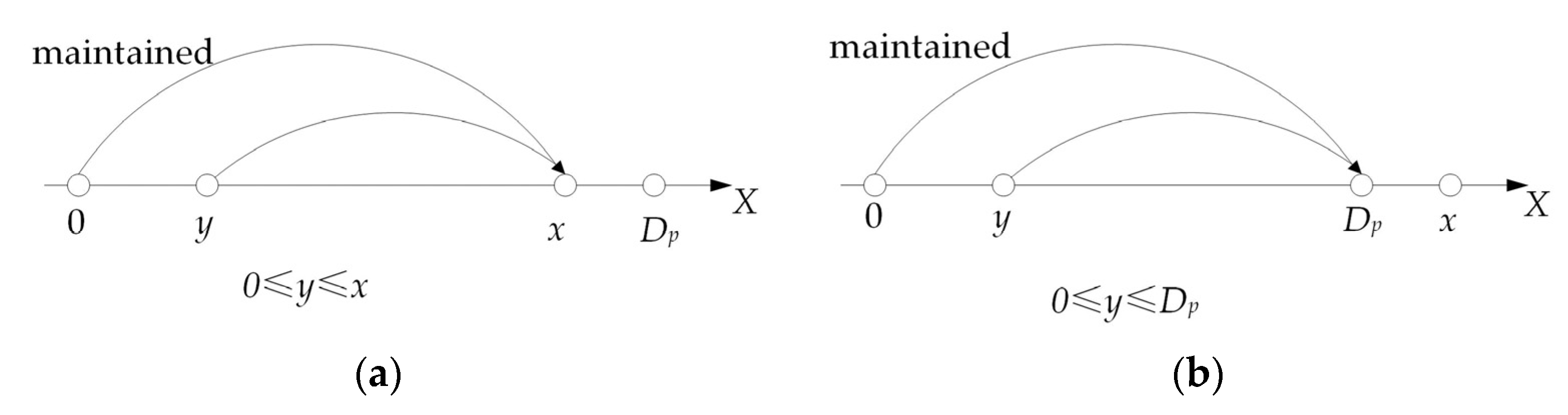
Figure 2.
Schematic of three situations. (a) When detected, if the equipment state satisfies 0 < x(tn) ≤ Dp, the maintenance is not needed, and there is no shortage. (b) When detected, if the equipment state satisfies Dp < x(tn) ≤ Df, preventive maintenance is needed. If the PM time is longer than the inventory consumption time, there is a shortage. (c) When detected, if the equipment state satisfies x(tn) > Df, corrective maintenance is needed. If the corrective maintenance time is longer than the inventory consumption time, there is a shortage.

Figure 3.
Iteration diagrams. (a) The genetic algorithm with an elite strategy is used. (b) The improved genetic algorithm with an elite strategy is used.
Figure 3.
Iteration diagrams. (a) The genetic algorithm with an elite strategy is used. (b) The improved genetic algorithm with an elite strategy is used.
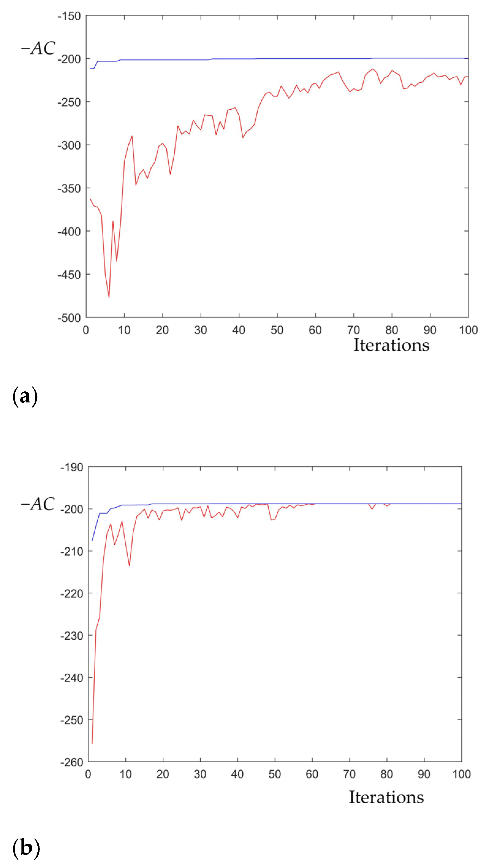
Figure 4.
Three-dimensional scatter plots. (a) Integrated three-dimensional scatter plot shows the overall trend of the solution. (b) Partial three-dimensional scatter plot shows the local trend of the solution more clearly.
Figure 4.
Three-dimensional scatter plots. (a) Integrated three-dimensional scatter plot shows the overall trend of the solution. (b) Partial three-dimensional scatter plot shows the local trend of the solution more clearly.
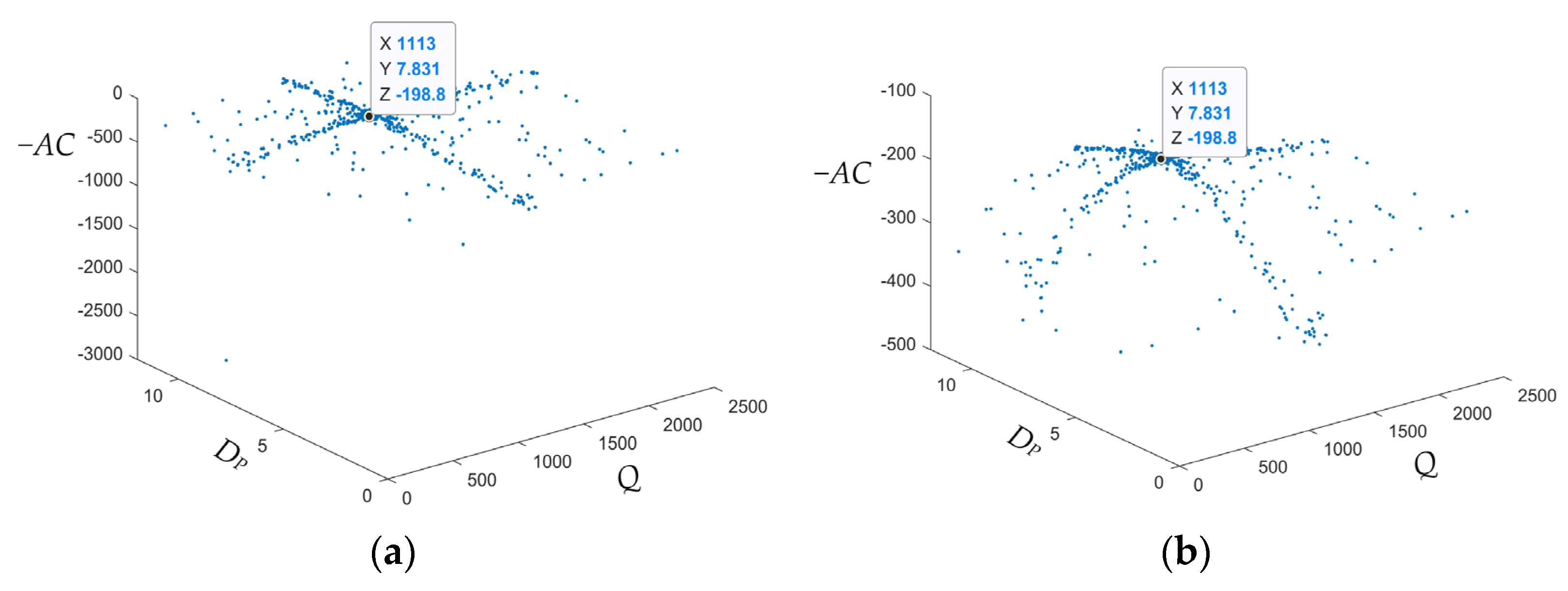
Figure 5.
Influence of parameters on the optimal quantity Q*.
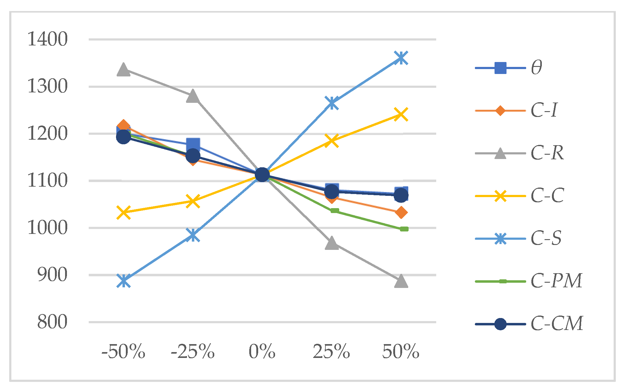
Figure 6.
Influence of parameters on the PM threshold Dp*.

Figure 7.
Influence of parameters on the average cost rate AC*.


Table 1.
Parameter value table.
| Parameters | Description |
|---|---|
| Q | economic production quantity, decision variable |
| Dp | preventive maintenance threshold, decision variable |
| Df | equipment failure threshold |
| pr | the production rate of the system |
| dr | the demand rate of the system |
| θ | fixed low-quality product ratio in qualified products |
| CI | unit product inventory cost |
| CR | unit unqualified product repair cost |
| CS | unit product shortage cost |
| CC | detection cost each time |
| CPM | preventive maintenance cost each time |
| CCM | corrective maintenance cost each time |
| x(t) | state of the equipment at time t |
| s(x) | the steady-state probability density function of equipment state x |
| g1(tpm) | probability density function of preventive maintenance time tpm |
| g2(tcm) | probability density function of corrective maintenance time tcm |
Table 2.
Input parameters.
| Parameter | Value | Parameter | Value |
|---|---|---|---|
| pr (unit/day) | 200 | Df | 12 |
| dmax (unit/day) | 160 | CI (Yuan/unit/day) | 0.5 |
| θ | 0.1 | CR (Yuan/unit) | 10 |
| p0 | 0.004 | CS (Yuan/unit) | 20 |
| η | 0.071 | CC (Yuan/Each time) | 150 |
| α | 0.0046 | CPM (Yuan/Each time) | 1800 |
| β | 1.26 | CCM (Yuan/Each time) | 4500 |
| μ | 0.1 |
Table 3.
Sensitivity analysis results.
| Parameter | Variation | The Optimal Quantity Q* | The Optimal PM Threshold Dp* | The Average Cost Rate AC* |
|---|---|---|---|---|
| - | Basic case | 1113 | 7.831 | 198.7637 |
| θ | −50% | 1201 | 7.6735 | 207.8333 |
| −25% | 1177 | 7.7005 | 203.2433 | |
| 25% | 1081 | 7.9021 | 194.477 | |
| 50% | 1073 | 7.9547 | 190.3974 | |
| CI | −50% | 1217 | 7.5325 | 191.6533 |
| −25% | 1145 | 7.7108 | 195.3027 | |
| 25% | 1065 | 7.9359 | 202.1052 | |
| 50% | 1033 | 8.048 | 205.3371 | |
| CR | −50% | 1337 | 7.215 | 181.8428 |
| −25% | 1281 | 7.5831 | 191.0104 | |
| 25% | 969 | 8.1578 | 206.1737 | |
| 50% | 888 | 8.6392 | 212.4117 | |
| CC | −50% | 1033 | 8.0755 | 188.186 |
| −25% | 1057 | 7.9303 | 193.5904 | |
| 25% | 1185 | 7.6226 | 203.6904 | |
| 50% | 1241 | 7.4475 | 208.3536 | |
| CS | −50% | 888 | 8.2554 | 183.1767 |
| −25% | 985 | 8.0255 | 192.0107 | |
| 25% | 1265 | 7.5141 | 204.1839 | |
| 50% | 1361 | 7.316 | 208.5963 | |
| CPM | −50% | 1201 | 6.367 | 153.026 |
| −25% | 1153 | 7.2189 | 176.8459 | |
| 25% | 1037 | 8.365 | 220.6385 | |
| 50% | 998 | 9.2227 | 235.0724 | |
| CCM | −50% | 1193 | 9.9544 | 167.593 |
| −25% | 1153 | 8.5109 | 189.6088 | |
| 25% | 1077 | 7.2975 | 206.448 | |
| 50% | 1069 | 6.9545 | 210.8357 |
Publisher’s Note: MDPI stays neutral with regard to jurisdictional claims in published maps and institutional affiliations. |
© 2022 by the authors. Licensee MDPI, Basel, Switzerland. This article is an open access article distributed under the terms and conditions of the Creative Commons Attribution (CC BY) license (https://creativecommons.org/licenses/by/4.0/).
Share and Cite
MDPI and ACS Style
Gao, Z.; Wang, H.; Zhang, H. The Decision of Production Systems with Quality-Contingent Demand and Condition-Based Maintenance. Systems 2022, 10, 20. https://doi.org/10.3390/systems10010020
AMA Style
Gao Z, Wang H, Zhang H. The Decision of Production Systems with Quality-Contingent Demand and Condition-Based Maintenance. Systems. 2022; 10(1):20. https://doi.org/10.3390/systems10010020
Chicago/Turabian StyleGao, Zhenhua, Hongjun Wang, and Hongliang Zhang. 2022. "The Decision of Production Systems with Quality-Contingent Demand and Condition-Based Maintenance" Systems 10, no. 1: 20. https://doi.org/10.3390/systems10010020
Note that from the first issue of 2016, this journal uses article numbers instead of page numbers. See further details here.