
Behavioral Framework of Asset Price Bubbles: Theoretical and Empirical Analyses

1
School of Finance and Economics, Jiangsu University, Zhenjiang 212013, China
2
Economics and Management School, Wuhan University, Wuhan 430072, China
*
Author to whom correspondence should be addressed.
Systems 2022, 10(6), 251; https://doi.org/10.3390/systems10060251
Submission received: 10 November 2022
/
Revised: 3 December 2022
/
Accepted: 7 December 2022
/
Published: 9 December 2022
(This article belongs to the Section Complex Systems)
Abstract
:Sentiment and extrapolation are ubiquitous in the financial market, and they are not only the embodiment of human nature, but also the primary drivers of asset price bubbles. In this study, we first constructed a theoretical model that included fundamental traders and extrapolated investors, and we assessed the time series characteristics of asset prices under different types of information shocks. According to the research results, good news about the fundamentals can lead to positive asset price bubbles, and correspondingly, bad news can lead to negative asset price bubbles; however, the decrease in asset prices in the case of negative bubbles is not as substantial as the increase in prices in the case of positive bubbles, and the time for prices to reverse is also long, which can be explained by the short-selling constraints. According to the comparative static analysis, the scales of the positive and negative foams depend on the proportion of investors in the market and the extrapolation coefficient. We verified the conclusion of the theoretical model from two aspects: (1) we analyzed the relationship between investor sentiment and the prevalence of informed trading, and according to the results, the increase (decrease) in investor sentiment can reduce the information content of asset prices and increase price volatility; however, the impact of low sentiment is not substantial, which preliminarily tests the conclusion of the theoretical model; (2) we examined the relationship between the cumulative change in investor sentiment and future portfolio returns, and we found that the cumulative increase in investor sentiment can have a positive impact on future portfolio returns at the initial stage, and depress future portfolio returns in the long term, which forms positive asset price bubbles. The cumulative depression of investor sentiment can depress the future portfolio returns at the initial stage, and positively influence the future portfolio returns in the long term, which forms negative asset price bubbles. Moreover, these two nonlinear relationships exhibit cross-sectional differences in different types of asset portfolios, which further validates the key proposition of the theoretical model.
1. Introduction
Under the traditional finance framework, investors are considered to be absolutely rational agents. At the belief level, they update their expectations based on the Bayesian law. At the preference level, they use the expected utility theory to make investment decisions. However, these traditional rational assumptions cannot explain various anomalies in the market. In order to make the theory closer to reality, behavioral finance theory uses psychology and the arbitrage limit theory as the two cornerstones [1] to modify the asset pricing model. At the belief level, a large number of expectation-updating processes that violate the Bayesian rule are depicted. The important assumption about investor expectation is expectation extrapolation, that is, investors’ estimates of the future value of certain variables are positively correlated with the historical value of the variable [2].
Barberis [2] suggests that behavioral finance focuses on three theoretical frameworks: extrapolation expectation theory, overconfidence theory, and prospect theory represented by loss aversion. Among them, the first two are belief-based theoretical models, and the latter is a preference-based theoretical model. In addition, the extrapolation expectation model implicitly contains the opinion divergence model based on overconfidence, which is the root cause of excess trading volume. Therefore, as a representative of the behavioral financial model based on belief, the extrapolation expectation model is of great significance in explaining market anomalies.
According to the dividend discount model, the stock price is equal to the discount value of future cash flows. However, many studies have shown that price changes in financial markets are difficult to explain through the changes in investors’ rational expectations of future cash flows or discount rates [3,4]. In other words, the change of investors’ rational expectations is not the main reason for the excessive volatility of asset prices, and the volatility puzzle cannot be explained through the traditional rational framework. Moreover, the historical data of the US market shows that the price dividend ratio exhibits stability in the time series, and a higher price dividend ratio is accompanied by a moderate price dividend ratio. The reduction in price dividend ratio can be achieved through two paths: the increase in dividend payment or the decrease in price. Campbell and Shiller [5] find that a higher price dividend ratio does not necessarily result in a higher dividend growth rate. Therefore, the higher price dividend ratio in the previous period usually leads to the decline of future prices (yield decline). Therefore, the change of the above price dividend ratio can only predict the future price, which is the mystery of the predictability of the price dividend ratio at the time series level. The price dividend ratio is not only an indicator to verify the mystery of predictability, but also a core variable to discuss the volatility puzzle. Therefore, many studies believe that the predictability in time series and excessive price volatility reflect the same phenomenon [2], and that extrapolation expectations play an important role in explaining the anomalies in the aggregate market.
The extreme case of excessive volatility in the aggregate market is the formation and bursting of bubbles. Since the bubbles can simultaneously include the excessive volatility of asset prices, short-term momentum, long-term reversal, and the mystery of predictability, the discussion of this extreme anomaly has strong theoretical significance and can significantly promote the development of behavioral finance. Although Cutler et al. [6], De Long et al. [7], Hong and Stein [8], Barberis and Shleifer [9], and Barberis et al. [10] discuss excessive volatility and the mystery of predictability by building an extrapolated expectation model, they do not discuss bubbles. Barberis et al. [11] and Liao et al. [12] construct a theoretical framework to discuss the relationship between extrapolation expectations and bubbles but are unable to characterize negative bubbles under bearish news due to the short-selling constraints faced by each type of investors.
As for the economic mechanism behind the bubbles, Xiong and Yu [13] provide a series of theories to explain it. Among the eight causes of bubbles contained in this set of theories, there are five mechanisms related to extrapolation expectations, namely gambling behavior, resale option behavior, rational non consensus, feedback loop theory, and riding the bubble. Hence, we took the extrapolation belief as the theoretical basis of the feedback mechanism, built a theoretical model that included fundamental traders and extrapolation investors, assessed the characteristics of asset price changes upon the initial receipt of good and bad news, conducted a comparative static analysis around the scale of the bubbles, and studied the micro-mechanisms of the bubbles from the theoretical level. Investor confidence, expectation, or risk aversion, although expressed differently, fall into the category of investor sentiment [14], and we can unify the above conclusions as the “two-way feedback between sentiment and historical prices”, and then conduct an empirical test from the perspective of the investor sentiment index. First, we investigated the relationship between investor sentiment and the proportion of informed trading in an attempt to prove that increasing (decreasing) investor sentiment can reduce the information content of asset prices and increase their volatility. However, asset mispricing mainly occurs in periods of increasing sentiment, and not in periods of decreasing sentiment, which preliminarily confirms the rationality of the theoretical model’s conclusions. Second, in view of the two-way feedback between investor sentiment and historical price changes, the sustained increase (decrease) in sentiment can be regarded as the origin of the bubbles; thus, the existing sentiment index also needs to be expanded to reflect the existence of sentiment feedback. In this study, we examined the relationship between the cumulative-type investor sentiment index and future portfolio returns, and we comprehensively tested the conclusions of the theoretical model from the aggregate level to the cross-sectional level.
Compared with the existing research, the contribution of this paper lies in the following: (1) Contrary to Barberis et al. [11], we considered the interaction between pure “noise traders” and pure “fundamental traders”, which reduced the complexity of the theoretical modeling and analysis to a certain extent. More importantly, although we greatly reduced the complexity of the model by modifying Barberis et al. [11]’s theoretical model setting, it is mainly for the purpose of depicting negative bubbles, and the ultimate purpose of the simple model is to highlight the core mechanism proposed in this paper—the advantage of expectation extrapolation in identifying the formation and collapse of bubbles, further reflecting the important role of this belief bias in the field of behavioral finance. (2) In the existing feedback trading models, we assessed the bubble scenario under the impact of positive information; however, the impacts of investor sentiment on asset prices under different types of information shocks are asymmetric. What conclusions can we draw from the negative information impact? In this study, we removed the short-selling constraint hypothesis of Barberis et al. [11], attempted to assess the negative bubble scenario under the impact of negative information, and compared positive and negative bubbles, thereby enriching the behavioral financial theory and deepening our understanding of the financial market. (3) According to Barberis et al. [11], although fundamental traders in the market exist, the reason that extrapolated investors can still generate bubbles is that short-selling constraints have forced fundamental traders to leave the market in the face of overvalued asset prices. However, as a rational agent with risk aversion characteristics, does the reason for not arbitraging have nothing to do with price risk? This is evidently not in line with reality. Hence, under the condition of removing the assumption of the short-selling constraint, we tried to analyze the role of fundamental traders in the scenario of bubble formation from the perspective of risk compensation with the aim of promoting behavioral finance research. (4) The prevailing investor sentiment index has proven to be a contrarian indicator of future asset returns [14,15], which confirms that investor sentiment can affect asset returns in the short term, but this only increases the volatility of the asset prices, and it is not enough for us to explain the existence of bubbles because bubbles are only a subset of the abnormal volatility of asset prices. In this study, we expanded the BW sentiment index based on Berger and Turtle [16] to make it echo the sentiment feedback theory at the empirical level, which not only enriches the investor sentiment theory, but also broadens the interpretation scope of the sentiment index. The conclusions of this paper have certain practical value in the identification of asset price bubbles, the formulation of investment strategies, and the supervision of abnormal fluctuations in stock prices [17].
2. Model
2.1. Basic Assumptions
Based on Barberis et al. [11], Liao et al. [12], and Mendel and Shleifer [18], we consider a economy in which there are two types of assets: risk-free assets and risky assets. The supply of risky assets is equal to , which is liquidated in , and the risky dividend paid is .
where
The value of is public information in time 0, and is the information shock in t. The supply of risk-free assets is fully elastic, and the yield is 0. Next, we will gradually complete the construction of the basic model through a series of assumptions.
Assumption 1:
The market includes two types of investors: extrapolated investors and fundamental traders, and their market proportions are and, respectively ().
Assumption 2:
Fundamental traders have the characteristics of bounded rationality, and their investment decisions follow the CARA utility optimization criteria.
We take the assumption of “bounded rationality” here from Barberis [2]: fundamental traders cannot understand the demand formation process of other participants in the market but simply assume that, in the future, the share of the risk assets held by other participants in the total share of risk assets is equivalent to the proportion of the number of participants in the total number of market participants.
The decision made by fundamental traders in a period () is to maximize the CARA utility function by holding the optimal number of risky assets. The CARA utility function is as follows:
Lemma 1:
With the CARA utility function in the form of , the expected utility optimization problem is equivalent to the maximization of the following functions under the conditions of and (Please see Appendix A):
The demand function of fundamental traders is as follows:
For (4), the numerator is the expected price of the risk assets at . Therefore, the numerator represents the expected price change in the next period (See the Appendix A for the derivation of this formula).
If there are only fundamental traders in the market, then we can obtain it through market clearing, such as :
Due to the fact that (5) is the market-clearing price that is completely determined by fundamental traders, which can be regarded as the “fundamental value of risky assets”, we set it as :
Assumption 3:
Extrapolated investors are irrational agents, and their demands exhibit a linear relationship with the extrapolation belief.
It is worth noting that, different from Mendel and Shleifer [18], the irrational investors in this paper do not intuitively generate misconceptions about fundamental information, but rather describe the noise trading agent by extrapolating the historical information. This idea originates from Barberis et al. [11], but the difference is that we are talking about purely irrational agents and will not be affected by the short-selling constraint. For fundamental traders, the form of demand function is generally the same as that in the above references. The reason that these two different types of agents derived from the optimization of the CARA utility function is that we still refer to Mendel and Shleifer [18]’s method to facilitate the mathematical derivation.
Consistent with Hu Changsheng et al. [19], the sentiment system of irrational investors is composed of “feedback”, which is affected by early prices. However, the sentiment system constructed in the existing literature is not sufficient because extrapolated investors do not solely make decisions based on recent price changes; longer-term price fluctuations are also within their decision-making scope. Therefore, we define the demand function of the extrapolated investors as follows (See the Appendix A for the derivation of this formula):
2.2. Market Equilibrium
We can obtain the following asset equilibrium prices through the market-clearing conditions :
In (8), the first item indicates the expected value of the asset price anchored to the final cash flow. The second item indicates that, when the historical price shows a strong increase, the extrapolated investors will show more optimistic expectations for future price changes, thus increasing the demand for risky assets and further driving up the price. The third item indicates the risk discount, which compensates the investors who bear risks [20].
3. Parameter Settings of Numerical Simulation
In order to discuss the formation and collapse of asset price bubbles, it is necessary to determine the assignment of the relevant parameters. The parameters related to risky assets are , , , and . The parameters related to investors are , , , and .
determines the weight given to recent price changes when extrapolated investors predict future price changes, which thus affects the trading intensity. Based on the survey data of Greenwood et al. [21], Barberis et al. [11] set . Due to the fact that irrational investors in the Chinese market pay more attention to short-term price fluctuations, we set .
Let us assume that , . We can see that 70% of the market participants are retail investors, which is consistent with the situation of the Chinese market.
We set the other parameters as follows: initial expected dividend: ; standard deviation of cash-flow shocks: ; supply of risky asset: ; risk aversion coefficient: ; number of periods: .
4. Numerical Simulation under Impact of Good News
4.1. Asset Price Characteristics in Bubbles
In Manias, Panics, and Crashes: A History of Financial Crises, the author succinctly depicts the basic characteristics of asset price foam, which is bubbles that are caused by strong and favorable cash-flow information. Based on the above parameters, we set the cash-flow sequence as: , and we conducted the numerical simulation through Equations (7) and (9).
According to Figure 1, the solid line is the asset price, and the dotted line is the fundamental value. At , the strong information shock in the market pushes up the asset price. At , the extrapolated investors observe the stronger increase in the price at and become more optimistic about the future changes in risky assets, which further pushes up the price. The continuous increase in the price maintains a high level of extrapolated investor sentiment. At , the more optimistic extrapolated investors push the price to a higher level. However, asset prices begin to fall at . So far, the maximum price increase at has shown a decreasing trend, and according to (7), the impact of the early positive information shocks on the extrapolated investors gradually weakens over time, which prompts the extrapolated investor sentiment to turn from optimism to pessimism and causes the price to drop through the selling of assets.
What role do fundamental traders play during the above mentioned period? According to Loewenstein and Willard [22], the consumption risk generated by noise traders should be categorized as fundamental risk. As rational agents, the risk aversion characteristics of fundamental traders mean that, if they want to arbitrage against mispricing, then they must ensure that the fundamental values contain risk discounts or premiums as compensation for the risks faced by arbitrage trading. Consequently, fundamental traders must wait until the extrapolation traders push the price to a high point before selling at this price level, which can not only obtain considerable returns but can also lead to the bursting of bubbles.
The theoretical framework under the impact of good news successfully depicts the bubbles. Specifically, we can divide the bubbles into the combination of short-term and medium-term momentum effects and long-term reversal effects [19]. The further increase in the price at caused by the increase in the price at can depict the momentum effect: the increase in the price at makes the extrapolated investors more optimistic at , which further drives up the price. Additionally, the continuous increase in the prices in the period leads to the continuous decrease in the prices in the period , which depicts the long-term reversal effect. The active buying of extrapolated investors, which leads to the overpricing of assets, reflects that the assets have performed well for long periods in the past. A high valuation must be accompanied by a low return. The continuous increase in prices in the period and the continuous decrease in prices in the period describe the basic characteristics of bubbles.
4.2. Comparative Static Analysis
According to (9), the equilibrium price of assets is related to the market proportion of the investors (, ) and the reaction intensity of the extrapolated investors (), regardless of whether the scale of the bubbles is also related to these factors, which prompted us to carry out the following comparative static analysis. In this paper, we discuss the influencing factors of bubbles based on different fundamental trader proportions () and extrapolation coefficients ().
According to Figure 2, as the proportion of fundamental traders in the market increases (), they play a stronger role in repairing the volatility of the asset prices, pushing them back to their fundamental values, and reducing the sizes of the bubbles, which is consistent with the conclusions of De Long et al. [7], Hu Changsheng et al. [19], and Chen Cong et al. [22]. Then, with the increase in the extrapolation coefficient for the extrapolated investors (), the asset prices are closer to fundamental values, and the scale of the bubbles is smaller. To understand this conclusion, we first reviewed (7):
Let both sides of (11) multiply , and subtract (8) to obtain:
The first term of (11) shows that bubbles have a natural tightening property. As time goes by, the price changes that once caused the extrapolated investor sentiment to increase become a thing of the past, which weakens it. The key that can make the recent price changes have a significant effect is : if is larger, then the extrapolated investors will pay more attention to the recent price changes. As time goes on, the impact of the historical price changes on the sentiment of the extrapolated investors will be weaker, which makes it difficult to maintain the continuous price increase.
The following is a summary of the above analysis:
Proposition 1:
In the scenario of initial positive information shock, the asset price increase causes extrapolated investors to become more optimistic about future asset price changes, which creates a further price increase and higher extrapolation belief. With the passing of positive information shocks, the impact of the historical price increases on the expectations of the extrapolated investors gradually weakens, which leads to the gradual depression of the extrapolated investor sentiment and the selling of assets, which explains the formation and collapse of asset price bubbles. The scale of the bubbles is related to the market proportion of the investors and the extrapolation coefficient: when the proportion of fundamental traders increases, the extrapolation coefficient increases, and the scale of the bubbles decreases.
5. Numerical Simulation under Impact of Bad News
5.1. Asset Price Characteristics in Bubbles
To fill the gap in the existing literature, and to examine whether there are differences in the impacts of different types of information on investor sentiment and asset prices, we discuss the impact of bad news shocks on bubbles. While keeping the other parameter settings in Table 1 unchanged, we considered the following cash-flow shock sequence: , and we conduct a numerical simulation through (6) and (8).
According to Figure 3, with the introduction of negative information about the fundamentals into the market, asset prices fall, which leads extrapolated investors to exhibit pessimistic expectations about future price changes, prompting them to further sell their assets, which drives the prices down. The continuous decrease in the prices forms negative bubbles. With the passing of the bad news and the extension of the time interval, the influence of the bad news gradually passes and the extrapolated investors resume their optimistic expectations regarding future prices. The prices begin to rebound with the active buying of the extrapolated investors.
In general, Schiller’s feedback theory is also applicable to bad news [23]; however, we can still observe some differences relative to the case of positive information. For example, under the impact of good news, the asset price rose from 90 to 98, but the price under the impact of negative information only fell from 78 to about 74, which indicates that the response of the asset prices to positive and negative news shocks is asymmetric because, even without short-selling restrictions, selling in the financial market is still more difficult than buying [24]. As examples of irrational investors, individual investors have narrow investment channels and are more vulnerable to short-selling constraints [25]. In addition, as the reverse trading object of extrapolated investors, fundamental traders are not restricted when the asset pricing is too low. By buying the asset at a low price and correcting the price error in time, the price starts to rebound at . However, under the impact of positive information, because fundamental traders are unwilling to carry out reverse arbitrage with extrapolated investors with high sentiment, the rational agent is affected by the short-selling constraint at this time, which results in the price rebounding at around .
Similarly, in the face of price decline, extrapolated investors believe that prices will further decline in the future, and they thus sell large numbers of assets. To encourage fundamental traders to buy assets when prices are undervalued, the fundamental values must include risk discounts. However, due to the limited number of assets sold by extrapolated investors, the asset price does not contain much noise. This low risk also makes the risk-discount component in the price less than the above-risk premium component.
5.2. Comparative Static Analysis
The negative bubbles under the impact of negative information are also related to the proportion of investors and the extrapolation coefficient. According to Figure 4, as the proportion of fundamental traders increases (), their ability to correct the undervaluation is enhanced, and the size of the bubble accordingly shrinks. If the extrapolation coefficient of the extrapolated investor is larger (), then it is easier to eliminate the impact of the historical price changes, more difficult for prices to continuously fall, and the scale of the bubbles also becomes smaller.
The following is a summary of the above analysis:
Proposition 2:
In the scenario of negative information shock, the decrease in the asset prices leads to pessimistic extrapolated investor expectations about future price changes, and they then sell their assets, which leads to further price decreases. With the passage of time, the impact of the historical price changes on the extrapolated investors gradually weakens, and the extrapolated investors finally resume their optimistic expectations regarding future price changes and buy assets to promote the price rebound and form negative bubbles. However, regardless of the degree of the price decline and reversal cycle, the scale of the negative bubbles is smaller than that of positive bubbles, which indicates that selling is more difficult than buying in the financial market. The scale of the negative bubbles, which takes the underpricing of asset prices as its manifestation, is still inversely related to the proportion of fundamental traders and the extrapolation coefficient.
6. Empirical Test of Investor Sentiment and Ratio of Informed Trading
The key conclusion of the above model is that the high (low) investor sentiment under the impact of positive (negative) information leads to the serious deviation in the asset prices from the fundamental values, which forms positive (negative) bubbles. The scale of the bubbles is closely related to the proportion of fundamental traders and the extrapolation coefficient of the extrapolated investors. Hu Changsheng et al. [15] argue that we can judge the investor structure of the market by the level of the investor sentiment. We assessed the relationship between investor sentiment and the proportion of informed trading, and we preliminarily tested the core proposition generated by the theoretical analysis.
6.1. Data Description and Variable Construction
The variables involved in this section are as follows: investor sentiment index; unemployment rate; illiquidity index; market volatility; daily return rate of individual shares; trading volume; net profit and owner’s equity of listed companies; quarterly GDP growth rate. We took all the sample data from the CSMAR database, and the sample range is from February 2003 to December 2021.
6.1.1. Investor Sentiment Index
The construction method of the investor sentiment index originated from Baker and Wurgler [14]. However, the sentiment index still contains some information about economic fundamentals, which needs further purification to measure the investor behavioral bias [26]. Therefore, we regressed the BW investor sentiment index with the Amihud illiquidity index, unemployment rate, and market volatility, and we took the resulting residual as the final investor sentiment index.
6.1.2. Control Variable
We use the real GDP growth rate and ROE synchronization to control the impact of the macroeconomic factors. Different from the US market, China’s ROE data are only taken at an annual frequency. In order to reduce them to a quarterly frequency, we expressed the ROE as the sum of the net profits/owner’s equity. Subsequently, in each quarter, we regarded the ROE of the individual shares as the predicted variable, and the market- and industry-level ROEs as the explanatory variables, and we conducted rolling regression between the individual-stock ROE and market and industry ROEs over the 12 previous quarters. Among them, we divided the listed companies into five sectors, according to the practice of the CSMAR database: public utilities; real estate; comprehensive; industrial; commercial. Based on this, we calculated the market and industry ROEs for each quarter by the method of value weighting.
and are the linear time trend variables. The former is constructed by taking 1 in the first month of the sample interval and moving it according to the marginal change in the 1. The latter is the square term of the former. We used these two control variables to control the long-term trend of the idiosyncratic return volatility [27] and its reversal [28].
6.1.3. Informed Trading Variable
The construction of the informed trading variable () originated from Llorente et al. [29], and the specific implication is as follows: the change in the trading volume supported by information is usually accompanied by momentum, and volume changes that are not supported by information are usually accompanied by reversals. We can obtain the according to the following model:
where is the return of the stock () on a day (); is the logarithmic trading volume of the stock () on a day () (in order to eliminate the impact of this trend, we subtracted the average trading volume over the previous 200 trading days from the trading volume of each day); is the random disturbance term; is the core coefficient, which can capture the .
We estimated the for each month based on (12). If , then the daily abnormal trading volume of the stocks within one month is related to the momentum of the returns, indicating the prevalence of informed trading; otherwise, it is negative. For the convenience of narration, we multiplied by 100. Then, we calculated the arithmetic mean value of the individual stock () each month, and we expanded it to the aggregate market level. According to Table 2, the monthly at the aggregate market level showed relatively stable change (17.203).
6.2. Empirical Analysis
To explore the relationship between investor sentiment and informed trading, we constructed the following empirical model:
where the core variables are and , as they capture the asymmetric impact of the investor sentiment on the proportion of informed trading. When the investor sentiment is greater than 0, the is equivalent to the sentiment index itself; otherwise, it is 0. If the investor sentiment is less than 0, then the is the absolute value of its sentiment index; otherwise, it is 0.
According to the empirical results in Table 3, the sign of is negative and significant at the level of 5%, which indicates that the intensity of the informed trading will weaken during the period of high investor sentiment, which confirms the impact of extrapolated investors on asset prices under the impact of positive information. Although low investor sentiment can also reduce the intensity of the informed trading (the sign of is negative), it does not exhibit significance because, in the face of the price decline caused by bad news, pessimistic extrapolated investors cannot substantially and continuously make the price deviate from the fundamental value, which results in a weak price decline that soon rebounds. In addition, with the decline in the proportion of fundamental traders and the reduction in the extrapolation coefficient, the market enters a period of high investor sentiment that is dominated by extrapolated investors. The decrease in the intensity of informed trading also supports the conclusion of the comparative static analysis.
Thus far, we have preliminarily confirmed Propositions 1 and 2 of the theoretical model.
7. Investor Sentiment Accumulation and Asset Return
Shiller [23] suggests that historical price increases stimulate investor confidence and their expectations further increase, which further pushes up the prices, and the investor confidence and expectations simultaneously become more extreme. This historical-price-driven belief deviates from the rational paradigm and can be included in the investor sentiment category [14]. Although we can use the BW sentiment index to effectively measure the investor belief bias and affect asset returns, this sentiment index cannot reflect the two-way feedback mechanism between sentiment and historical prices. To further test the conclusions of the theoretical model, we expanded the BW sentiment index to discuss the relationship between the cumulative increase (decrease) in investor sentiment and future portfolio returns from the aggregate to the cross-sectional level. However, a complete bubble scenario should include the continuous increase in asset prices and the deviation from fundamental values, which are eventually accompanied by a more drastic decline. There may not be a linear relationship between the cumulative change in sentiment and future asset returns, which leads us to a discussion of the logic between these two variables.
7.1. Data Description and Variable Construction
The variables involved in this section are as follows: investor sentiment change index; investor sentiment cumulative index; daily stock return; monthly stock return; risk-free interest rate; monthly stock market return; monthly circulating stock market value; stock volatility; Amihud illiquidity index. In order to ensure the accuracy and continuity of the sample stock data, we removed the ST shares, financial shares, and real estate shares from all the A-shares and obtained 4620 sample stocks. We took all the sample data from the CSMAR database, and the sample coverage range is from February 2003 to December 2021.
7.1.1. Investor Sentiment Cumulative Index
The investor sentiment cumulative index is the core explanatory variable in this section. Following Baker and Wurgler [30] and Berger and Turtle [16], we construct the investor sentiment change index () and expanded it as follows: First, we defined the investor sentiment cumulative high index as , which indicates the continuous increase in investor sentiment as of . Starting from the first month of the sample interval, we set . For each subsequent month, we accumulated the series in which was consecutively greater than 0. Once the investor sentiment decreased () in a certain month, we set again. So far, we can extract the part of investor sentiment that continues to increase, which lays the foundation for depicting the bubbles under the impact of positive information. Second, we defined the investor sentiment cumulative low index as , which indicates the continuous decrease in the investor sentiment as of . At the starting point of the sample interval, we set . Then, we accumulated the numerical sequences with consecutive . Once in a certain month, we set again. We extracted the part of the investor sentiment that continued to decline, which was helpful for us to depict the negative bubbles caused by negative information shocks. We made a small change by calculating the absolute value of the part of the investor sentiment that continuously changed to negative.
7.1.2. Portfolio Variable
To conduct an empirical analysis from the aggregate level to the cross-sectional level, it is necessary to determine the dependent variables. At the aggregate level, we introduced the market equal-weighted return rate and value-weighted return rate. The weighted average return rate of the circulating market value and equally weighted average of all the stocks in the whole market and within the calculation scope are all the A-shares. At the cross-sectional level, we divided the sample stocks in each month into 10 groups according to the circulating market value, liquidity, and volatility at the end of the previous month, and we calculated the equal-weighted return rate of each portfolio using the monthly frequency return rate of the individual stocks. Then, we generated descriptive statistics on the core variables in this section. To save space, we only present the extreme asset portfolio generated by the cross-section grouping.
According to Table 4, the mean and standard deviation of the equal-weighted market return rate were 1.416 and 9.477, respectively, which were higher than the 0.861 and 7.959, respectively, of the value-weighted market return rate. This is because the equal-weighted market portfolio assigns a higher weight to small-cap stocks, which results in relatively sharp fluctuations, which indicates that, when we use the value-weighted portfolio return rate rather than the equal-weighted portfolio return rate, the extent of some of the anomalies in the market will be reduced or will even disappear [15]. For other asset portfolios, small-cap stocks, low-liquidity stocks, and high-volatility stocks also show higher means and standard deviations, which is due to the speculative characteristics of individual investors. Their trading behavior is more vulnerable to gambling preferences, investment entertainment, and other factors, and the investors are keen to make investments that “obtain high returns with minimal probability and bear small losses with maximum probability” [31], which fully conforms to the characteristics of stocks with low market value, low liquidity, and high volatility. As individual investors hold these high-risk portfolios, they naturally generate higher average returns for them.
7.2. Empirical Analysis
7.2.1. Cumulative High Investor Sentiment and Asset Returns
We tested the bubbles under the impact of positive information through the following empirical model:
where is the return rate of the portfolio () in a period (); is the risk-free rate in a period (); is the sentiment cumulative growth index; is the random error term. We will discuss the relationship between the different portfolio returns and sentiment cumulative growth indices.
We first observe the empirical results at the aggregate level in Table 5. The of the equal-weighted and value-weighted market portfolios is positive and significant at the 5% level, which indicates that the cumulative growth of sentiment will have a significant positive impact on the future market returns at the initial stage, which causes the continuous price increase. The is negative and has significance at the level of 10%, which indicates that the cumulative growth of sentiment will have a significant negative impact on the future market returns in the long term, which prompts the prices to fall. Therefore, the cumulative growth of sentiment can depict the formation and bursting of bubbles at the aggregate level. In the case of the equal-weighted market portfolio, the absolute values of and are both greater than those in the value-weighted market portfolio (3.372 > 2.612 vs. 0.520 > 0.438, respectively), which indicates that the equal-weighted market portfolio is more vulnerable to sentiment shock, which makes the degree of the anomalies more obvious, which results in a larger bubble. Therefore, we chose the equal-weighted portfolio as the research object in this section.
At the cross-sectional level, and result from the grouping of the size, liquidity, and volatility, which also have significantly positive and negative performances, which indicates that the cumulative growth of sentiment can also have a significant nonlinear impact on portfolio returns with different characteristics, which forms a bubble. In addition, for small-cap stocks, low-liquidity stocks, and high-volatility stocks, which individual investors tend to hold on to, the absolute values of and are also greater than those of large-cap stocks, high-liquidity stocks, and low-volatility stocks, which also confirms that there is a cross-sectional difference in the impact of the sentiment cumulative growth on portfolio returns. On the whole, although the symbol of is consistent with the expectations and has significance, its absolute value and t-statistics are far less than those of , which indicates that the bubble generated in the market is not easy to burst, which reflects the weak strength of China’s fundamental traders, whose reverse arbitrages have failed to timely and effectively correct the price overvaluation and rapidly return prices to their fundamental values.
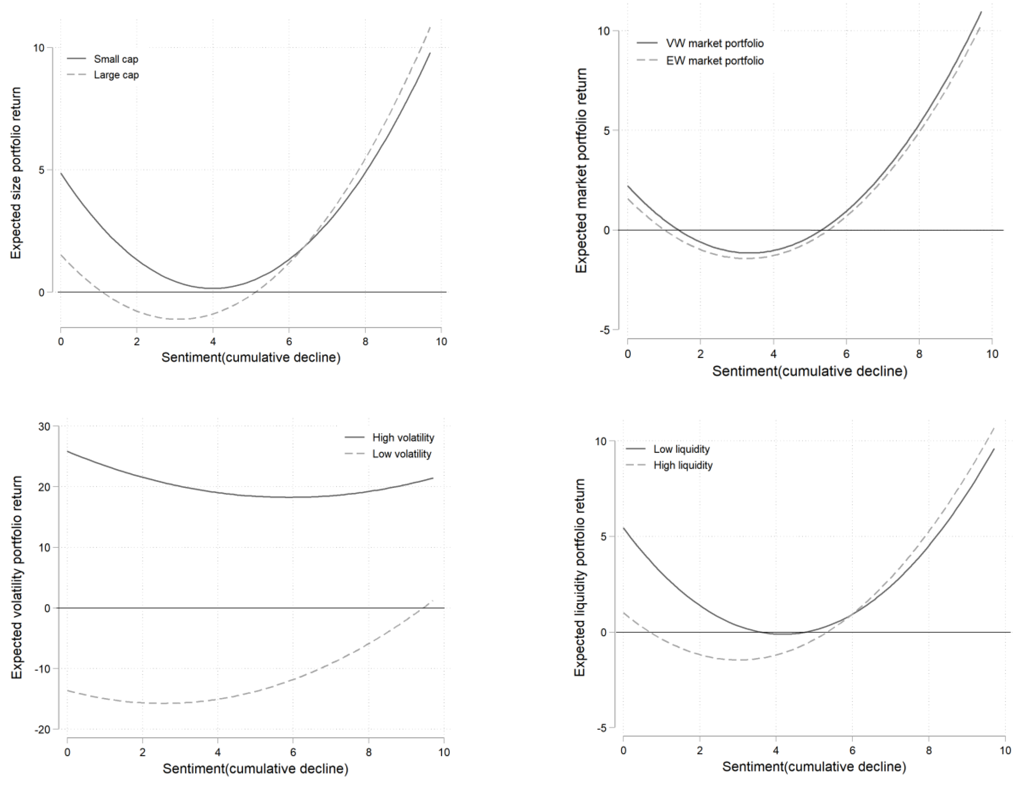
Finally, we present the results of the above empirical tests in the form of a fitting chart to help us better judge whether the conclusions of the theoretical part are supported by market evidence. According to Figure 5, the cumulative growth of sentiment can promote the sustained increase in returns at the initial stage, which leads to the formation of a bubble. When the sentiment and asset returns reach the peak, prices fall, which leads to a decrease in the asset returns, which is completely consistent with the conclusions obtained in Figure 1. In addition, the bubble generated by equal-weighted market portfolios consisting of small-cap stocks, low-liquidity stocks, and high-volatility stocks, which are mainly held by irrational individual investors, is larger and more difficult to burst (failing to intersect with axis 0), while the bubble generated by the value-weighted market portfolios that consist of large-cap stocks, high-liquidity stocks, and low-volatility stocks, which are mainly held by institutional investors, is smaller and easier to burst. The difference between the two is also highly consistent with the conclusion of the comparative static analysis in Figure 2. To date, we have further confirmed Proposition 1 of the theoretical model.
7.2.2. Cumulative Low Investor Sentiment and Asset Returns
We now switch the scenario from continuous high sentiment to continuous low sentiment, and we test Proposition 2 by discussing the relationship between cumulative sentiment decline and asset returns. All the variables remained unchanged, and we built the following empirical model:
According to Table 6, the signs of and are opposite to those in Table 5, which indicates that the cumulative depression of sentiment can have a negative impact on future portfolio returns in the short term, and can have a positive impact on future portfolio returns in the long term, which forms a negative bubble. At the aggregate level, the absolute values of and of the equal-weighted market portfolio are greater than those of the value-weighted market portfolio, which indicates that the bubble is more evident in the equal-weighted market portfolio, which again confirms the idea of Fama [17]. At the cross-sectional level, the small-cap stocks, low-liquidity stocks, and high-volatility stocks all produced more negative bubbles than large-cap stocks, high-liquidity stocks, and low-volatility stocks (by comparing the absolute values of and ), which confirmed the cross-sectional effect of the persistence of pessimistic sentiment on future portfolio returns. However, the cumulative pessimism of sentiment does not have a significant nonlinear impact on the returns of high-volatility-stock portfolios, which, in reality, may be explained by the short-selling constraint [18].
We discuss the results in depth in Table 6 in the form of a fitting graph. Figure 6 shows that cumulative pessimism can generate negative foam, whether in terms of aggregate or cross-sectional portfolios. Specifically, the size of the bubbles generated by the equal-weighted market portfolio of small-cap stocks, low-liquidity stocks, and high-volatility stocks is larger than that of the value-weighted market portfolio of large-cap stocks, high-liquidity stocks, and low-volatility stocks, which is consistent with the comparative static analysis results in Figure 4. Moreover, by comparing Figure 6 with Figure 5, we find that the impact of persistent optimism and pessimism on the same portfolio returns is asymmetric. Taking small-cap stocks as an example, when the sentiment experiences cumulative growth, the return rate of small-cap stocks increases from 2% to 9%, which is an increase of 7%. However, when the sentiment exhibits cumulative pessimism, the return of small-cap stocks decreases from 5% to about 0.1%, which is a decrease of 4.9%, which is the same as the difference between Figure 1 and Figure 3. Finally, for the portfolio of large-cap stocks, low-volatility stocks, and high-liquidity stocks, the inflection point of the parabola is located on the left side of the portfolio for small-cap stocks, high-volatility stocks, and low-liquidity stocks, which confirms that the bubbles of the portfolio of large-cap stocks, low-volatility stocks, and high-liquidity stocks can enter the burst stage earlier, which reflects the stronger arbitrage ability of the rational traders in such portfolios. The price deviation from the fundamental value can be corrected in a timely manner, which provides us with another explanatory path to verify the comparative static analysis in Figure 4.
So far, we have verified Proposition 2 in the theoretical model.
8. Conclusions
In this paper, we take the extrapolation belief as the micro-mechanism of sentiment feedback, and we discuss asset price bubbles from the theoretical to the empirical levels. According to the theoretical research, as positive (negative) fundamental information is injected into the market, asset prices increase (decrease), which stimulates an increase (decrease) in the sentiment of extrapolated investors and further pushes prices up (down). In this way, positive or negative bubbles are generated. Finally, the passage of the information shock gradually returns the sentiment of extrapolated investors to the rational level, which causes the bubbles to burst. In the above feedback process, the extrapolation belief always plays a central role.
At the empirical level, we first conducted a preliminary test on the proposition of the theoretical model. According to the results, an increase in investor sentiment reduces the information content of the asset price and aggravates the price volatility, while a decrease in investor sentiment will have the same effect, but it is not significant. This conclusion is consistent with the meaning behind the proposition that is generated by the theoretical model. Then, we took the sentiment feedback mechanism generated by the extrapolation belief as the starting point, discussed the relationship between the cumulative change in investor sentiment and future portfolio returns, and further attempted to verify the rationality of the theoretical model’s conclusions. According to the empirical results, the cumulative increase (decrease) in investor sentiment will push up (down) the future portfolio returns at the initial stage and push down (up) the future portfolio returns in the long term. This trend indicates a nonlinear relationship between the cumulative change in sentiment and future portfolio returns. This nonlinear relationship shows cross-sectional differences among different types of asset portfolios.
According to the research in this paper, irrational investors are vulnerable to the impact of historical price changes, which means that their trading behavior deviates from the rational framework. Rational investors will trade based on fundamental information to create asset–price stability. Therefore, the government’s regulatory authorities should strengthen the education of individual investors, enhance their awareness of the risks of stock market investment, and reduce the tendency of speculative trading. When the market substantially fluctuates, a risk warning should be issued through the media in a timely manner to reasonably channel the market sentiment fluctuations and reduce their impact on asset price fluctuations. In addition, the development of institutional investors should be increased, and individual investors should be encouraged to indirectly participate in the stock market by purchasing funds to share in the benefits of China’s economic growth.
We compared our findings with the existing literature. First, the extrapolated investor’s demand function in this paper is more in line with the characteristics of “trend extrapolation”. Let us take the extrapolated investor demand function established by De Long et al. [7] and Hu Changsheng et al. [19] as an example; the demand of such agent for risky assets in period t is only related to the price change in period , and cannot form the condition of “chasing trend” since only when the price changes continuously and in the same direction can the trend be generated. We use Barberis [2] for reference to propose this new extrapolated demand function. The extrapolated investor extrapolates the historical trend by weighting the price changes in the past several periods, and pays more attention to the recent price changes. Second, we do not introduce the short-selling constraint of Barberis et al. [11], since this condition cannot describe the negative bubbles caused by bad news, and thus cannot compare the two symmetrical situations of bubbles and negative bubbles. Third, different from the existing literature, we analyze the reasons for which fundamental traders fail to correct asset mispricing in a timely manner through the risk premium mechanism required by risk aversion, which leads to the emergence and expansion of bubbles, providing a new perspective for us to study the behavioral characteristics of rational traders. Finally, the disadvantage of the model described in this paper is that it does not discuss the trading volume during the bubble period from the theoretical and empirical levels. We hope to describe this scenario through the reform of market environment settings in future research, and enrich the research on bubbles.
Author Contributions
Conceptualization, C.C. and C.H.; methodology, H.Y.; software, C.C.; validation, C.C., C.H. and H.Y.; formal analysis, C.C. All authors have read and agreed to the published version of the manuscript.
Funding
This research was funded by [National Natural Science Foundation of China] grant number [71671134] and the [National Natural Science Foundation of China] grant number [72204099].
Data Availability Statement
Please contact the authors for data and software used in this study.
Conflicts of Interest
The authors declare no conflict of interest.
Appendix A
Proof of Lemma 1:
The CARA utility function optimization problem can be expressed as:
Due to the fact that consumption follows normal distribution (), its probability density function is as follows:
Due to the fact that the expression of the CARA utility function is , the expected utility can be written as follows:
where the integral term is the integral of the probability density function, and the integral value is 1; thus, the expected utility can be simplified as follows:
In summary, the problem of maximizing the expected utility can be transformed into:
Certificate completion. □
Proof of fundamental trader’s demand function:
For such agents, their trading decisions are made to maximize the expected utility of CARA: . We adopt the backward induction method, starting from the last trading day.
In , the expected wealth increase caused by each additional unit of risk assets is , and the expected future wealth is thus equal to . Due to the fact hat the information about has not yet appeared at this time, we can obtain:
Accordingly, , and we can solve the asset demand through the mean and variance of the expected wealth:
By calculating the first derivative, we obtain:
According to the market-clearing conditions:
In , the bounded rationality of the fundamental traders begins to play a role. Similarly, the expected wealth at this time is equal to , and we must infer to predict . Let us assume that fundamental traders do not try to predict changes in the demands of other investors but believe that extrapolated investors hold corresponding risky assets according to their market proportions: . Then, we have the following:
According to (A4):
The derivation still follows (A1):
According to the market-clearing conditions:
In , the expected wealth is: , and the conditional variance of the expected wealth is .
Finally, we obtain:
By combining (A2), (A7), and (A9), we obtain the general formula of the demand function of the fundamental traders for risk assets in a period ():
Certificate completion. □
Proof of extrapolated investor’s demand function:
The demand for risk assets formed by extrapolated investors according to extrapolation beliefs can also be solved through the CARA utility optimization:
We only need to follow the method of solving the demand function of the fundamental traders in a certain period to obtain the general formula of the demand function of the extrapolated investors:
In , the expected wealth is , and the conditional variance of the final wealth is . From this, we can obtain:
Unlike fundamental traders, extrapolated investors cannot infer the demands of other investors, and they will only form corresponding asset demands by forecasting future price changes in each period. Therefore, (A12) can be directly extended to:
The numerator of the above formula is significantly different from (A10). Extrapolated investors do not infer future price changes through dividends, but form beliefs about future price changes by extrapolating historical price changes:
Due to the fact that this paper constructs an economy starting from , the extrapolated investors cannot extrapolate at . At , extrapolation is not possible, but the initial value of the extrapolation belief can be obtained. Let us make constant.
Then, we investigate the scenario of (A14) when :
At , the extrapolated investors can extrapolate the price change between and :
Let us substitute (A15) into the above equation to obtain:
At :
At :
According to (A15)–(A19), we can conclude:
Then, we can obtain the demand function of the extrapolated investors according to the extrapolation beliefs:
Certificate completion. □
References
- Barberis, N.; Thaler, R. A Survey of Behavioral Finance. In Handbook of The Economics of Finance; Elsevier: Amsterdam, The Netherlands, 2003; Volume 1, pp. 1053–1128. [Google Scholar] [CrossRef]
- Barberis, N. Psychology-Based Models of Asset Prices and Trading Volume. In Handbook of Behavioral Economics: Applications and Foundations 1; Elsevier: Amsterdam, The Netherland, 2018; Volume 1, pp. 79–175. [Google Scholar] [CrossRef]
- Giglio, S.; Kelly, B. Excess Volatility: Beyond Discount Rates. Q. J. Econ. 2018, 133, 71–127. [Google Scholar] [CrossRef]
- Augenblick, N.; Lazarus, E. Restrictions on Asset-Price Movements under Rational Expectations: Theory and Evidence. 2018. Available online: https://ssrn.com/abstract=3436384 (accessed on 7 March 2022).
- Campbell, J.Y.; Shiller, R.J. The Dividend-Price Ratio and Expectations of Future Dividends and Discount Factors. Rev. Financ. Stud. 1988, 1, 195–228. [Google Scholar] [CrossRef] [Green Version]
- Cutler, D.M.; Poterba, J.M.; Summers, L.H. Speculative Dynamics and the Role of Feedback Traders. In The American Economic Review: Papers and Proceedings; National Bureau of Economic Research Cambridge: Cambridge, MA, USA, 1990; Volume 80, pp. 63–68. Available online: http://www.nber.org/papers/w3243 (accessed on 7 March 2022).
- De Long, J.B.; Shleifer, A.; Summers, L.H.; Waldman, R.J. Positive Feedback Investment Strategies and Destabilizing Rational Speculation. J. Financ. 1990, 45, 375–395. [Google Scholar] [CrossRef] [Green Version]
- Hong, H.; Stein, J.C. A Unified Theory of Underreaction, Momentum Trading, and Overreaction in Asset Markets. J. Financ. 1999, 54, 2143–2184. [Google Scholar] [CrossRef] [Green Version]
- Barberis, N.; Shleifer, A. Style Investing. J. Financ. Econ. 2003, 68, 161–199. [Google Scholar] [CrossRef] [Green Version]
- Barberis, N.; Greenwood, R.; Jin, L.; Shleifer, A. X-CAPM: An Extrapolative Capital Asset Pricing Model. J. Financ. Econ. 2015, 115, 1–24. [Google Scholar] [CrossRef] [Green Version]
- Barberis, N.; Greenwood, R.; Jin, L.; Shleifer, A. Extrapolation and Bubbles. J. Financ. Econ. 2018, 129, 203–227. [Google Scholar] [CrossRef] [Green Version]
- Liao, J.; Peng, C.; Zhu, N. Extrapolative Bubbles and Trading Volume. Rev. Financ. Stud. 2022, 35, 1682–1722. [Google Scholar] [CrossRef]
- Xiong, W.; Yu, J. The Chinese Warrants Bubble. Am. Econ. Rev. 2011, 101, 2723–2753. [Google Scholar] [CrossRef] [Green Version]
- Baker, M.; Wurgler, J. Investor Sentiment in the Stock Market. J. Econ. Perspect. 2007, 21, 129–152. [Google Scholar] [CrossRef] [Green Version]
- Hu, C.S.; Chi, Y.C. Research on Investor Sentiment and Abnormal Volatility of Asset Price. Master’s Thesis, Wuhan University, Wuhan, China, 2014. [Google Scholar]
- Berger, D.; Turtle, H.J. Sentiment Bubbles. J. Financ. Mark. 2015, 23, 59–74. [Google Scholar] [CrossRef]
- Liu, Y.; Yang, A.; Zhang, J.; Yao, J. An Optimal Stopping Problem of Detecting Entry Points for Trading Modeled by Geometric Brownian Motion. Comput. Econ. 2020, 55, 827–843. [Google Scholar] [CrossRef]
- Mendel, B.; Shleifer, A. Chasing Noise. J. Financ. Econ. 2012, 104, 303–320. [Google Scholar] [CrossRef]
- Hu, C.S.; Peng, Z.; Chi, Y.C. Feedback trading, Trading inducement and Asset price behavior. Econ. Res. J. 2017, 5, 189–202. [Google Scholar]
- Greenwood, R.; Shleifer, A. Expectations of Returns and Expected Returns. Rev. Financ. Stud. 2014, 27, 714–746. [Google Scholar] [CrossRef] [Green Version]
- Loewenstein, M.; Willard, G.A. The limits of investor behavior. J. Financ. 2006, 61, 231–258. [Google Scholar] [CrossRef]
- Chen, C.; Hu, C.S. Does Feedback Trading Cause the Instability of Rational Speculation? Forecasting 2021, 40, 53–59. [Google Scholar]
- Robert, S. Irrational Exuberance. Master’s Thesis, China Renmin University, Bejing, China, 2016. [Google Scholar]
- Stambaugh, R.F.; Yu, J.; Yuan, Y. Arbitrage Asymmetry and the Idiosyncratic Volatility Puzzle. J. Financ. 2015, 70, 1903–1947. [Google Scholar] [CrossRef] [Green Version]
- Hu, C.S.; Chen, C.; Chi, Y.C. Up and Down of Stock Movement is Caused by Sentiment: Sentiment Beta and Stock Market Style Dynamic Preference Shift. J. Stat. Inform. 2020, 35, 71–79. [Google Scholar]
- Sibley, S.E.; Wang, Y.; Xing, Y.; Zhang, X. The information content of the sentiment index. J. Bank. Financ. 2016, 62, 64–179. [Google Scholar] [CrossRef]
- Campbell, J.Y.; Lettau, M.; Malkiel, B.G.; Xu, Y. Have individual stocks become more volatile? An empirical exploration of idio-syncratic risk. J. Financ. 2001, 56, 1–43. [Google Scholar] [CrossRef]
- Brandt, M.W.; Brav, A.; Graham, J.R.; Kumar, A. The Idiosyncratic Volatility Puzzle: Time Trend or Speculative Episodes. Rev. Financ. Stud. 2010, 23, 863–899. [Google Scholar] [CrossRef]
- Llorente, G.; Michaely, R.; Saar, G.; Wang, J. Dynamic volume-return relation of individual stocks. Rev. Financ. Stud. 2002, 15, 1005–1047. [Google Scholar] [CrossRef]
- Markowitz, H. The Utility of Wealth. J. Polit. Econ. 1952, 60, 151–158. [Google Scholar] [CrossRef]
- Fama, E. Market Efficiency, Long Term Returns, and Behavioral Finance. J. Financ. Econ. 1998, 49, 283–306. [Google Scholar] [CrossRef]
Figure 1.
Asset price bubbles under the impact of good news.
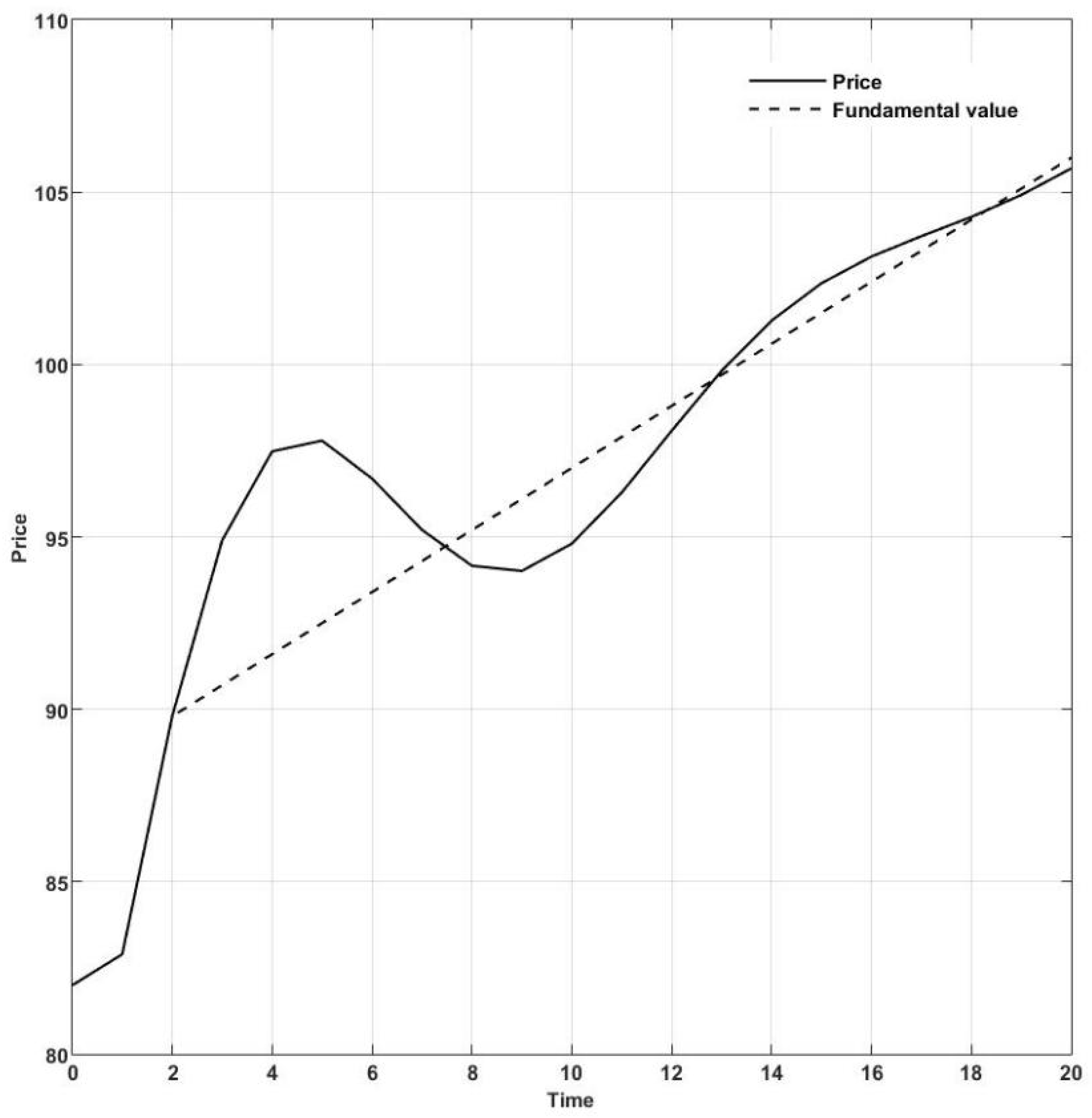
Figure 2.
Comparative static analysis (the impact of good news).
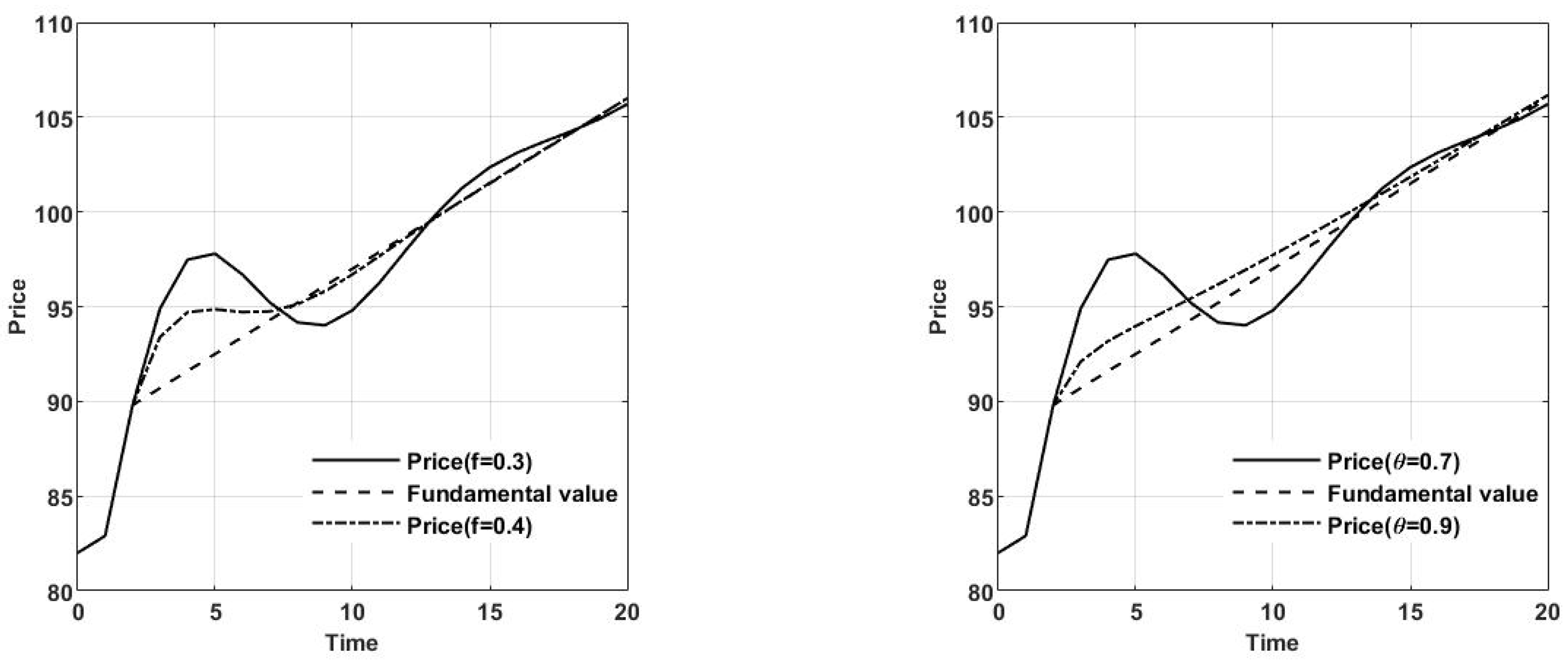
Figure 3.
Asset price bubbles under the impact of bad news.
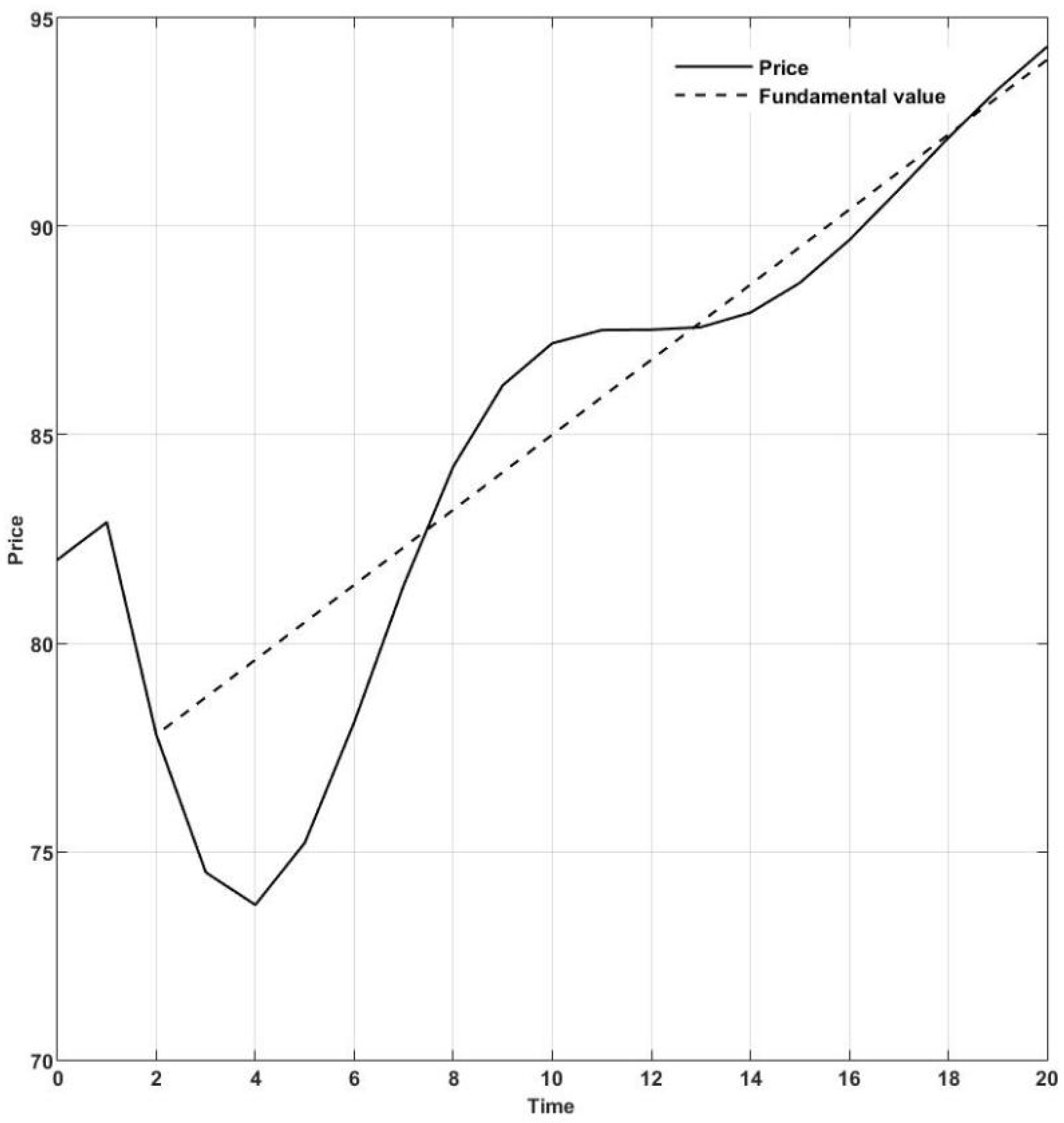
Figure 4.
Comparative static analysis (the impact of bad news).

Figure 5.
Cumulative growth in sentiment and portfolio returns (fitting).
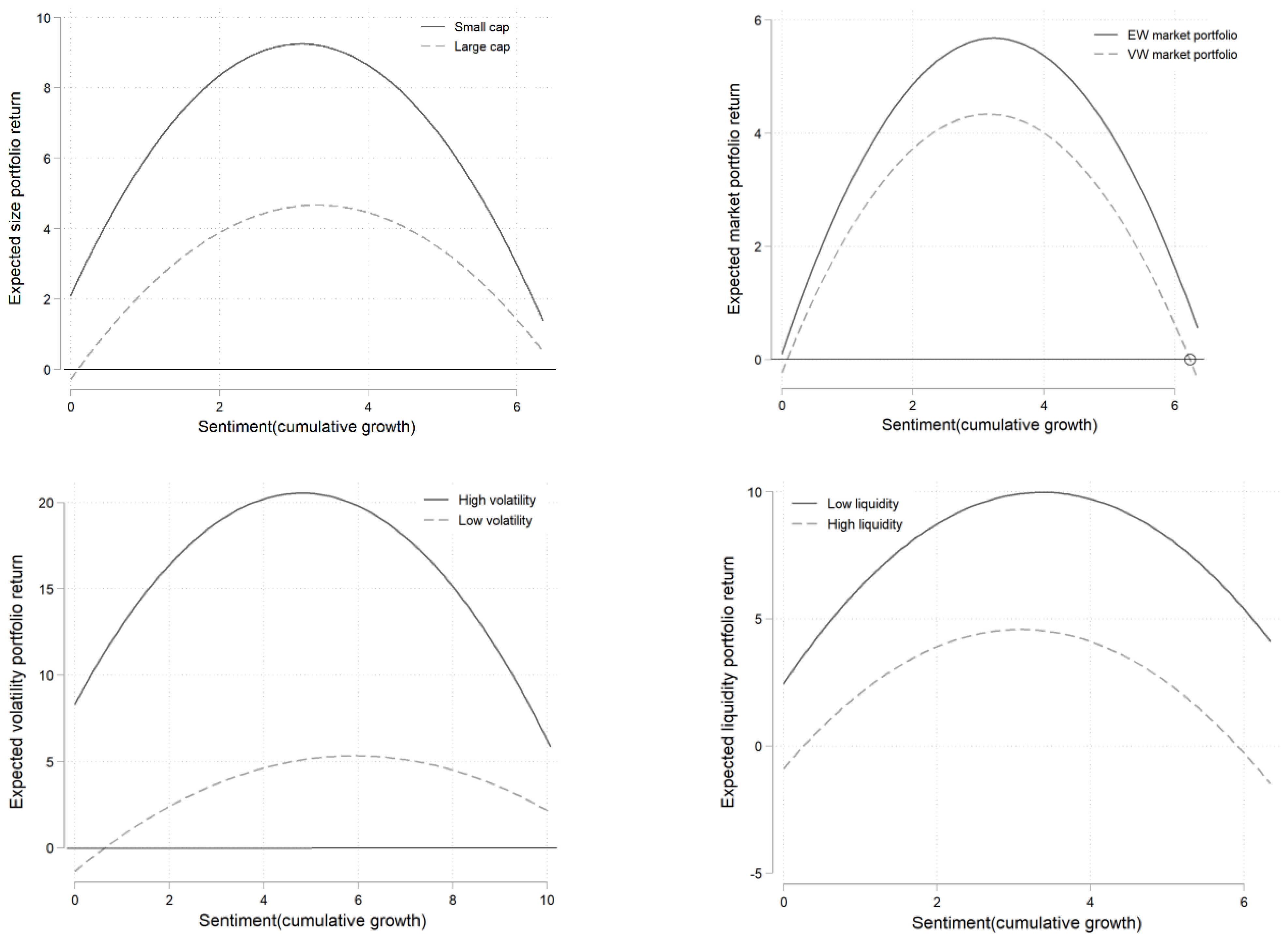
Figure 6.
Cumulative decline in sentiment and portfolio returns (fitting).

Table 1.
Parameter settings.
| Parameter | Value |
|---|---|
| 100 | |
| 3 | |
| 1 | |
| 20 | |
| 0.3 | |
| 0.7 | |
| 0.1 | |
| 0.7 |
Table 2.
Descriptive statistics.
| Variable | Mean | Median | Standard Deviation | Minimum | Maximum |
|---|---|---|---|---|---|
| −14.060 | −13.060 | 70.312 | −3490.523 | 11,291.77 | |
| −15.601 | −15.962 | 17.203 | −86.378 | 44.398 | |
| Investor sentiment index | 0 | −0.197 | 1.362 | −4.200 | 3.983 |
| Unemployment rate | 4.089 | 4.1 | 0.132 | 3.61 | 4.3 |
| Illiquidity | 0.284 | 0.121 | 0.327 | 0.025 | 1.864 |
| Market volatility | 0.015 | 0.013 | 0.008 | 0.003 | 0.044 |
| Real GDP growth rate | 9.280 | 9.4 | 2.353 | 6.2 | 14.3 |
| Individual-share ROE synchronization | 0.462 | 0.823 | 0.499 | −5.070 | 3.620 |
| Market ROE synchronization | 2.102 | 2.355 | 0.933 | −0.038 | 4.111 |
Table 3.
Investor sentiment and prevalence of informed trading.
| −5.319 ** | |
| (−2.42) | |
| −2.299 | |
| (−0.60) | |
| −1.603 | |
| (−1.02) | |
| −0.255 | |
| (−1.12) | |
| 0.001 | |
| (1.23) | |
| 3.355 | |
| (1.28) | |
| 3.224 | |
| (0.15) | |
| 0.065 | |
Note: *, **, and *** represent significance levels of 10%, 5%, and 1%, respectively. We provide the t-statistics adjusted by Newey West in the parentheses.
Table 4.
Descriptive statistics.
| Variable | Mean | Standard Deviation | Minimum | Maximum |
|---|---|---|---|---|
| Small cap | 3.763 | 13.046 | −22.862 | 97.46 |
| Large cap | 0.9 | 8.365 | −28.666 | 32.502 |
| Low liquidity | 4.171 | 12.048 | −23.399 | 89 |
| High liquidity | 0.425 | 9.109 | −32.06 | 31.589 |
| High volatility | 10.884 | 14.311 | −26.616 | 62.595 |
| Low volatility | −0.074 | 7.607 | −23.406 | 48.249 |
| Investor sentiment change index | 0 | 1.522 | −9.701 | 10.071 |
| Cumulative high sentiment index | 0.795 | 1.494 | 0 | 10.071 |
| Cumulative low sentiment index | −0.776 | 1.388 | −9.701 | 0 |
| Risk-free rate | 0.002 | 0.001 | 0.001 | 0.003 |
| Value-weighted market return | 0.861 | 7.959 | −26.809 | 29.604 |
| Equal-weighted market return | 1.416 | 9.477 | −28.836 | 34.416 |
Table 5.
Sentiment cumulative growth and portfolio returns.
| Portfolio | (1) Intercept | (2) | (3) |
|---|---|---|---|
| EMkt | 0.178 | 3.372 ** | −0.520 * |
| (0.23) | (2.45) | (−1.86) | |
| VMkt | −0.167 | 2.612 ** | −0.438 * |
| (−0.26) | (2.32) | (−1.91) | |
| Small | 2.109 ** | 4.616 ** | −0.745 * |
| (1.96) | (2.43) | (−1.93) | |
| Large | −0.281 | 2.990 ** | −0.451 * |
| (−0.41) | (2.45) | (−1.82) | |
| Lowliq | −1.221 ** | 4.472 ** | −0.663 * |
| (2.47) | (2.56) | (−1.87) | |
| Highliq | −0.881 | 3.534 *** | −0.572 ** |
| (−1.17) | (2.66) | (−2.12) | |
| Highvol | 9.039 *** | 5.144 ** | −0.799 * |
| (7.68) | (2.48) | (−1.90) | |
| Lowvol | −1.221 * | 3.308 *** | −0.491 ** |
| (−1.94) | (2.75) | (−2.18) |
Note: *, **, and *** represent significance levels of 10%, 5%, and 1%, respectively. We provide the t-statistics adjusted by Newey West in the parentheses.
Table 6.
Cumulative sentiment decline and portfolio returns.
| Portfolio | (1) Intercept | (2) | (3) |
|---|---|---|---|
| EMkt | 2.221 *** | −2.013 ** | 0.300 * |
| (2.84) | (−2.00) | (1.91) | |
| VMkt | 1.580 ** | −1.847 ** | 0.283 ** |
| (2.41) | (−2.19) | (2.15) | |
| Small | 4.857 *** | −2.357 ** | 0.295 ** |
| (4.22) | (−2.04) | (2.04) | |
| Large | 1.532 ** | −1.701 * | 0.274 ** |
| (2.29) | (−1.87) | (2.39) | |
| Lowliq | 5.441 *** | −2.657 ** | 0.318 ** |
| (5.14) | (−2.39) | (2.33) | |
| Highliq | 1.011 | −1.637 * | 0.271 ** |
| (1.41) | (1.65) | (2.18) | |
| Highvol | 11.969 *** | −1.729 | 0.118 |
| (10.12) | (−1.13) | (0.50) | |
| Lowvol | 0.588 | −1.786 ** | 0.284 ** |
| (0.94) | (−2.22) | (2.25) |
Note: *, **, and *** represent significance levels of 10%, 5%, and 1%, respectively. We provide the t-statistics adjusted by Newey West in the parentheses.
Publisher’s Note: MDPI stays neutral with regard to jurisdictional claims in published maps and institutional affiliations. |
© 2022 by the authors. Licensee MDPI, Basel, Switzerland. This article is an open access article distributed under the terms and conditions of the Creative Commons Attribution (CC BY) license (https://creativecommons.org/licenses/by/4.0/).
Share and Cite
MDPI and ACS Style
Chen, C.; Hu, C.; Yao, H. Behavioral Framework of Asset Price Bubbles: Theoretical and Empirical Analyses. Systems 2022, 10, 251. https://doi.org/10.3390/systems10060251
AMA Style
Chen C, Hu C, Yao H. Behavioral Framework of Asset Price Bubbles: Theoretical and Empirical Analyses. Systems. 2022; 10(6):251. https://doi.org/10.3390/systems10060251
Chicago/Turabian StyleChen, Cong, Changsheng Hu, and Hongxing Yao. 2022. "Behavioral Framework of Asset Price Bubbles: Theoretical and Empirical Analyses" Systems 10, no. 6: 251. https://doi.org/10.3390/systems10060251
Note that from the first issue of 2016, this journal uses article numbers instead of page numbers. See further details here.