

Improving Acceptability of Cost Savings Allocation in Ridesharing Systems Based on Analysis of Proportional Methods

Department of Computer Science and Information Engineering, Chaoyang University of Technology, Taichung 413310, Taiwan
Systems 2023, 11(4), 187; https://doi.org/10.3390/systems11040187
Submission received: 7 February 2023
/
Revised: 31 March 2023
/
Accepted: 3 April 2023
/
Published: 6 April 2023
(This article belongs to the Special Issue Circular Economy Systems: Design, Use, and Innovation)
Abstract
:Due to its potential for cutting down energy consumption, sharing transport costs, and reducing negative impacts on the environment, ridesharing has been adopted as a viable model by many cities all over the world to achieve sustainability goals. Although there have been many studies on ridesharing systems, most of these studies have focused on the optimization of performance directly linked to saving energy consumption costs or travel distance. The methods used to divide the cost savings among the ridesharing participants have been less explored. In practice, proportional methods are commonly used to allocate cost savings in ridesharing systems. However, the effectiveness of proportional methods has not been well studied. The goal of this paper is to study and compare three proportional cost savings allocation methods to provide a guideline for choosing an effective method based on an analysis of the properties and performance in terms of the number of acceptable rides and the number of ridesharing participants. The properties were verified by experimental results. This study showed that how cost savings are divided among ridesharing participants has a significant influence on participants’ willingness to adopt the ridesharing transport mode. The properties and experimental results provide a rule and principle that can be used by policy makers and service providers to move towards their sustainability goals by promoting ridesharing through adopting the right proportional cost savings allocation method in ridesharing systems.
1. Introduction
Global warming is mainly due to excessive emissions of greenhouse gases (GHG). GHG emissions are closely related to energy consumption. The share of energy consumption in the transport sector has increased steadily from 8.6% in 1973 to 25% in 2022 [1,2]. In particular, the total energy consumption in the U.S. for transporting people and goods was about 28% in 2021 [3]. The circular economy [4] is an economic paradigm that aims to minimize energy consumption/pollution/waste, extend product lifecycles, and promote the sharing of resources to achieve the Sustainable Development Goals. The sharing economy, which is built on the sharing of resources to improve underutilized resources, is an important pillar that can contribute to the circular economy. The sharing economy [5] has attracted the attention of practitioners and researchers from relevant sectors and communities due to its potential benefits to improve efficiency and sustainability based on the sharing of resources. It sparks new research problems under the sharing paradigm. For example, Xu et al. presented a multi-objective optimization model for task–resource allocation in a multi-stage resource leveling problem in a sharing logistics network [6]. The objectives considered in [6] include total cost, total duration, resource efficiency, and stability for traditional resource providers. The results showed that the improved algorithm proposed in this paper can effectively solve the problem.
In the transport sector, the idle time of cars is over 90%. Only 1.5 seats are occupied for typical cars with five seats [7]. Therefore, cars are a significantly underutilized resource. To reduce its environmental footprint, the transport sector will need to improve its utilization of resources. Innovative shared mobility models such as ridesharing, ride-hailing and carsharing can help improve resource utilization in the transport sector to achieve the goal of the circular economy through sharing. Due to a lack of a broadly accepted definition of the term “shared mobility” in the academic literature, Castellanos et al. proposed a taxonomy for shared mobility to capture the interactions between digital technology and transport as well as the sharing economy concept [8]. Cost savings provide a strong incentive for the shared mobility mode. Therefore, the optimization of performance metrics relevant to cost savings in shared mobility systems has been extensively studied in the literature [9].
In the sharing economy, ridesharing [10], ride-hailing [11], and carsharing [12] are three types of emerging transport modes facilitated through advances in online platforms. Ridesharing allows multiple riders to get to their destinations on-demand by sharing a single vehicle that makes multiple stops to pick up and drop off riders. That is, the driver of the ridesharing vehicle shares a ride with the riders. In ride-hailing, a rider hires a personal driver to take him/her to the designated destination. In ride-hailing, the transportation vehicle is not shared with any other riders, nor does it make several stops on the way to the destination of the rider. Carsharing allows people to exclusively use a car temporarily based on payment for usage of the car. Carsharing makes it possible for people to use a car without owning it. This paper focuses on ridesharing.
Due to the potential benefits to cut down energy consumption, share transport costs, and reduce the negative impact on the environment, ridesharing has been adopted as a viable model by many cities and organizations all over the world to mitigate GHG emissions and achieve sustainability goals. Ridesharing has been adopted by companies such as Uber, Lyft, and Didi as well as universities [13,14]. For this reason, ridesharing has attracted the attention of researchers and has sparked new challenges as well as many interesting and important research subjects in the relevant communities over the last two decades. These ridesharing research challenges and subjects were discussed in the review papers by Furuhata et al. [15] and Agatz et al. [16]. Interesting questions such as (1) what factors make it more likely for ridesharing to occur in a place? (2) what factors make people use ridesharing services? [17], (3) what are the determinants of ridesharing? [18], (4) how can people’s preferences relevant to ridesharing be measured? [19], (5) how are travelers’ ridesharing decisions affected by social networks? [20], (6) how can cost savings be maximized [21] or travel distance in ridesharing systems reduced? [22], (7) how can monetary incentive be maximized? [23] and (8) how can the enjoyability of people on a shared ride be improved? [24]. The incorporation of social preferences into ridesharing decisions was studied by Saisubramanian et al. in [25] and the consideration of trust in the ridesharing system was studied by Hsieh in [26]. A study on sharing rides with friends was available in the work [27] by Bistaffa et al. A review of user behaviors/characteristics as well as social-economic impacts of the shared transport mode was available in the paper [28] by Sun et al. Recent developments in studies on ridesharing can be found in the paper [29] by Hyland and Mahmassani.
Although cities may benefit from ridesharing, stakeholders such as drivers and riders may adopt the ridesharing transport mode for a variety of reasons. People used to drive their own cars may not accept ridesharing due to inconvenience, detours, and the extra time needed to share with other riders. Riders used to commute with public transport may not accept ridesharing if the benefits do not outweigh the disadvantages such as unreliability and safety. For these reasons, studies on how to provide incentive and eliminate ridesharing barriers is an important issue.
The report by Hansen & Sener indicated that ridesharing is more likely to be considered by lower incomes public transit users [30]. Hence, time and cost are two important factors for users to determine whether to choose the ridesharing mode. The study of Waerden et al. [31] also indicated that the two determining factors for users to accept ridesharing are cost and time. Incentives for users to adopt ridesharing can be classified into financial incentives, social incentives, and accessibility incentives. Accessibility incentives refer to the improvement in convenience due to the flexibility of ridesharing in comparison with public transport in terms of time and space. Social incentives refer to enjoyability and trust in ridesharing. Financial incentives refer to the monetary incentives offered by ridesharing. These issues have been studied in the literature. Among these three types of incentives, financial incentives are essential as cost reduction is a common feature expected by the users. Without providing financial incentives, ridesharing would not be attractive. Financial incentives are due to the reduction in transport costs or cost savings due to ridesharing. For the given cost savings, an important issue is to properly divide savings in cost among the ridesharing participants.
In the literature, many methods were proposed to allocate cost or cost savings in different applications [32]. Proportional methods [33], nucleolus [34] and the Shapley value [35] were three well-known methods for allocating cost/savings among players. Both the nucleolus and Shapley value methods suffer from complexity issues [36,37]. The study of Levinger et al. [38] shows that there is no polynomial time algorithm for computing the Shapley value in ridesharing problems. The nucleolus approach was also applied by Lu and Quadrifoglio in allocating cost/savings among ridesharing participants [39]. However, it is very difficult to compute the nucleolus for the n-player game as the size of the characteristic function grows exponentially and the difficulty to compute the nucleolus grows with .
Proportional methods are one of the most widely used approaches in practice to allocate cost/savings in ridesharing systems [40,41,42,43] due to its simplicity and computational efficiency. For example, a pricing method based on the proportional method was proposed by Cipolina-Kun et al. in [40] for a ridesharing system considering meeting points. In the work by Wang et al. [41], a proportional method was proposed to divide the cost savings of sharing systems equally between the driver and the rider on the ride. In the paper by Agatz et al. [42], the cost savings are allocated to the driver and the rider proportionally to their respective travel distance. In the study [43] by Hsieh et al., a method to allocate cost savings among the ridesharing information provider, ridesharing passengers, and drivers was defined. The amount allocated to each passenger and each driver was proportional to their original travel costs when they travel alone.
In the previous study by Hsieh [44], it was shown that the ways to divide the cost savings among the ridesharing participants had significant influence on the participants’ willingness to adopt the ridesharing transport mode. In [44], Hsieh unveiled several properties indicating that the ways to divide cost savings among participants will influence the number of acceptable rides in ridesharing systems. The properties studied in [44] by Hsieh were based on the assumption that the minimal expected rewarding rate for drivers and that of passengers are the same. Based on this assumption, a comparative study of three schemes proposed in [41,42,43] to divide cost savings among participants was done by Hsieh through analysis in [44]. However, drivers and passengers may have different minimal expected rewarding rates in the real world. It is important to consider the situation that the minimal expected rewarding rate for drivers and that of passengers may be different in analysis of the properties. A study on the situation in which there is an assumption that the minimal expected rewarding rate for drivers may be different from that of passengers is still lacking. Motivated by the deficiency in the existing studies, this study aims to explore relevant properties of schemes to divide savings of cost among participants under the assumption that the minimal expected rewarding rate for drivers and that of passengers may not be the same.
In this study, the combinatorial double auction model proposed by Hsieh et al. [43] was extended for ridesharing systems and its properties were analyzed using the assumption that the minimal expected rewarding rate for drivers and that of passengers may not be the same. The performance indices of the number of acceptable rides and the number of ridesharing participants accepting the rides were compared by analyzing several properties of three proportional methods with the assumption that the minimal expected rewarding rate for drivers and for passengers may not be the same. The properties were verified by experimental results.
One of the contributions of this paper is to provide conditions for choosing an effective allocation method in ridesharing systems. The conditions were identified without assuming that the minimal expected rewarding rate for drivers and that of passengers would be the same. Therefore, this paper is different from the work [44] by Hsieh. Another contribution of this paper is to compare the number of ridesharing participants accepting ridesharing in addition to the number of acceptable rides based on an analysis of the properties. The third contribution of this paper is to provide results of experiments for verification of the properties analyzed in this paper. The properties and experimental results provide a rule and principle that can be used by policy makers and service providers to move towards their sustainability goals by promoting ridesharing through an adoption of the right proportional cost savings allocation method in ridesharing systems.
The rest of this paper is organized as follows. In Section 2, the ridesharing decision model and three proportional methods to allocate cost savings due to reduction in energy consumption in ridesharing systems will be reviewed. Several properties that characterize the performance of the three proportional methods to allocate savings of cost will be presented in Section 3. These properties will be verified through experiments and the results will be presented in Section 4. The results of the experiments will be summarized and discussed in Section 5. This paper will be concluded in Section 6.
2. Proportional Methods to Divide Cost Savings among Ridesharing Participants
In this section, the cost savings optimization problem in ridesharing systems will be described and three proportional methods for cost savings allocation will be reviewed. Several interesting properties of the three proportional methods will be analyzed in Section 3.
Before reviewing the three proportional methods for cost savings allocation, the ridesharing problem formulation is introduced first. Table 1 shows the symbols/variables/parameters used in the problem formulation.
The ridesharing problem is used to determine the set of drivers and passengers that optimize the performance, such as transport cost savings, while meeting the requirements of the drivers and the passengers. In this paper, it is assumed that the combinatorial double auction based ridesharing problem formulation proposed in [43] is used. This problem can be modeled as a combinatorial double auction problem in which drivers play the role of sellers and passengers play the role of buyers. In this decision model, a driver can submit bids, denoted by , . A passenger can submit one bid, denoted by . Please refer to Table 1 for the details of and . The decision variables of this problem include the driver ’s decision variable and passenger ’s decision variable , where , and .
As this study focuses on the allocation of cost savings due to the reduction in energy consumption in ridesharing systems, the objective function to be maximized in the combinatorial double auction based ridesharing problem is defined in Equation (1), where is the original cost of passengers (without ridesharing), is the original cost of drivers (without ridesharing) and is the original cost of drivers with ridesharing. The combinatorial double auction based ridesharing problem is formulated as an integer programming problem in Equation (1) through Equation (6). This is a typical constrained optimization problem with constraints (2) and (3) as the demand and supply constraints, constraint (4) as the cost savings constraint, and constraint (5) as the drivers’ single winning bid constraint. The optimization problem is to determine the values of decision variables and of drivers and passengers.
s.t.
Many solution algorithms (e.g., the ten algorithms proposed in [21,26] by Hsieh and the algorithm developed in [43] by Hsieh et al.) have been developed to solve the problem to maximize cost savings due to energy/fuel consumption. The allocation of cost savings in the ridesharing system is to allocate the cost savings among the stakeholders in ridesharing systems. In typical ridesharing systems, passengers, drivers, and the ridesharing information provider are the stakeholders. A method to allocate cost savings is defined by assigning the share values , and to passengers, drivers, and the ridesharing information provider, respectively, where . Share values are determined by the ridesharing system operators.
In ridesharing systems, passengers and drivers have expectations for a minimal rewarding rate due to properly allocated cost savings. Therefore, a method used to allocate cost savings will influence the acceptance of ridesharing. In the literature, three proportional methods, the Fifty-Fifty (FF) Method, proposed by Wang et al. in [41], the Local Proportional (LP) Method, proposed by Agatz et al. in [42] and the Global Proportional (GP) Method, proposed by Hsieh in [43], were defined to allocate the cost savings among the stakeholders in ridesharing systems. The Fifty-Fifty Method assumes that there is one driver and one passenger in a ride and divides the cost savings equally between the driver and the passenger in each matched ride. The way to divide the cost savings between the driver and the passenger on a ride in the Local Proportional Method is proportional to the travel distance of the driver and the passenger. The Global Proportional Method divides the cost savings among the ridesharing participants based on the ratio of an individual participant’s bid price to the overall price of the matched bids. These three methods are defined in Table 2. For the Fifty-Fifty Method, the share values for the stakeholders are defined in Equations (7)–(9). For the Local Proportional Method, the share values for the stakeholders are defined in Equations (10)–(14). The share values for the stakeholders of the Global Proportional Method are defined in Equations (15)–(17).
In this paper, it is assumed that drivers and passengers have expectations for a rewarding rate due to cost savings and their expectations for rewarding rates are described by the minimal expected rewarding rates. The minimal expected rewarding rate for drivers and the minimal expected rewarding rate for passengers are defined as follows.
Definition1.
Minimal Expected Rewarding Rates.
The minimal expected rewarding rates are the minimal expectations for drivers and passengers to accept ridesharing. The minimal expected rewarding rate for drivers is denoted by and the minimal expected rewarding rate for passengers is denoted by .
The minimal expected rewarding rates can be determined by an online questionnaire.
Based on the definition above, ridesharing will be acceptable to drivers and passengers only when their minimal expected rewarding rates can be satisfied.
A ride will be acceptable for a driver only if the rewarding rate is greater than or equal to the minimal expected rewarding rate of drivers. A ride will be acceptable for a passenger only if the rewarding rate is greater than or equal to the minimal expected rewarding rate of passengers. Therefore, an acceptable ride is defined as follows.
Definition 2.
Acceptable Ride.
A ride is said to be an acceptable ride if the rewarding rate for the driver on the ride is greater than or equal to the minimal expected rewarding rate and the rewarding rate for the passenger on the ride is greater than or equal to the minimal expected rewarding rate .
Based on the above definition, the three methods will be analyzed in the next section.
3. Comparison with Proportional Allocation Methods
In this section, the proportional allocation methods in the literature will be compared. The performance indices for comparing different methods include total passengers on the acceptable rides, total participants on the acceptable rides, and total acceptable rides. Four properties will be presented to compare the performance of the three proportional methods defined in Section 2. These four properties will be presented through analysis taken one by one in this section.
Property 1 characterizes the condition under which the performance of the Global Proportional Method is either as good as or better than that of the Local Proportional Method.
Lemma 1.
The rewarding rate of shared rides under the Global Proportional Method is greater than or equal to the lowest rewarding rate of the shared rides under the Local Proportional Method.
Proof of Lemma 1.
Please refer to Appendix A. □
Property 1.
Let the minimal expected rewarding rate for all winning drivers be and the minimal expected rewarding rate for all winning passengers be . If the rewarding rate under the Global Proportional Method is greater than , the number of acceptable rides, the number of passengers on the acceptable rides, and the number of participants on the acceptable rides under the Global Proportional Method are greater than or equal to those under the Local Proportional Method.
Proof of Property 1.
Let be a solution obtained by solving the ridesharing problem. In the Global Proportional Method, the rewarding rate for passenger is . The rewarding rate for passenger is = . In the Global Proportional Method, the rewarding rate for driver is . The rewarding rate for driver is . Therefore, the rewarding rate for each passenger and each driver is the same. If the rewarding rate under the Global Proportional Method is greater than , then , and .
In this case, the number of acceptable rides under the Global Proportional Method is . The number of passengers on the acceptable rides under the Global Proportional Method is . The number of ridesharing participants on the acceptable rides under the Global Proportional Method is .
The set of drivers accepting ridesharing under the Global Proportional Method is defined in Equation (18):
The set of passengers accepting ridesharing under the Global Proportional Method is defined in Equation (19):
If the Local Proportional Method is used, the rewarding rate for passenger is , where . The rewarding rate for passenger is . If the Local Proportional Method is used, the rewarding rate for driver is , where .
The rewarding rate for driver is .
For driver to transport the set of passengers in , the following conditions must be satisfied: and .
The set of drivers accepting ridesharing under the Local Proportional Method is defined in Equation (20).
According to Lemma 1, the rewarding rate under the Global Proportional Method is greater than or equal to the lowest rewarding rate under the Local Proportional Method. So .
That is, the number of acceptable shared rides under the Local Proportional Method is .
The set of passengers accepting ridesharing under the Local Proportional Method is defined in Equation (21).
According to Lemma 1, the rewarding rate under the Global Proportional Method is greater than or equal to the lowest rewarding rate under the Local Proportional Method. So .
That is, the number of passengers on the acceptable shared rides under the Local Proportional Method is .
In addition, the number of participants on the acceptable rides under the Local Proportional Method is .
This completes the proof. □
Property 2 characterizes the condition under which the performance of the Local Proportional Method is either as good as or outperforms that of the Global Proportional Method.
Property 2.
Let the minimal expected rewarding rate for all winning drivers be and the minimal expected rewarding rate for all winning passengers be . If the rewarding rate under the Global Proportional Method is less than , the number of acceptable rides, the number of passengers on the acceptable rides and the number of participants on the acceptable rides under the Local Proportional Method are greater than or equal to those under the Global Proportional Method.
Proof of Property 2.
Please refer to Appendix B. □
Property 3 characterizes the conditions under which the performance of the Global Proportional Method is either as good as or better than that of the Fifty-Fifty Method.
Property 3.
Let the minimal expected rewarding rate for all winning drivers be and the minimal expected rewarding rate for all winning passengers be . If the rewarding rate under the Global Proportional Method is greater than , the number of acceptable rides, the number of passengers on the acceptable rides, and the number of participants on the acceptable rides under the Global Proportional Method are greater than or equal to those under the Fifty-Fifty Method.
Proof of Property 3.
Let be a solution to the ridesharing problem. In the Global Proportional Method, the rewarding rate for passenger is . The rewarding rate for passenger is = . In the Global Proportional Method, the rewarding rate for driver is . The rewarding rate for driver is . Therefore, the rewarding rates for each passenger and each driver are the same.
The set of drivers accepting ridesharing under the Global Proportional Method is defined in Equation (22)
The set of passengers accepting ridesharing under the Global Proportional Method is defined in Equation (23)
If the rewarding rate under the Global Proportional Method is greater than , then and . In this case, the number of acceptable rides under the Global Proportional Method is .
That is, .
The number of passengers on the acceptable rides under the Global Proportional Method is . That is, .
The number of ridesharing participants on the acceptable rides under the Global Proportional Method is .
If the Fifty-Fifty Method is used, the rewarding rate for passenger is with . The rewarding rate for passenger is .
If the Fifty-Fifty Method is used, the rewarding rate for driver is . The rewarding rate for driver is .
For driver to transport the set of passengers in , the following conditions must be satisfied: and .
The set of drivers accepting ridesharing under the Fifty-Fifty Method is defined in Equation (24)
The number of acceptable rides under the Fifty-Fifty Method is .
The set of passengers accepting ridesharing under the Fifty-Fifty Method is defined in Equation (25)
The number of passengers on the acceptable rides under the Fifty-Fifty Method is . The number of participants on the acceptable rides under the Fifty-Fifty Method is . This completes the proof. □
Property 4 characterizes the condition under which the performance of the Fifty-Fifty Method is either as good as or outperforms the Global Proportional Method.
Property 4.
Let the minimal expected rewarding rate for all winning drivers be and the minimal expected rewarding rate for all winning passengers be . If the rewarding rate is less than under the Global Proportional Method, the number of acceptable rides, the number of passengers on the acceptable rides, and the number of participants on the acceptable rides under the Fifty-Fifty Method are greater than or equal to those under the Global Proportional Method.
Proof of Property 4.
Please refer to Appendix C. □
4. Results
To verify the theory developed in the previous section, eight cases were used to conduct experiments. All test data can be downloaded from the following link: https://drive.google.com/drive/folders/1HUP5nyN32fKHbBh3oHrrS8YL0BSf4cOX?usp=share_link (accessed on 2 February 2023).
Two series of experiments were performed based on the eight cases. The first series of experiments was based on the lower share value for the information provider and a lower minimal expected rewarding rate for drivers. The second series of experiments was based on the higher share value for the information provider and a higher minimal expected rewarding rate for drivers. The results obtained by applying different schemes for allocating cost savings were summarized as follows. The results listed in Table 3, Table 4, Table 5, Table 6, Table 7, Table 8, Table 9 and Table 10 were used to verify Property 1 and Property 3. The results shown in Table 11, Table 12, Table 13, Table 14, Table 15, Table 16, Table 17 and Table 18 were used to verify Property 2 and Property 4.
In Table 3, the minimal expected rewarding rate for drivers is = 0.11 and the minimal expected rewarding rate for passengers is = 0.1. For this test case, = 0.11. The rewarding rate under the Global Proportional Method is greater than 0.11 according to Table 3. As shown in Table 3, the number of acceptable shared rides under the Global Proportional Method is 1, which is equal to that under the Local Proportional Method. The number of participants on acceptable rides under the Global Proportional Method is 2, which is equal to that under the Local Proportional Method. This is consistent with Property 1. As shown in Table 1, the number of acceptable shared rides under the Global Proportional Method is 1, which is greater than that under the Fifty-Fifty Method. The number of participants on acceptable rides under the Global Proportional Method is 2, which is greater than that under the Fifty-Fifty Method. This is consistent with Property 3.
For Table 4, the situation is similar to Table 1 except that = 0.11 and = 0.1. As shown in Table 4, the number of acceptable shared rides under the Global Proportional Method is 3, which is equal to that under the Local Proportional Method. The number of participants on acceptable rides under the Global Proportional Method is 6, which is equal to that under the Local Proportional Method. This is consistent with Property 1. As shown in Table 4, the number of acceptable shared rides under the Global Proportional Method is greater than that under the Fifty-Fifty Method. The number of participants on acceptable rides under the Global Proportional Method is 6, which is greater than that under the Fifty-Fifty Method. This is consistent with Property 3.
The results in Table 5 and Table 6 indicate that the Global Proportional Method outperforms the Local Proportional Method and the Fifty-Fifty Method in terms of the number of acceptable shared rides and the number of participants on acceptable rides as the rewarding rate under the Global Proportional Method is greater than . This shows that Property 1 and Property 3 hold.
The results in Table 7, Table 8 and Table 9 indicate that the performance of the Global Proportional Method is as good as the Local Proportional Method as the rewarding rate under the Global Proportional Method is greater than . In addition, both the Global Proportional Method and the Local Proportional Method outperform the Fifty-Fifty Method. This is consistent with Property 1 and Property 3.
The results in Table 10 indicate that the Global Proportional Method outperforms the Local Proportional Method and the Fifty-Fifty Method in terms of the number of acceptable shared rides and the number of participants on acceptable rides as the rewarding rate under the Global Proportional Method is greater than . This is consistent with Property 1 and Property 3.
Figure 1 shows the results of the total acceptable rides of Table 3, Table 4, Table 5, Table 6, Table 7, Table 8, Table 9 and Table 10 in bar charts for the three schemes. It is obvious that the numbers of acceptable rides under the Global Proportional Method are greater than or equal to those under the Local Proportional Method. Therefore, Property 1 and Property 3 hold.
Figure 2 shows the results of the total ridesharing participants of Table 3, Table 4, Table 5, Table 6, Table 7, Table 8, Table 9 and Table 10 in bar charts for the three schemes. It is obvious that the numbers of ridesharing participants under the Global Proportional Method are greater than or equal to those under the Local Proportional Method. Therefore, Property 1 and Property 3 hold.
For the results shown in Table 11, the minimal expected rewarding rate for drivers is increased to = 0.2 and the minimal expected rewarding rate for passengers is = 0.1, as the rewarding rate under the Global Proportional Method is less than = = 0.2, the number of acceptable routes under the Local Proportional Method (0) is greater than or equal to that under the Global Proportional Method (0). That is, Property 2 holds. Furthermore, the number of acceptable routes under the Fifty-Fifty Method (0) is greater than or equal to that under the Global Proportional Method (0). Therefore, Property 4 holds.
The results in Table 12 are used to illustrate a situation where the Local Proportional Method outperforms the Global Proportional Method in the case that the rewarding rate for the Global Proportional Method is less than = = 0.2. This situation follows from the condition of Property 2. The results in Table 12 also illustrate a situation where the Fifty-Fifty Method outperforms the Global Proportional Method as the rewarding rate for the Global Proportional Method is less than = = 0.2. This situation also follows from the condition of Property 4.
Similar situations also occur in Table 13, Table 14, Table 15, Table 16, Table 17 and Table 18. In all the cases in Table 13, Table 14, Table 15, Table 16, Table 17 and Table 18, the rewarding rate under the Global Proportional Method is less than for each case.
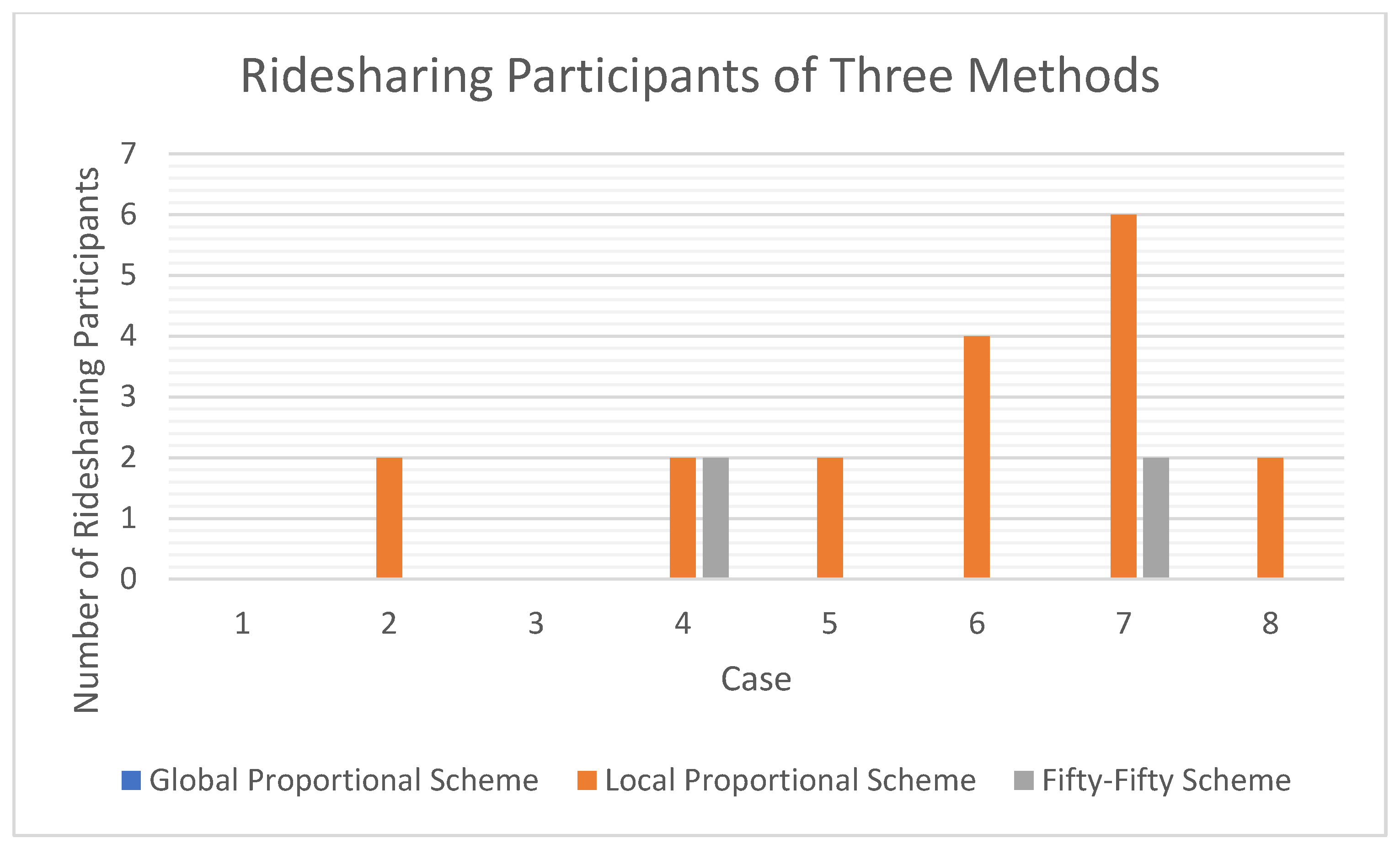
Figure 3 shows the results of the total acceptable rides of Table 11, Table 12, Table 13, Table 14, Table 15, Table 16, Table 17 and Table 18 in bar charts for the three schemes under = 0.2. It is obvious that Property 2 and Property 4 hold. Figure 4 shows the results of the total ridesharing participants of Table 11, Table 12, Table 13, Table 14, Table 15, Table 16, Table 17 and Table 18 in bar charts for the three schemes under = 0.2. It is obvious that Property 1 and Property 3 hold.
Although the results above indicate that there is no “one-size-fits-all” cost savings allocation method suitable for all circumstances, it can be observed that if greedy ridesharing information providers and users have higher expectations of cost savings, the Local Proportional Method is a better choice. If ridesharing information providers and users are generous and have lower expectations of cost savings, the Global Proportional Method is a good choice.
5. Discussion
Two series of experiments were performed based on eight cases to verify the properties characterized in this paper. The properties characterize conditions under which one allocation method performs better or at least the same as another method. The first series of experiments was based on a lower share value for the information provider and a lower minimal expected rewarding rate for drivers. The second series of experiments were based on a higher share value for the information provider and a higher minimal expected rewarding rate for the drivers. As all the properties were established based on the assumption that the minimal expected rewarding rate for drivers and that of passengers might not be equal, the minimal expected rewarding rate for drivers and that of passengers were set to be different in the two series of experiments performed in this paper.
The results of the first series of experiments in Table 3, Table 4, Table 5, Table 6, Table 7, Table 8, Table 9 and Table 10 were used to verify Property 1 and Property 3, which characterized the conditions for the Global Proportional Method to perform better or at least the same as the Local Proportional Method and the Fifty-Fifty Method. The results of the first series of experiments indicate that the Global Proportional Method performed better or at least the same as the Local Proportional Method and the Fifty-Fifty Method in the case that the condition of the information provider share value and a minimal expected rewarding rate are lower. In this case, the Global Proportional Method should be used. The results of the second series of experiments in Table 11, Table 12, Table 13, Table 14, Table 15, Table 16, Table 17 and Table 18 were used to verify Property 2 and Property 4, which characterize the conditions for the Local Proportional Method and the Fifty-Fifty Method to perform better or at least the same as the Global Proportional Method. The results of the second series of experiments indicate that the Local Proportional Method and the Fifty-Fifty Method perform better or at least the same as the Global Proportional Method in the case that the information provider share value and the minimal expected rewarding rate are higher. In this case, the Local Proportional Method should be used as the performance of the Fifty-Fifty Method is inferior to that of the Local Proportional Method. In summary, the Global Proportional Method either outperformed or was as good as the other two methods in the first series of experiments but was inferior to or the same as the other two methods in the second series of experiments.
The results indicated that each of the three methods is neither inferior in all cases nor superior in all cases. Among the three methods, there is no one that either wins in all the cases or loses in all the cases. In summary, the best choice depends on the share value for the information provider as well as the minimal expected rewarding rates for drivers and passengers. Determinants that influence acceptability of cost savings allocation methods in ridesharing systems were not well studied in the literature. In this paper, we show that the minimal expected rewarding rate for drivers, the minimal expected rewarding rate for passengers, and the share value for the information provider are three determinants that jointly influence acceptability of cost savings allocation methods in ridesharing systems. How the three determinants influence performance can be characterized by four properties. These new findings pave the way for choosing the right method to allocate cost savings among the stakeholders in ridesharing systems.
6. Conclusions
Transport cost savings due to a reduction in energy consumption is one of the features and benefits that attract drivers and riders to use the ridesharing model. However, the methods to divide cost savings among ridesharing participants have a significant influence on participants’ willingness to adopt the ridesharing transport mode. Improper allocation of transport cost savings in ridesharing systems may disappoint the users as their expectations of minimal rewarding rates are not satisfied. To make as many users as possible adopt the ridesharing model, the comparison of different methods to allocate transport cost savings in the ridesharing model is an interesting and important issue. In this paper, the previous study on the comparison of three methods to divide cost savings among the ridesharing participants was extended. The underlying assumption that the minimal expected rewarding rate for drivers and that of passengers were equal in the previous study has been relaxed in this paper. Based on this premise, several properties to compare the performance of the three methods were characterized.
In this paper, the influence of the three methods to allocate transport cost savings in ridesharing systems under the premise that drivers’ expectations and passengers’ expectations of minimal rewarding rate may be different has been studied. The performance indices used for comparing the three methods to allocate transport cost savings include total passengers on the acceptable rides, total participants on the acceptable rides, and total acceptable rides. Four properties are presented to compare the performance of the three proportional methods in terms of different performance indices. The results of experiments presented in this paper are consistent with the four properties. The results indicate that applying the proportional allocation methods may lead to different numbers of acceptable rides and ridesharing participants for the same cost savings. The share of cost savings allocated to the ridesharing information provider also has a significant influence on the performance of the proportional allocation methods in terms of the numbers of acceptable rides and ridesharing participants. The four properties presented in this paper are useful to characterize the condition to choose a specific proportional method to allocate cost savings to increase its acceptability to users.
This study indicates that there is no “one-size-fits-all” cost savings allocation method suitable for all circumstances. One interesting finding is that, for greedy ridesharing information providers and users that have higher expectations of cost savings, the Local Proportional Method is a better choice. Another interesting finding is that, for generous ridesharing information providers and users that have lower expectations of cost savings, the Global Proportional Method is a good fit. This study is limited to deterministic ridesharing problems in which the requirements of drivers and riders are deterministic. One challenging research direction is to study stochastic ridesharing problems in which the requirements of drivers and riders are specified by stochastic processes. The results of this paper are based on the analysis of three proportional methods. Analysis of non-proportional methods is a challenging problem. Another interesting future research direction is to design and analyze other methods to divide and allocate cost savings in ridesharing systems. The performance indicators used to compare different methods are all directly linked to the number of users accepting the ridesharing systems. These performance indicators include the number of acceptable rides, the number of passengers on the acceptable rides, and the number of participants on the acceptable rides. Consideration of the other performance indicators not included in this paper will be an interesting research issue. In this paper, it is assumed that the minimal expected rewarding rates are given. The issue to determine minimal expected rewarding rates is an interesting research direction.
Funding
This research was supported in part by the National Science and Technology Council, Taiwan, under Grant NSTC 111-2410-H-324-003.
Data Availability Statement
Data available in a publicly accessible repository described in the article.
Conflicts of Interest
The author declares no conflict of interest.
Appendix A
Proof of Lemma 1.
According to the definition of the Local Proportional Method, the share value for a passenger is defined in Equations (5) and (6). The rewarding rate for a winning passenger with = 1 is defined in Equation (A1)
According to the definition of the Local Proportional Method, the share value for a driver is defined in Equations (7) and (8). As there is at most only one winning bid for a driver, let be the winning bid for driver . That is, . The rewarding rate for a driver is defined in Equation (A2)
Hence the rewarding rate for the driver and the passengers on a shared ride is the same.
To prove that the shared ride under the Global Proportional Method is greater than or equal to the shared ride with the lowest rewarding rate under the Local Proportional Method, it is sufficient to prove that the rewarding rate for the driver and the passengers on the shared ride with minimal rewarding rate is less than or equal to that under the Global Proportional Method.
Let the -th bid of driver be the ride with the lowest rewarding rate under the Local Proportional Method for the solution . Then Equations (A3)–(A5) hold:
Therefore, the following inequality Equation (A6) holds:
By dividing the terms on both sides of the above inequality, Equation (A7) holds:
Note that the left-hand side of the inequality Equation (A7) above is equal to Equation (A8):
The term in Equation (A8) above is equal to Equation (A9):
Note that Equation (A9) can be reduced to Equation (A10):
By replacing the term on the left-hand side of the inequality Equation (A7) with the term in Equation (A10), Equation (A11) holds as follows:
The right-hand side of Equation (A11) is the rewarding rate under the Global Proportional Method and the left-hand side of Equation (A11) is the lowest rewarding rate of the shared ride under the Local Proportional Method.
Therefore, the rewarding rate under the Global Proportional Method is greater than or equal to the lowest rewarding rate of the shared ride under the Local Proportional Method. □
Appendix B
Proof of Property 2
. First, (i), (ii) and (iii) below will be proved and then this property will be proved based on (i), (ii), and (iii).
- (i)
- First, it is shown that the highest rewarding rate for shared rides under the Local Proportional Method is greater than that of the Global Proportional Method. Let the winning bid of driver be the shared ride with the highest rewarding rate for shared rides under the Local Proportional Method.
Then .
As ,
It follows that .
By summing up all the terms on the left-hand side and all the terms on the right-hand side of the above inequality , it follows that . By dividing the terms on the left-hand side and all the terms on the right-hand side of the above inequality by ,
It follows that .
As , it follows that The term on the right-hand side of the above inequality can be reduced to Equation (A12) as follows:
Hence .
Therefore, the highest rewarding rate for shared rides under the Local Proportional Method is greater than or equal to that under the Global Proportional Method.
- (ii)
- If the Local Proportional Method is used, the rewarding rate for passenger is , where . The rewarding rate for passenger is . If the Local Proportional Method is used, the rewarding rate for driver is , where .
The rewarding rate for driver is .
For driver to transport the set of passengers in , the following conditions must be satisfied: and .
The set of drivers accepting ridesharing under the Local Proportional Method is defined in Equation (A13)
The set of passengers accepting ridesharing under the Local Proportional Method is defined in Equation (A14)
- (iii)
- In the Global Proportional Method, the rewarding rate for passenger is . The rewarding rate for passenger is = . In the Global Proportional Method, the rewarding rate for driver is . The rewarding rate for driver is . Therefore, the rewarding rate for each passenger and each driver is the same.
The set of drivers accepting ridesharing under the Global Proportional Method is defined in Equation (A15).
The set of passengers accepting ridesharing under the Global Proportional Method is defined in Equation (A16).
As the rewarding rate under the Global Proportional Method is less than , it follows that .
Case 1: If , . In this case, .
In this case, all winning drivers will not accept the rides. In this case, .
Case 2: If , . In this case, .
In this case, all winning passengers will not accept the rides. In this case, .
Based on Case 1 and Case 2, the number of acceptable rides under the Global Proportional Method is . The number of passengers on the acceptable rides under the Global Proportional Method is . The number of ridesharing participants on the acceptable rides under the Global Proportional Method is . In short, the number of acceptable rides under the Global Proportional Method is zero as either all winning drivers or all winning passengers will not accept the rides.
According to (iii), .
According to (ii), the set of drivers accepting ridesharing under the Local Proportional Method is and the set of passengers accepting ridesharing under Local Proportional Method is .
According to (i), the highest rewarding rate for shared rides under the Local Proportional Method is greater than or equal to that under the Global Proportional Method.
Therefore, and .
The number of acceptable shared rides under the Local Proportional Method is .
The number of passengers on the acceptable shared rides under the Local Proportional Method is .
Therefore, the number of participants on the acceptable rides under the Local Proportional Method is .
This completes the proof. □
Appendix C
Proof of Property 4
. First, (i), (ii), and (iii) below will be proved. Then this property will be proved based on (i), (ii), and (iii).
Let be a solution to the ridesharing problem.
- (i)
- If the Fifty-Fifty Method is used, the rewarding rate for passenger is with .
The rewarding rate for passenger is .
If the Fifty-Fifty Method is used, the rewarding rate for driver is .
The rewarding rate for driver is .
For driver to transport the set of passengers in , the following conditions must be satisfied: and . The set of drivers accepting ridesharing under the Fifty-Fifty Method is . The number of ridesharing drivers under the Fifty-Fifty Method is . The number of acceptable shared rides under the Fifty-Fifty Method is . The set of passengers accepting ridesharing under the Fifty-Fifty Method is . The number of passengers on the acceptable rides under the Fifty-Fifty Method is . The number of ridesharing participants on the acceptable rides under the Fifty-Fifty Method is .
- (ii)
- In the Global Proportional Method, the rewarding rate for passenger is .
The rewarding rate for passenger is = .
In the Global Proportional Method, the rewarding rate for driver is . The rewarding rate for driver is .
Therefore, the rewarding rate for each passenger and each driver is the same.
The set of drivers accepting ridesharing under the Global Proportional Method is
The set of passengers accepting ridesharing under the Global Proportional Method is
As the rewarding rate under the Global Proportional Method is less than , . There are two cases.
Case 1: If , . In this case, the following holds .
In this case, all winning drivers will not accept the rides. In this case, .
Case 2: If , . In this case, the following holds. .
In this case, all winning passengers will not accept the rides. In this case, .
Based on Case 1 and Case 2, the number of acceptable rides under the Global Proportional Method is .
The number of passengers on the acceptable rides under the Global Proportional Method is .
The number of ridesharing participants on the acceptable rides under the Global Proportional Method is . In short, the number of acceptable rides under the Global Proportional Method is zero as either all winning drivers or all winning passengers will not accept the rides.
- (iii)
- According to (i), the number of acceptable shared rides under the Fifty-Fifty Method is .
According to (ii), the number of acceptable rides under the Global Proportional Method is zero.
Therefore, if the rewarding rate is less than under the Global Proportional Method, the number of acceptable shared rides under the Fifty-Fifty Method is greater than or equal to that under the Global Proportional Method.
According to (i), the number of passengers on the acceptable rides under the Fifty-Fifty Method is .
According to (ii), the number of passengers on acceptable rides under the Global Proportional Method is zero. Therefore, if the rewarding rate is less than under the Global Proportional Method, the number of passengers on acceptable rides under the Fifty-Fifty Method is greater than or equal to that under the Global Proportional Method.
According to (i), the number of ridesharing participants on the acceptable rides under the Fifty-Fifty Method is . According to (ii), the number of passengers on acceptable rides under the Global Proportional Method is zero. Therefore, if the rewarding rate is less than under the Global Proportional Scheme, the number of ridesharing participants on acceptable rides under the Fifty-Fifty Scheme is greater than or equal to that under the Global Proportional Method.
This completes the proof. □
References
- International Energy Agency. World Energy Outlook 2018; IEA: Paris, France, 2018; Available online: https://www.iea.org/reports/world-energy-outlook-2018 (accessed on 5 February 2023).
- International Energy Agency. World Energy Outlook 2022; IEA: Paris, France, 2022; Available online: https://www.iea.org/reports/world-energy-outlook-2022 (accessed on 5 February 2023).
- U.S. Energy Information Administration, Monthly Energy Review. 2022. Available online: https://www.eia.gov/totalenergy/data/monthly/archive/00352204.pdf (accessed on 28 February 2023).
- Opstal, W.V.; Borms, L. Startups and circular economy strategies: Profile differences, barriers and enablers. J. Clean. Prod. 2023, 396, 136510. [Google Scholar] [CrossRef]
- Hossain, M. Sharing economy: A comprehensive literature review. Int. J. Hosp. Manag. 2020, 87, 102470. [Google Scholar] [CrossRef]
- Xu, X.; Hao, J.; Zheng, Y. Multi-objective artificial bee colony algorithm for multi-stage resource leveling problem in sharing logistics network. Comput. Ind. Eng. 2020, 142, 106338. [Google Scholar] [CrossRef]
- Vandycke, N.; Sehmi, G.S.; Sandoval, I.R.; Lee, Y. Defining the Role of Transport in the Circular Economy. 2022. Available online: https://blogs.worldbank.org/transport/defining-role-transport-circular-economy (accessed on 5 February 2023).
- Castellanos, S.; Grant-Muller, S.; Wright, K. Technology, transport, and the sharing economy: Towards a working taxonomy for shared mobility. Transp. Rev. 2022, 42, 318–336. [Google Scholar] [CrossRef]
- Mourad, A.; Puchinger, J.; Chu, C. A survey of models and algorithms for optimizing shared mobility. Transp. Res. Part B Methodol. 2019, 123, 323–346. [Google Scholar] [CrossRef]
- Sun, R.; Wu, X.; Chen, Y. Assessing the impacts of ridesharing services: An agent-based simulation approach. J. Clean. Prod. 2022, 372, 133664. [Google Scholar] [CrossRef]
- Li, X.; Xu, J.; Du, M.; Liu, D.; Kwan, M.-P. Understanding the spatiotemporal variation of ride-hailing orders under different travel distances. Travel Behav. Soc. 2023, 32, 100581. [Google Scholar] [CrossRef]
- Wieding, S.V.; Sprei, F.; Hult, C.; Hult, Å.; Roth, A.; Persson, M. Drivers and barriers to business-to-business carsharing for work trips—A case study of Gothenburg, Sweden. Case Stud. Transp. Policy 2022, 10, 2330–2336. [Google Scholar] [CrossRef]
- Bruglieri, M.; Ciccarelli, D.; Colorni, A.; Luè, A. PoliUniPool: A carpooling system for universities. Procedia Soc. Behav. Sci. 2011, 20, 558–567. [Google Scholar] [CrossRef] [Green Version]
- Liftango. Available online: https://www.newcastle.edu.au/our-uni/campuses-and-locations/transport/rideshare-liftango (accessed on 5 February 2023).
- Furuhata, M.; Dessouky, M.; Ordóñez, F.; Brunet, M.; Wang, X.; Koenig, S. Ridesharing: The state-of-the-art and future direc-tions. Transp. Res. Pt. B Methodol. 2013, 57, 28–46. [Google Scholar] [CrossRef]
- Agatz, N.; Erera, A.; Savelsbergh, M.; Wang, X. Optimization for dynamic ride-sharing: A review. Eur. J. Oper. Res. 2012, 223, 295–303. [Google Scholar] [CrossRef]
- Brown, A.E. Who and where rideshares? Rideshare travel and use in Los Angeles. Transp. Res. Part A Policy Pract. 2020, 136, 120–134. [Google Scholar] [CrossRef]
- Hwang, K.; Giuliano, G. The Determinants of Ridesharing: Literature Review; Working Paper UCTC No. 38; The University of California Transportation Center: Berkeley, CA, USA, 1990; Available online: https://escholarship.org/uc/item/3r91r3r4 (accessed on 5 February 2023).
- Zhang, F.; Roberts, S.; Goldman, C. A Survey Study Measuring People’s Preferences Towards Automated and Non-Automated Ridesplitting. In Proceedings of the Driving Assessment Conference 10, Santa Fe, NM, USA, 24–27 June 2019; pp. 92–98. [Google Scholar]
- Thaithatkul, P.; Seo, T.; Kusakabe, T.; Asakura, Y. Adoption of dynamic ridesharing system under influence of information on social network. Transp. Res. Procedia 2019, 37, 401–408. [Google Scholar] [CrossRef]
- Hsieh, F.-S. Development and Comparison of Ten Differential-Evolution and Particle Swarm-Optimization Based Algorithms for Discount-Guaranteed Ridesharing Systems. Appl. Sci. 2022, 12, 9544. [Google Scholar] [CrossRef]
- Hsieh, F.-S. Grouping Patients for Ridesharing in Non-emergency Medical Care Services, To appear. In Proceedings of the 13th IEEE Annual Computing and Communication Workshop and Conference (CCWC 2023), Virtual, 8–11 March 2023; pp. 939–942. [Google Scholar]
- Hsieh, F.S. A Comparative Study of Several Metaheuristic Algorithms to Optimize Monetary Incentive in Ridesharing Systems. ISPRS Int. J. Geo-Inf. 2020, 9, 590. [Google Scholar] [CrossRef]
- Berlingerio, M.; Ghaddar, B.; Guidotti, R.; Pascale, A.; Sassi, A. The GRAAL of carpooling: GReen And sociAL optimization from crowd-sourced data. Transp. Res. Part C Emerg. Technol. 2017, 80, 20–36. [Google Scholar] [CrossRef]
- Saisubramanian, S.; Basich, C.; Zilberstein, S.; Goldman, C.V. Satisfying Social Preferences in Ridesharing Services. In Proceedings of the 2019 IEEE Intelligent Transportation Systems Conference (ITSC), Auckland, New Zealand, 27–30 October 2019; pp. 3720–3725. [Google Scholar]
- Hsieh, F.S. Trust-Based Recommendation for Shared Mobility Systems Based on a Discrete Self-Adaptive Neighborhood Search Differential Evolution Algorithm. Electronics 2022, 11, 776. [Google Scholar] [CrossRef]
- Bistaffa, F.; Farinelli, A.; Ramchurn, S.D. Sharing rides with friends: A coalition formation algorithm for ridesharing. In Proceedings of the 29th AAAI Conference on Artificial Intelligence, Austin, TX, USA, 25–30 January 2015; pp. 608–614. [Google Scholar]
- Sun, Z.; Wang, Y.; Zhou, H.; Jiao, J.; Overstreet, R.E. Travel behaviours, user characteristics, and social-economic impacts of shared transportation: A comprehensive review. Int. J. Logist. Res. Appl. 2021, 24, 51–78. [Google Scholar] [CrossRef]
- Hyland, M.; Mahmassani, H.S. Operational benefits and challenges of shared-ride automated mobility-on-demand services. Transp. Res. Part A Policy Pract. 2020, 134, 251–270. [Google Scholar] [CrossRef]
- Hansen, T.; Sener, I.N. Strangers on this Road We Are on: A Literature Review of Pooling in on-Demand Mobility Services. Transp. Res. Rec. 2022. [Google Scholar] [CrossRef]
- Waerden, P.; Lem, A.; Schaefer, W. Investigation of Factors that Stimulate Car Drivers to Change from Car to Carpooling in City Center Oriented Work Trips. Transp. Res. Procedia 2015, 10, 335–344. [Google Scholar] [CrossRef] [Green Version]
- Guajardoa, M.; Ronnqvist, M. A review on cost allocation methods in collaborative transportation. Int. Trans. Oper. Res. 2016, 23, 371–392. [Google Scholar] [CrossRef]
- Kalai, E. Proportional solutions to bargaining situations: Intertemporal utility comparisons. Econometrica 1977, 45, 1623–1630. [Google Scholar] [CrossRef]
- Schmeidler, D. The Nucleolus of a Characteristic Function Game. SIAM J. Appl. Math. 1969, 17, 1163–1170. [Google Scholar] [CrossRef]
- Shapley, L.S. A Value for N-Person Games. A Value N-Pers. Games 1952, 28, 307–317. [Google Scholar]
- Perea, F.; Puerto, J. A heuristic procedure for computing the nucleolus. Comput. Oper. Res. 2019, 112, 104764. [Google Scholar] [CrossRef]
- Fatima, S.S.; Wooldridge, M.; Jennings, N.R. A linear approximation method for the Shapley value. Artif. Intell. 2008, 172, 1673–1699. [Google Scholar] [CrossRef] [Green Version]
- Levinger, C.; Hazon, N.; Azaria, A. Computing the Shapley Value for Ride-Sharing and Routing Games. In Proceedings of the 19th International Conference on Autonomous Agents and Multi-Agent Systems, Auckland, New Zealand, 9–13 May 2020; pp. 1895–1897. [Google Scholar]
- Lu, W.; Quadrifoglio, L. Fair cost allocation for ridesharing services—Modeling, mathematical programming and an algorithm to find the nucleolus. Transp. Res. Part B Methodol. 2019, 121, 41–55. [Google Scholar] [CrossRef] [Green Version]
- Cipolina-Kun, L.; Yazdanpanah, V.; Stein, S.; Gerding, E.H. A Proportional Pricing Mechanism for Ridesharing Services with Meeting Points. In Proceedings of the PRIMA 2022: Principles and Practice of Multi-Agent Systems: 24th International Conference, Valencia, Spain, 16–18 November 2022; pp. 523–539. [Google Scholar]
- Wang, X.; Agatz, N.; Erera, A. Stable Matching for Dynamic Ride-Sharing Systems. Transp. Sci. 2018, 52, 850–867. [Google Scholar] [CrossRef]
- Agatz, N.A.H.; Erera, A.L.; Savelsbergh, M.W.P.; Wang, X. Dynamic ride-sharing: A simulation study in metro Atlanta. Transp. Res. Part B Methodol. 2011, 45, 1450–1464. [Google Scholar] [CrossRef]
- Hsieh, F.S.; Zhan, F.; Guo, Y. A solution methodology for carpooling systems based on double auctions and cooperative coevolutionary particle swarms. Appl. Intell. 2019, 49, 741–763. [Google Scholar] [CrossRef]
- Hsieh, F.-S. A Comparison of Three Ridesharing Cost Savings Allocation Schemes Based on the Number of Acceptable Shared Rides. Energies 2021, 14, 6931. [Google Scholar] [CrossRef]
Figure 1.
Verification of Property 1 and Property 3 for total acceptable rides of Case 1 through Case 8 under = 0.05.
Figure 1.
Verification of Property 1 and Property 3 for total acceptable rides of Case 1 through Case 8 under = 0.05.

Figure 2.
Verification of Property 1 and Property 3 for total ridesharing participants of three schemes for Case 1 through Case 8 under = 0.05.
Figure 2.
Verification of Property 1 and Property 3 for total ridesharing participants of three schemes for Case 1 through Case 8 under = 0.05.
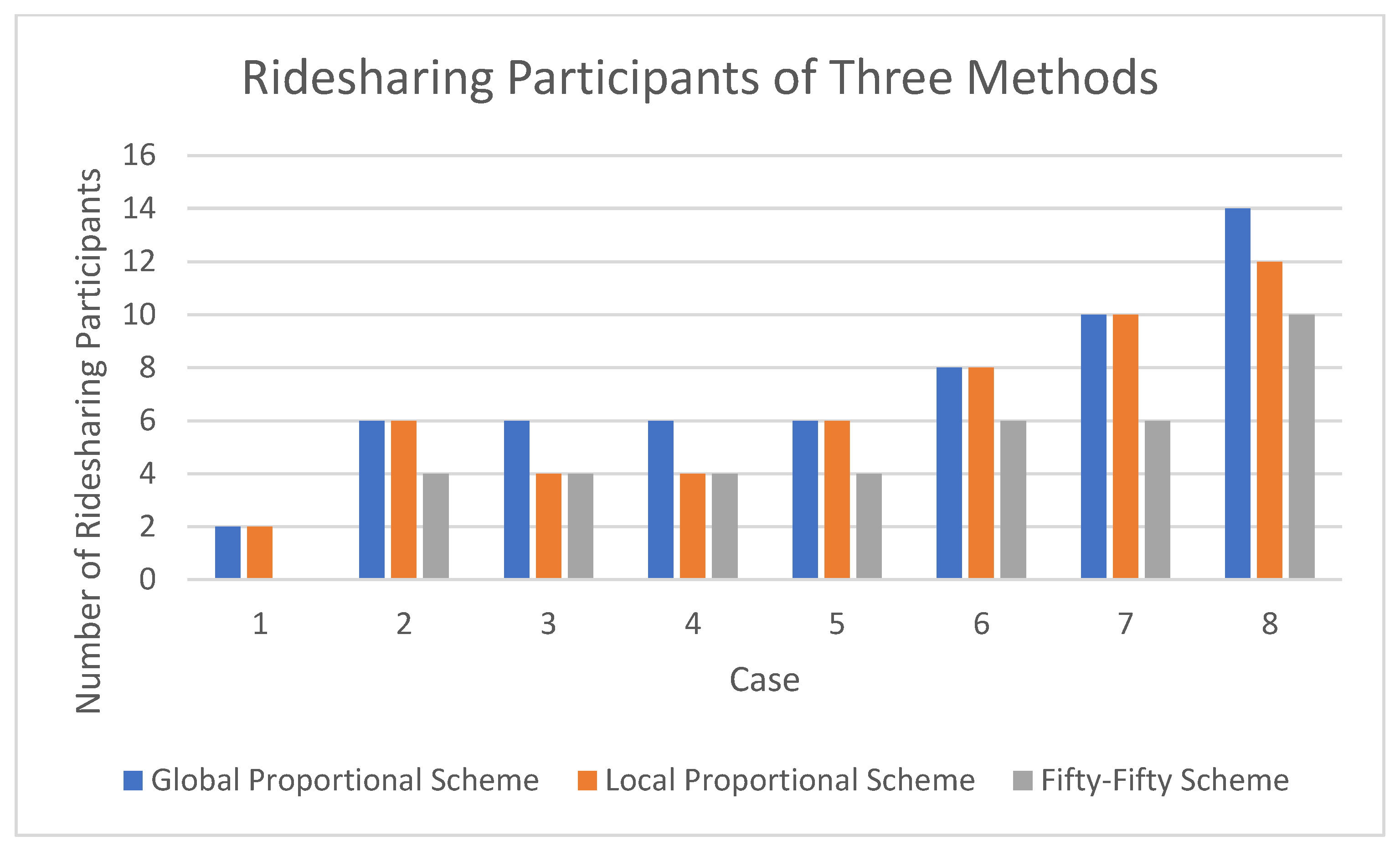
Figure 3.
Verification of Property 2 and Property 4 for total acceptable rides of three schemes under = 0.2.
Figure 3.
Verification of Property 2 and Property 4 for total acceptable rides of three schemes under = 0.2.
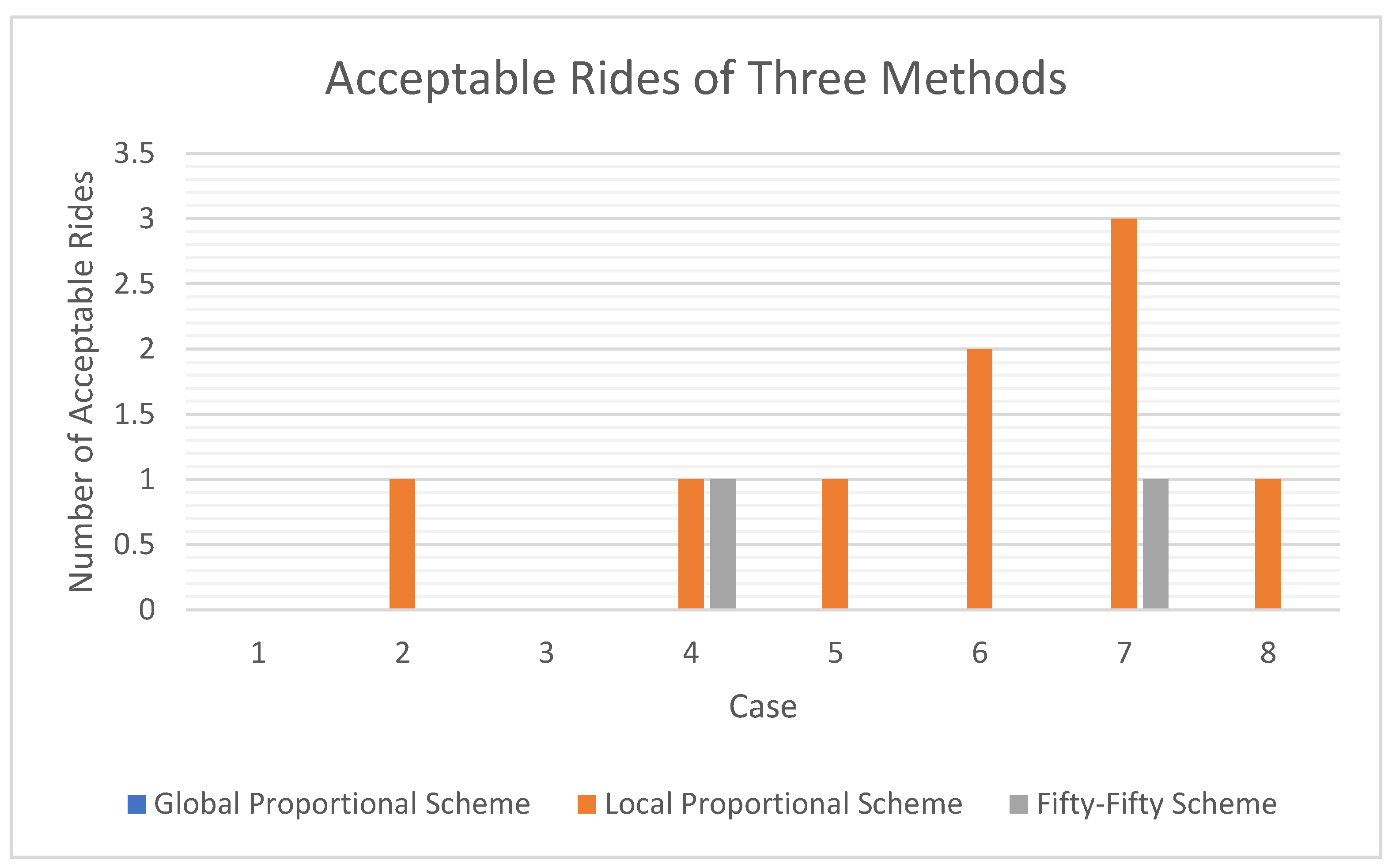
Figure 4.
Verification of Property 2 and Property 4 for total acceptable rides of three schemes under = 0.2.
Figure 4.
Verification of Property 2 and Property 4 for total acceptable rides of three schemes under = 0.2.

Table 1.
Notations of symbols, variables, and parameters.
| Variable | Meaning |
|---|---|
| a passenger, and is the number of passengers | |
| a driver, and is the number of drivers | |
| the index of a location, | |
| total bids submitted by driver | |
| A bid of a driver, and is the number of bids submitted by driver driver ‘s -th bid | |
| = , where : seats allocated to pick-up location of passenger , : seats released at drop-off location of passenger , : original cost of the driver without ridesharing : the transport cost of driver ’s -th bid. | |
| passenger ’s bid = , where : seats requested for pick-up location of passenger , : seats released at drop-off location of passenger , : passenger ’s original cost without ridesharing. | |
| driver ’s decision variable; if = 1, the bid of driver is a winning bid and the bid of driver is not a winning bid otherwise ( = 0) | |
| passenger ’s decision variable; if = 1, passenger ’s bid is a winning bid and passenger ’s bid is not a winning bid otherwise ( = 0) | |
| ridesharing information provider’s share value | |
| passenger ’s share value | |
| driver ’s share value | |
| the set of passengers on the ride of driver ’s –th bid | |
| the cost savings function | |
| the cost savings function of driver ’s –th bid |
Table 2.
Three methods to divide savings of cost among the ridesharing participants.
| Scheme | Stakeholder | Share Value | |
|---|---|---|---|
| Fifty-Fifty (FF) Method | information provider | (7) | |
| passenger | (8) | ||
| driver | (9) | ||
| Local Proportional (LP) Method | information provider | (10) | |
| passenger | (11) | ||
| where, | (12) | ||
| driver | (13) | ||
| where, | (14) | ||
| Global Proportional (GP) Method | information provider | (15) | |
| passenger | (16) | ||
| driver | (17) |
Table 3.
Number of drivers and passengers accepted in Case 1 for = 0.05, = 0.11 and = 0.1.
| Case 1 | Participant | GP | GP Accepted | LP | LP Accepted | FF | FF Accepted |
|---|---|---|---|---|---|---|---|
| Ride 1 | D1 | 0.114 | 1 | 0.114 | 1 | 0.069 | 0 |
| P1 | 0.114 | 1 | 0.114 | 1 | 0.34 | 0 | |
| Total rides | 1 | 1 | 0 | ||||
| Participants on acceptable rides | 2 | 2 | 0 |
Table 4.
Number of drivers and passengers accepted in Case 2 for = 0.05, = 0.11 and = 0.1.
| Case 2 | Participant | GP | GP Accepted | LP | LP Accepted | FF | FF Accepted |
|---|---|---|---|---|---|---|---|
| Ride 1 | D1 | 0.21 | 1 | 0.119 | 1 | 0.068 | 0 |
| P1 | 0.21 | 1 | 0.119 | 1 | 0.475 | 0 | |
| Ride 2 | D2 | 0.21 | 1 | 0.218 | 1 | 0.142 | 1 |
| P2 | 0.21 | 1 | 0.218 | 1 | 0.475 | 1 | |
| Ride 3 | D3 | 0.21 | 1 | 0.277 | 1 | 0.196 | 1 |
| P3 | 0.21 | 1 | 0.277 | 1 | 0.475 | 1 | |
| Total rides | 3 | 3 | 2 | ||||
| Participants on acceptable rides | 6 | 6 | 4 |
Table 5.
Number of drivers and passengers accepted in Case 3 for = 0.05, = 0.11 and = 0.1.
| Case 3 | Participant | GP | GP Accepted | LP | LP Accepted | FF | FF Accepted |
|---|---|---|---|---|---|---|---|
| Ride 1 | D1 | 0.166 | 1 | 0.189 | 1 | 0.121 | 1 |
| P1 | 0.166 | 1 | 0.189 | 1 | 0.438 | 1 | |
| Ride 2 | D2 | 0.166 | 1 | 0.098 | 0 | 0.06 | 0 |
| P2 | 0.166 | 1 | 0.098 | 0 | 0.258 | 0 | |
| Ride 3 | D3 | 0.166 | 1 | 0.193 | 1 | 0.121 | 1 |
| P3 | 0.166 | 1 | 0.193 | 1 | 0.475 | 1 | |
| Total rides | 3 | 2 | 2 | ||||
| Participants on acceptable rides | 6 | 4 | 4 |
Table 6.
Number of drivers and passengers accepted in Case 4 for = 0.05, = 0.11 and = 0.1.
| Case 4 | Participant | GP | GP Accepted | LP | LP Accepted | FF | FF Accepted |
|---|---|---|---|---|---|---|---|
| Ride 1 | D1 | 0.209 | 1 | 0.232 | 1 | 0.154 | 1 |
| P1 | 0.209 | 1 | 0.232 | 1 | 0.475 | 1 | |
| Ride 2 | D2 | 0.209 | 1 | 0.054 | 0 | 0.034 | 0 |
| P2 | 0.209 | 1 | 0.054 | 0 | 0.132 | 0 | |
| Ride 3 | D3 | 0.209 | 1 | 0.353 | 1 | 0.28 | 1 |
| P3 | 0.209 | 1 | 0.353 | 1 | 0.475 | 1 | |
| Total rides | 3 | 2 | 2 | ||||
| Participants on acceptable rides | 6 | 4 | 4 |
Table 7.
Number of drivers and passengers accepted in Case 5 for = 0.05, = 0.12 and = 0.1.
| Case 5 | Participant | GP | GP Accepted | LP | LP Accepted | FF | FF Accepted |
|---|---|---|---|---|---|---|---|
| Ride 1 | D1 | 0.207 | 1 | 0.265 | 1 | 0.184 | 1 |
| P1 | 0.207 | 1 | 0.265 | 1 | 0.475 | 1 | |
| Ride 2 | D2 | 0.207 | 1 | 0.138 | 1 | 0.081 | 0 |
| P2 | 0.207 | 1 | 0.138 | 1 | 0.475 | 0 | |
| Ride 3 | D3 | 0.207 | 1 | 0.223 | 1 | 0.145 | 1 |
| P3 | 0.207 | 1 | 0.223 | 1 | 0.475 | 1 | |
| Total rides | 3 | 3 | 2 | ||||
| Participants on acceptable rides | 6 | 6 | 4 |
Table 8.
Number of drivers and passengers accepted in Case 6 for = 0.05, = 0.11 and = 0.1.
| Case 6 | Participant | GP | GP Accepted | LP | LP Accepted | FF | FF Accepted |
|---|---|---|---|---|---|---|---|
| Ride 1 | D1 | 0.2 | 1 | 0.192 | 1 | 0.123 | 1 |
| P1 | 0.2 | 1 | 0.192 | 1 | 0.434 | 1 | |
| Ride 2 | D2 | 0.2 | 1 | 0.12 | 1 | 0.069 | 0 |
| P2 | 0.2 | 1 | 0.12 | 1 | 0.471 | 0 | |
| Ride 3 | D3 | 0.2 | 1 | 0.253 | 1 | 0.172 | 1 |
| P3 | 0.2 | 1 | 0.253 | 1 | 0.475 | 1 | |
| Ride 4 | D4 | 0.2 | 1 | 0.254 | 1 | 0.174 | 1 |
| P4 | 0.2 | 1 | 0.254 | 1 | 0.475 | 1 | |
| Total rides | 4 | 4 | 3 | ||||
| Participants on acceptable rides | 8 | 8 | 6 |
Table 9.
Number of drivers and passengers accepted in Case 7 for = 0.05, = 0.11 and = 0.1.
| Case 7 | Participant | GP | GP Accepted | LP | LP Accepted | FF | FF Accepted |
|---|---|---|---|---|---|---|---|
| Ride 1 | D1 | 0.234 | 1 | 0.241 | 1 | 0.172 | 1 |
| P1 | 0.234 | 1 | 0.241 | 1 | 0.401 | 1 | |
| Ride 2 | D2 | 0.234 | 1 | 0.238 | 1 | 0.159 | 1 |
| P2 | 0.234 | 1 | 0.238 | 1 | 0.475 | 1 | |
| Ride 3 | D3 | 0.234 | 1 | 0.144 | 1 | 0.085 | 0 |
| P3 | 0.234 | 1 | 0.144 | 1 | 0.475 | 0 | |
| Ride 4 | D4 | 0.234 | 1 | 0.153 | 1 | 0.091 | 0 |
| P4 | 0.234 | 1 | 0.153 | 1 | 0.475 | 0 | |
| Ride 5 | D5 | 0.234 | 1 | 0.331 | 1 | 0.254 | 1 |
| P5 | 0.234 | 1 | 0.331 | 1 | 0.475 | 1 | |
| Total rides | 5 | 5 | 3 | ||||
| Participants on acceptable rides | 10 | 10 | 6 |
Table 10.
Number of drivers and passengers accepted in Case 8 for = 0.05, = 0.11 and = 0.1.
| Case 8 | Participant | GP | GP Accepted | LP | LP Accepted | FF | FF Accepted |
|---|---|---|---|---|---|---|---|
| Ride 1 | D1 | 0.181 | 1 | 0.222 | 1 | 0.155 | 1 |
| P1 | 0.181 | 1 | 0.222 | 1 | 0.389 | 1 | |
| Ride 2 | D2 | 0.181 | 1 | 0.223 | 1 | 0.146 | 1 |
| P2 | 0.181 | 1 | 0.223 | 1 | 0.475 | 1 | |
| Ride 3 | D3 | 0.181 | 1 | 0.275 | 1 | 0.194 | 1 |
| P3 | 0.181 | 1 | 0.275 | 1 | 0.475 | 1 | |
| Ride 4 | D4 | 0.181 | 1 | 0.21 | 1 | 0.135 | 1 |
| P4 | 0.181 | 1 | 0.21 | 1 | 0.475 | 1 | |
| Ride 5 | D5 | 0.181 | 1 | 0.145 | 1 | 0.085 | 0 |
| P5 | 0.181 | 1 | 0.145 | 1 | 0.475 | 0 | |
| Ride 6 | D6 | 0.181 | 1 | 0.029 | 0 | 0.019 | 0 |
| P6 | 0.181 | 1 | 0.029 | 0 | 0.062 | 0 | |
| Ride 7 | D7 | 0.181 | 1 | 0.2 | 1 | 0.127 | 1 |
| P7 | 0.181 | 1 | 0.2 | 1 | 0.475 | 1 | |
| Total rides | 7 | 6 | 5 | ||||
| Participants on acceptable rides | 14 | 12 | 10 |
Table 11.
Number of drivers and passengers accepted in Case 1 for = 0.2, = 0.2 and = 0.1.
| Case 1 | Participant | GP | GP Accepted | LP | LP Accepted | FF | FF Accepted |
|---|---|---|---|---|---|---|---|
| Ride 1 | D1 | 0.096 | 0 | 0.096 | 0 | 0.058 | 0 |
| P1 | 0.096 | 0 | 0.096 | 0 | 0.286 | 0 | |
| Total rides | 0 | 0 | 0 | ||||
| Participants on acceptable rides | 0 | 0 | 0 |
Table 12.
Number of drivers and passengers accepted in Case 2 for = 0.2, = 0.2 and = 0.1.
| Case 2 | Participant | GP | GP Accepted | LP | LP Accepted | FF | FF Accepted |
|---|---|---|---|---|---|---|---|
| Ride 1 | D1 | 0.176 | 0 | 0.1 | 0 | 0.057 | 0 |
| P1 | 0.176 | 0 | 0.1 | 0 | 0.4 | 0 | |
| Ride 2 | D2 | 0.176 | 0 | 0.184 | 0 | 0.119 | 0 |
| P2 | 0.176 | 0 | 0.184 | 0 | 0.4 | 0 | |
| Ride 3 | D3 | 0.176 | 0 | 0.234 | 1 | 0.165 | 0 |
| P3 | 0.176 | 0 | 0.234 | 1 | 0.4 | 0 | |
| Total rides | 0 | 1 | 0 | ||||
| Participants on acceptable rides | 0 | 2 | 0 |
Table 13.
Number of drivers and passengers accepted in Case 3 for = 0.2, = 0.2 and = 0.1.
| Case 3 | Participant | GP | GP Accepted | LP | LP Accepted | FF | FF Accepted |
|---|---|---|---|---|---|---|---|
| Ride 1 | D1 | 0.14 | 0 | 0.159 | 0 | 0.102 | 0 |
| P1 | 0.14 | 0 | 0.159 | 0 | 0.369 | 0 | |
| Ride 2 | D2 | 0.14 | 0 | 0.082 | 0 | 0.051 | 0 |
| P2 | 0.14 | 0 | 0.082 | 0 | 0.217 | 0 | |
| Ride 3 | D3 | 0.14 | 0 | 0.163 | 0 | 0.102 | 0 |
| P3 | 0.14 | 0 | 0.163 | 0 | 0.4 | 0 | |
| Total rides | 0 | 0 | 0 | ||||
| Participants on acceptable rides | 0 | 0 | 0 |
Table 14.
Number of drivers and passengers accepted in Case 4 for = 0.2, = 0.2 and = 0.1.
| Case 4 | Participant | GP | GP Accepted | LP | LP Accepted | FF | FF Accepted |
|---|---|---|---|---|---|---|---|
| Ride 1 | D1 | 0.176 | 0 | 0.196 | 0 | 0.13 | 0 |
| P1 | 0.176 | 0 | 0.196 | 0 | 0.4 | 0 | |
| Ride 2 | D2 | 0.176 | 0 | 0.045 | 0 | 0.029 | 0 |
| P2 | 0.176 | 0 | 0.045 | 0 | 0.111 | 0 | |
| Ride 3 | D3 | 0.176 | 0 | 0.297 | 1 | 0.236 | 1 |
| P3 | 0.176 | 0 | 0.297 | 1 | 0.4 | 1 | |
| Total rides | 0 | 1 | 1 | ||||
| Participants on acceptable rides | 0 | 2 | 2 |
Table 15.
Number of drivers and passengers accepted in Case 5 for = 0.2, = 0.2 and = 0.1.
| Case 5 | Participant | GP | GP Accepted | LP | LP Accepted | FF | FF Accepted |
|---|---|---|---|---|---|---|---|
| Ride 1 | D1 | 0.174 | 0 | 0.224 | 1 | 0.155 | 0 |
| P1 | 0.174 | 0 | 0.224 | 1 | 0.4 | 0 | |
| Ride 2 | D2 | 0.174 | 0 | 0.116 | 0 | 0.068 | 0 |
| P2 | 0.174 | 0 | 0.116 | 0 | 0.4 | 0 | |
| Ride 3 | D3 | 0.174 | 0 | 0.187 | 0 | 0.122 | 0 |
| P3 | 0.174 | 0 | 0.187 | 0 | 0.4 | 0 | |
| Total rides | 0 | 1 | 0 | ||||
| Participants on acceptable rides | 0 | 2 | 0 |
Table 16.
Number of drivers and passengers accepted in Case 6 for = 0.2, = 0.2 and = 0.1.
| Case 6 | Participant | GP | GP Accepted | LP | LP Accepted | FF | FF Accepted |
|---|---|---|---|---|---|---|---|
| Ride 1 | D1 | 0.168 | 0 | 0.161 | 0 | 0.103 | 0 |
| P1 | 0.168 | 0 | 0.161 | 0 | 0.365 | 0 | |
| Ride 2 | D2 | 0.168 | 0 | 0.101 | 0 | 0.058 | 0 |
| P2 | 0.168 | 0 | 0.101 | 0 | 0.397 | 0 | |
| Ride 3 | D3 | 0.168 | 0 | 0.213 | 1 | 0.145 | 0 |
| P3 | 0.168 | 0 | 0.213 | 1 | 0.4 | 0 | |
| Ride 4 | D4 | 0.168 | 0 | 0.214 | 1 | 0.146 | 0 |
| P4 | 0.168 | 0 | 0.214 | 1 | 0.4 | 0 | |
| Total rides | 0 | 2 | 0 | ||||
| Participants on acceptable rides | 0 | 4 | 0 |
Table 17.
Number of drivers and passengers accepted in Case 7 for = 0.2, = 0.2 and = 0.1.
| Case 7 | Participant | GP | GP Accepted | LP | LP Accepted | FF | FF Accepted |
|---|---|---|---|---|---|---|---|
| Ride 1 | D1 | 0.197 | 0 | 0.203 | 1 | 0.145 | 0 |
| P1 | 0.197 | 0 | 0.203 | 1 | 0.337 | 0 | |
| Ride 2 | D2 | 0.197 | 0 | 0.201 | 1 | 0.134 | 0 |
| P2 | 0.197 | 0 | 0.201 | 1 | 0.4 | 0 | |
| Ride 3 | D3 | 0.197 | 0 | 0.121 | 0 | 0.071 | 0 |
| P3 | 0.197 | 0 | 0.121 | 0 | 0.4 | 0 | |
| Ride 4 | D4 | 0.197 | 0 | 0.129 | 0 | 0.077 | 0 |
| P4 | 0.197 | 0 | 0.129 | 0 | 0.4 | 0 | |
| Ride 5 | D5 | 0.197 | 0 | 0.279 | 1 | 0.214 | 1 |
| P5 | 0.197 | 0 | 0.279 | 1 | 0.4 | 1 | |
| Total rides | 0 | 3 | 1 | ||||
| Participants on acceptable rides | 0 | 6 | 2 |
Table 18.
Number of drivers and passengers accepted in Case 8 for = 0.2, = 0.2 and = 0.1.
| Case 8 | Participant | GP | GP Accepted | LP | LP Accepted | FF | FF Accepted |
|---|---|---|---|---|---|---|---|
| Ride 1 | D1 | 0.152 | 0 | 0.187 | 0 | 0.131 | 0 |
| P1 | 0.152 | 0 | 0.187 | 0 | 0.328 | 0 | |
| Ride 2 | D2 | 0.152 | 0 | 0.188 | 0 | 0.123 | 0 |
| P2 | 0.152 | 0 | 0.188 | 0 | 0.4 | 0 | |
| Ride 3 | D3 | 0.152 | 0 | 0.232 | 1 | 0.163 | 0 |
| P3 | 0.152 | 0 | 0.232 | 1 | 0.4 | 0 | |
| Ride 4 | D4 | 0.152 | 0 | 0.177 | 0 | 0.114 | 0 |
| P4 | 0.152 | 0 | 0.177 | 0 | 0.4 | 0 | |
| Ride 5 | D5 | 0.152 | 0 | 0.122 | 0 | 0.072 | 0 |
| P5 | 0.152 | 0 | 0.122 | 0 | 0.4 | 0 | |
| Ride 6 | D6 | 0.152 | 0 | 0.025 | 0 | 0.016 | 0 |
| P6 | 0.152 | 0 | 0.025 | 0 | 0.052 | 0 | |
| Ride 7 | D7 | 0.152 | 0 | 0.169 | 0 | 0.107 | 0 |
| P7 | 0.152 | 0 | 0.169 | 0 | 0.4 | 0 | |
| Total rides | 0 | 1 | 0 | ||||
| Participants on acceptable rides | 0 | 2 | 0 |
Disclaimer/Publisher’s Note: The statements, opinions and data contained in all publications are solely those of the individual author(s) and contributor(s) and not of MDPI and/or the editor(s). MDPI and/or the editor(s) disclaim responsibility for any injury to people or property resulting from any ideas, methods, instructions or products referred to in the content. |
© 2023 by the author. Licensee MDPI, Basel, Switzerland. This article is an open access article distributed under the terms and conditions of the Creative Commons Attribution (CC BY) license (https://creativecommons.org/licenses/by/4.0/).
Share and Cite
MDPI and ACS Style
Hsieh, F.-S. Improving Acceptability of Cost Savings Allocation in Ridesharing Systems Based on Analysis of Proportional Methods. Systems 2023, 11, 187. https://doi.org/10.3390/systems11040187
AMA Style
Hsieh F-S. Improving Acceptability of Cost Savings Allocation in Ridesharing Systems Based on Analysis of Proportional Methods. Systems. 2023; 11(4):187. https://doi.org/10.3390/systems11040187
Chicago/Turabian StyleHsieh, Fu-Shiung. 2023. "Improving Acceptability of Cost Savings Allocation in Ridesharing Systems Based on Analysis of Proportional Methods" Systems 11, no. 4: 187. https://doi.org/10.3390/systems11040187
Note that from the first issue of 2016, this journal uses article numbers instead of page numbers. See further details here.