The Climate Change-Road Safety-Economy Nexus: A System Dynamics Approach to Understanding Complex Interdependencies

Abstract

Road accidents have the highest externality costs to society and to the economy, even when compared to the externality damages associated with air emissions and oil dependency. Road safety is one of the most complicated topics, which involves many interdependencies, and so, a sufficiently thorough analysis of roadway safety will require a novel system-based approach in which the associated feedback relationships and causal effects are given appropriate consideration. The factors affecting accident frequency and severity are highly dependent on economic parameters, environmental factors and weather conditions. In this study, we try to use a system dynamics modeling approach to model the climate change-road safety-economy nexus, thereby investigating the complex interactions among these important areas by tracking how they affect each other over time. For this purpose, five sub-models are developed to model each aspect of the overall nexus and to interact with each other to simulate the overall system. As a result, this comprehensive model can provide a platform for policy makers to test the effectiveness of different policy scenarios to reduce the negative consequences of traffic accidents and improve road safety.

1. Introduction

Road accidents are responsible for more than 1.2 million deaths and more than 50 million injuries annually, and so, the need to take very quick and effective actions to reduce road accidents and accident-related fatalities and injuries is inevitable [1]. Based on current trends, it has been predicted that the number of fatalities and injuries from road accidents will become the third leading contributor to the global burden of disease and injuries by 2020 [2,3]. Furthermore, surface transportation (i.e., cars, trucks, etc.) is still the most important sub-sector of transportation for people and commerce in the United States [4], and due to the immense losses in different aspects with respect to the transportation sector (e.g., human, social, environmental and economic aspects), traffic safety has become a major area of concern in the transportation industry [5]. This makes it all the more critical for policy makers to provide a good infrastructure system in order to make surface transportation as safe and efficient as possible, and yet, the currently increasing trends in accident-related fatalities and injuries show that, despite policy makers’ efforts thus far to reduce these fatalities and injuries, society still has a long way to go in order to accomplish the preset goals currently established. In the U.S, despite all efforts to reduce the number of road accidents and accident-related fatalities, the number of annual roadway fatalities has never dropped below 30,000 in the last 50 years [6]. The ultimate goals of transportation safety engineers are to reduce the number of crashes and to mitigate the severity of crash-related injuries [7]. One of the main problems with the complex issues of road safety is the sheer number and variety of the parameters simultaneously playing different roles in traffic accident rates. These parameters frequently tend to affect each other on a short-term or long-term basis, potentially making a bad situation even worse.

As of today, there are different ways to categorize traffic accidents. Some past studies and reports attempted to put more emphasis on the number of vehicles involved in a particular crash, i.e., 1 vehicle crashes, 2 vehicle crashes and 3+-vehicle crashes [8]. Other studies and reports place the main reasons for any crashes under three main categories:

• Driver-related factors, or whether or not the accident in question was the fault of any or all of the driver(s) involved.
• Vehicle-related factors, or whether or not the accident may have been caused by any safety issue(s) with respect to any or all of the vehicle(s) in question and
• Infrastructure/road-related factors, or whether or not improper or damaged infrastructure may have caused the accident.

The main purpose of conventional traffic safety analysis is to find a relationship between the different parameters involved in any given accident, such as driver-related factors, roadway conditions, environmental factors and other such parameters [9]. This paper therefore seeks to develop sub-models capable of investigating each of these three main factors, with the main focus being on driver-related factors, which are the primary category of factors involved in accident rates.

Climate change is another key factor that plays a very important role in accidents and should be seriously investigated as such and considered in long-term road safety planning. As such, environmental factors connected to climate change and the like have become a major obstacle to road transportation safety, especially now that climate change has become one of the most important issues of the 21st century due to recent tremendous environmental changes. These environmental changes have a strong impact on road safety; according to the U.S. Department of Transportation (USDOT), weather-related accidents account for nearly 23% out of almost six million accidents per year. By definition, weather-related crashes are traffic accidents that occur under adverse weather conditions (rain, snow, fog, etc.) or accidents that occur on slick (e.g., wet or slushy) pavement. The negative effects of climate change can be projected as increasing the frequency of extreme weather events, such as heat waves, rising sea levels, storms, hurricanes, floods, etc. [10]. Road transportation safety is compromised under any of these conditions or any possible combination thereof, either due to vehicle safety measures becoming less effective than they might be under normal weather conditions or due to the destructive effects of extreme weather conditions on roads and infrastructures.

For example, extremely hot weather conditions can cause cars to overheat and accelerate tire deterioration and may also soften asphalt, the latter of which can lead to asphalt deformation, thermal expansion of bridge joints and other potential hazards [11]. As another example, rising sea levels (especially for transportation in coastal areas, which are more vulnerable to sea-level rise) may lead to floods that can cause skidding and even drowning of the vehicles and may also cause infrastructure erosion. Ultimately, the main concern regarding all of these sudden unpredictable weather changes is that today’s infrastructure has generally been designed to last for a certain preset period of time, based on predicted weather conditions that can no longer be considered valid due to rapid climate change. As a result, all of the original infrastructure designs must be changed or even discarded altogether, in favor of new designed models based on the changing weather patterns [12].

Numerous studies have investigated the effects of adverse weather conditions on road accidents. In order to classify these effects and their associated consequences, the USDOT has released a report about its road weather management program, in which different weather variables are classified into different groups, including air temperature/humidity, wind, precipitation, fog, pavement temperature, water level, and so on. The effects of these phenomena on road safety have also been a widely-debated topic, but can generally be categorized into three different areas:

• Roadway impacts, which can include parameters, such as visibility, distance, infrastructure damage, pavement friction and lane obstruction;
• Traffic flow impacts, which can include traffic speed, travel time delay, speed variance and roadway capacity; and
• Operational impacts, which can include vehicle performance, driver behavior, speed limit control and traffic signal timing.

Among all of these possible weather events and their associated impacts, precipitation has been proven to pose the greatest threat to roadway safety. Statistical data likewise show that 74% of all crashes happen on wet pavement, while 46% of crashes occur during rainfall (USDOT 2011), while no other type of adverse weather condition can even compare with these percentages.

In light of the facts cited above, it is also worth noting that the greater frequency of these extreme weather conditions in recent years is primarily due to increasing atmospheric temperature changes, which are highly dependent on the emission of greenhouse gases (GHGs), such as CO₂. According to the United States Environmental Protection Agency (EPA), the transportation sector is directly responsible for more than 30% of CO₂ emissions in the United States and also contributes significantly (albeit indirectly) to the remaining 70% of CO₂ emissions. It can therefore be clearly seen that the above-listed factors are part of a closed-loop system, meaning that they have mutual effects on each other.

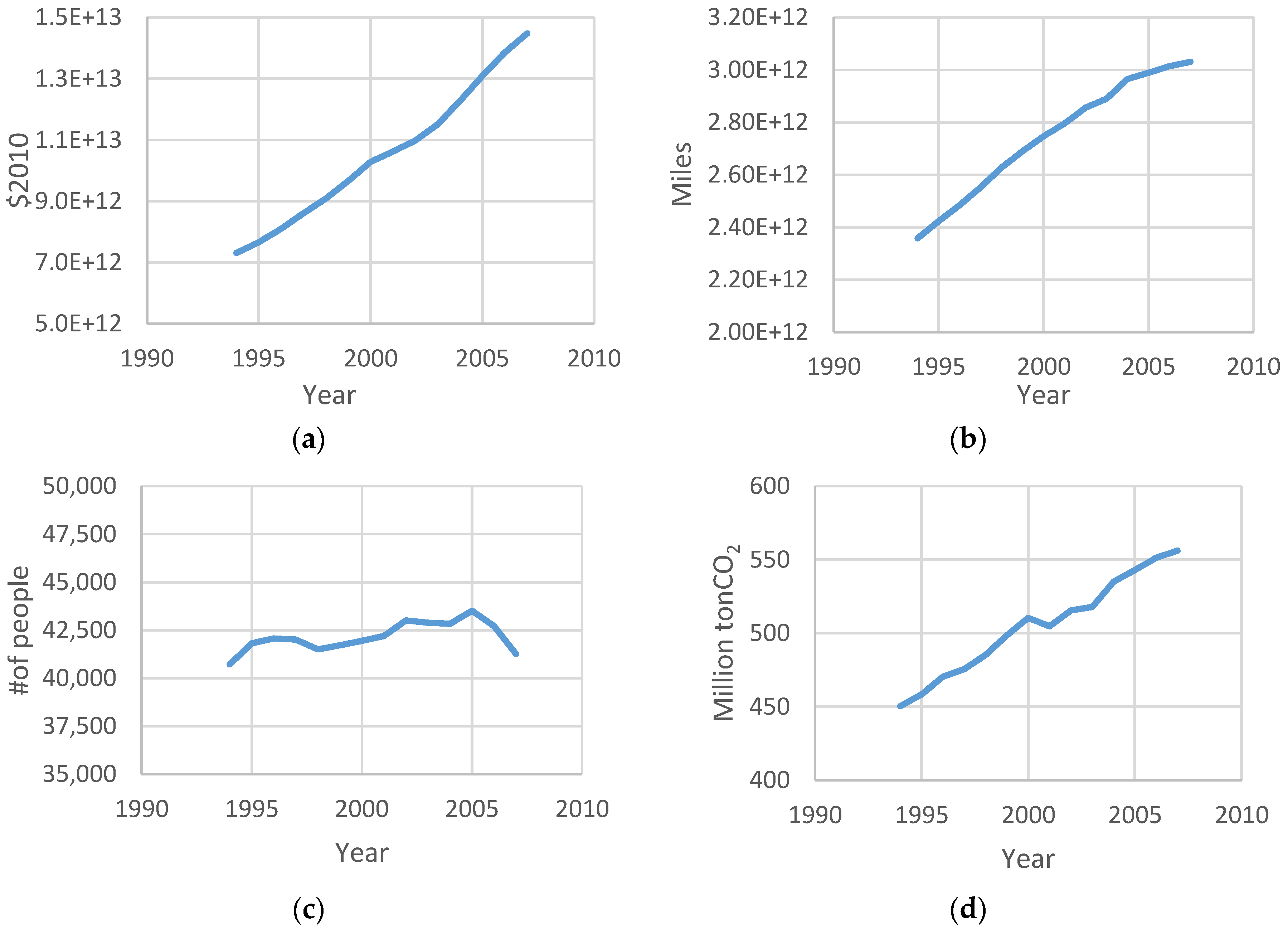
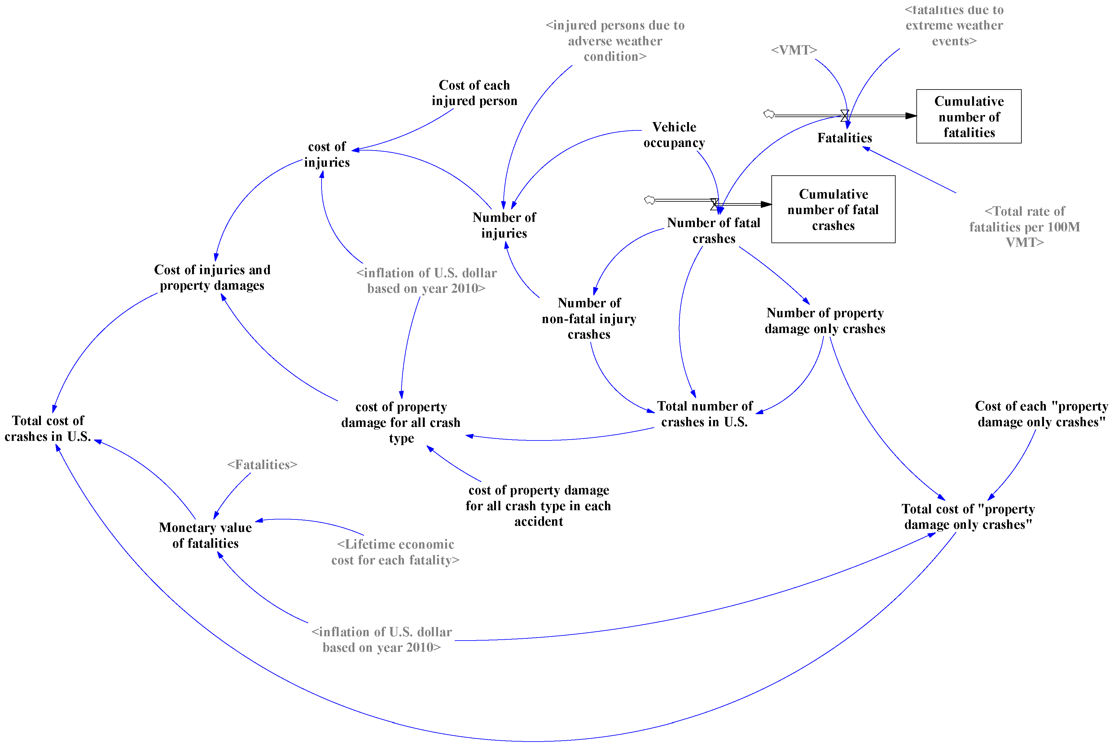
The economy is another important area to consider with respect to accidents and roadway safety in general. On the one hand, economic factors can have a positive impact on road safety, either through increases in highway system capacity that will thereby reduce roadway congestion, through improvements in vehicle safety or through various other road safety initiatives. On the other hand, however, road accidents and their associated injuries and fatalities can do significant damage to the economy. In 2010, there were almost 33,000 fatalities, 3.9 million injuries and damages to 24 million vehicles in the U.S. as a result of motor vehicle crashes [13], and according to the USDOT National Highway Traffic Safety Administration (NHTSA), the total economic cost of all of these negative impacts was estimated to be around $277 billion, or almost 1.9% of the total U.S gross domestic product (GDP); if quality of life valuations are added to this amount, the total cost increases to $871 billion. Climate change, extreme weather conditions and traffic congestion can also have a similarly tremendous effect on the economy, which (as shown in later sections) interacts directly and/or indirectly with other sectors.

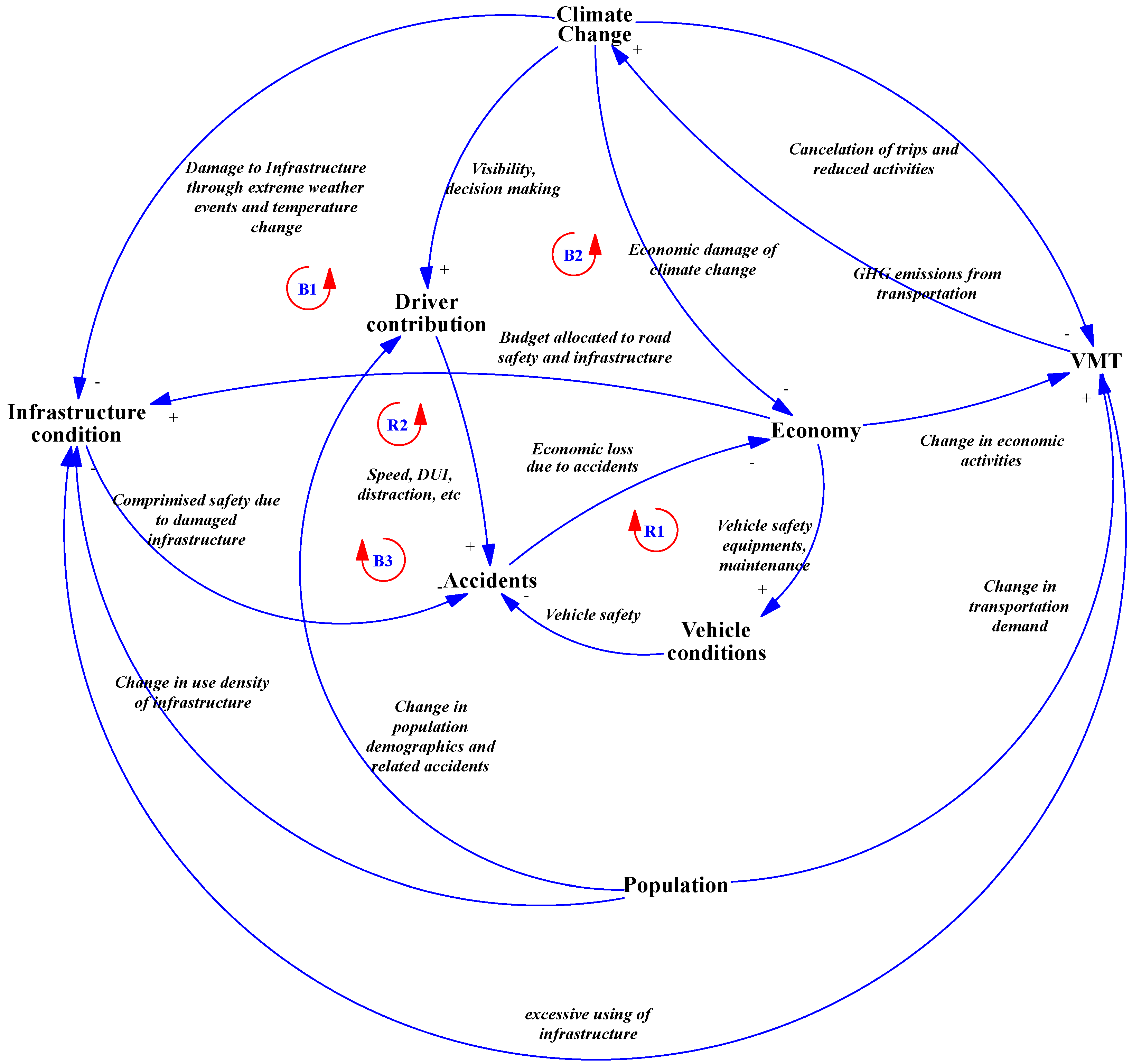
Effective management and proper policy making for complex systems requires a holistic understanding of the system as a whole, so that one can correctly interpret the interactions involved among different parameters in the system [14]. In order to achieve such an understanding and interpretation, it is necessary to integrate different branches of science to cover all or the most parameters in the system (or, at the very least, the most important thereof) in such a way that one can analyze each parameter individually and/or as part of the system given its interactions with other parameters. Integrated assessment modeling is a very useful tool for modeling complex systems, like those pertaining to environmental concerns, as well as related issues, such as climate change and predicting its associated future weather patterns, because such systems usually contain many subcomponents that each play their own major or minor roles within the system as a whole. Therefore, analyzing the actions and interactions among these components will be crucial to determining the behavior of the overall system, and this is also why analyzing such systems by focusing solely on single components is misleading and would result in wrong and/or incomplete solutions. The main focus of integrated assessment modeling is on analyzing the feedback processes through which the actions and interactions within the system take place [15]; integrated assessment modeling can integrate different branches of sciences for this purpose and can investigate the behavior of each component within the system, as well as each parameter’s individual behavior [16,17]. Finally, once a sufficiently accurate model has been developed with this methodology, the model is then used to inform policy making [15]. The most recently-developed integrated assessment modeling procedure is based on “system dynamics” modeling; the word “system” refers to the parameters interacting with each other and how these interactions will determine the behavior of the system, while the word “dynamics” refers to the time-dependency feature of the system [18], which will make time a particularly important parameter in the system dynamics (SD) modeling approach.

As mentioned earlier, one of the difficulties of investigating complex systems like road safety is that the interactions between different parameters playing any role within the system are very often neglected; this oversight becomes even more serious when the system and its parameters are dynamic in nature and when parameters are time dependent. Therefore, a comprehensive SD model to help policy makers find ways to reduce road fatalities and injuries should be capable of identifying all of the parameters related to road safety and should also take into account the relationships and interactions between all of these parameters. The SD modeling approach is evolving as an answer to these difficulties.

In the process of modeling any system, it is important to construct the model based on the behavior of the system in real-world situations and capture the interaction of the parameters affecting the system’s behavior in accordance with the real system. In previous studies, different sub-systems within the area of road safety were each investigated individually, regardless of their interactions with other parameters and sub-models. In contrast, this study aims to develop different sub-models to investigate each of these systems individually and/or in interaction with other systems. The ability of SD in moving beyond mere theory and entering into finding practical solutions and problem solving areas by considering the non-linear interaction of different sub-systems [19] and thereby proposing policies to improve the overall behavior of the system was the main motivation to tackle the issue of road safety by employing the SD modeling approach. In this regard, some basic understandings of the issue of road safety and roadway accidents may help in some level of judgment when applying qualitative assessments, but a comprehensive judgment of the whole system without going deeper into inner layers of road safety and investigating the way these layers interact with each other is difficult if not impossible.

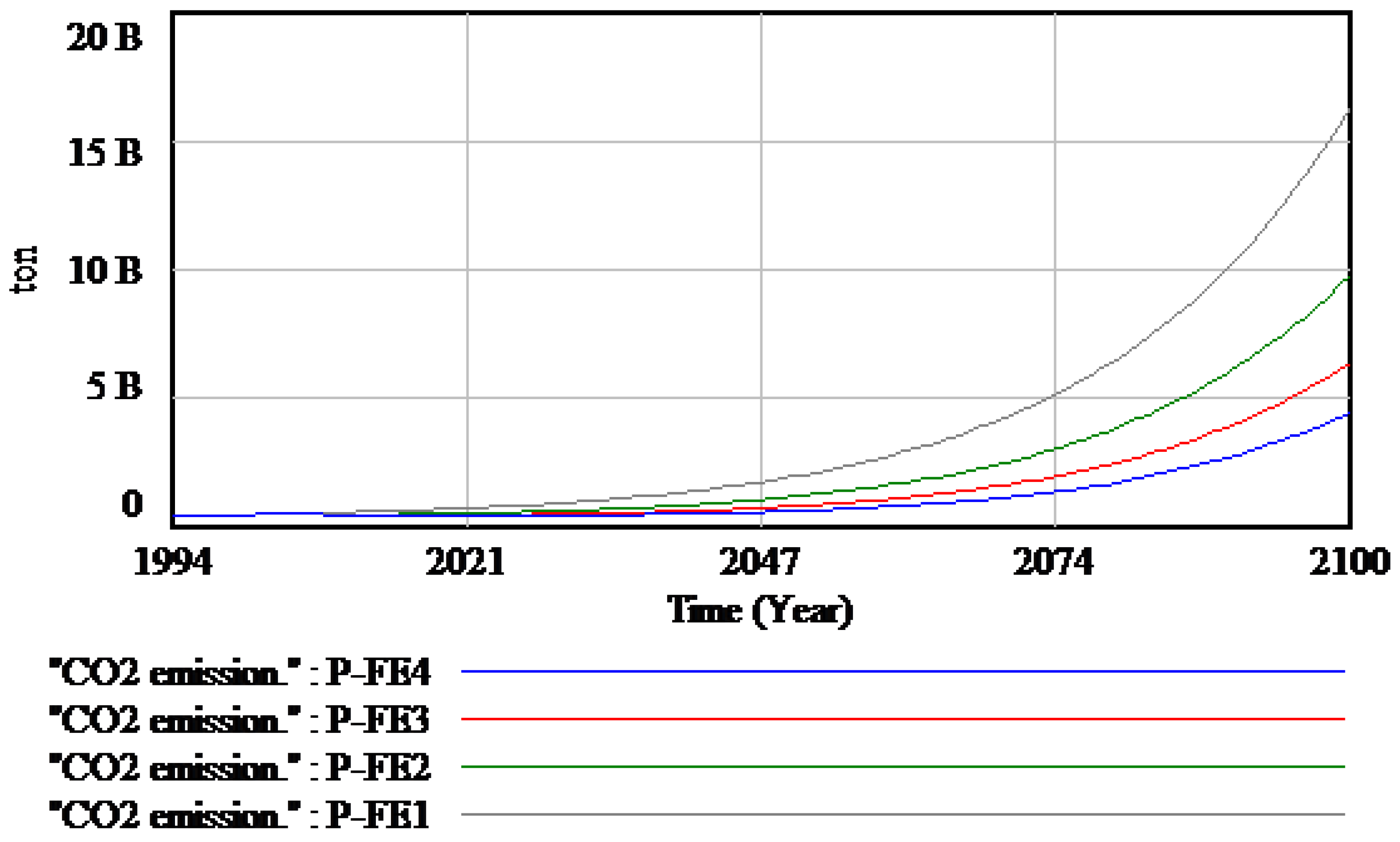
In order to reach the desired level of understanding of the behavior of the system, a throughout quantitative assessment is essential. Therefore, in this study, the main focus will be on developing models that can be used to quantitatively measure the impact of different applied scenarios on the overall outcome of the system. The results can then be used to predict the behavior of these different systems up to the year 2100, after which they will be used to test different scenarios to improve the behavior of the system and reduce the negative consequences of road accidents. The systems thinking approach adopted in this study can be used by researchers in other areas who are investigating complex systems with several dependent and independent sub-systems. As an example, when planning for smart cities, it is important to perform a detailed study on different components of the system, such as the smart economy, smart people, smart government, smart environment, etc. Each of these components of the smart city contains several other parameters within themselves that form the overall behavior of the system. In any of these sub-systems, not only the behavior of the sub-system itself should be investigated, but the overall behavior of the system, which is a resultant interaction of different parameters within the system, should be taken into account. In order to that, a systems thinking approach is an essential step in investigating the final outcome of the modeling process.

2. Model Development

2.1. Problem Identification

As stated in the Introduction (Section 1), the main purpose of this study is to provide a platform from which different scenarios can be tested to find the most efficient way(s) to increase road safety and to reduce the negative consequences of traffic accidents. For this purpose, a causal loop diagram is developed and presented in this section in order to identify the parameters of different sub-models, after which a stock and flow diagram will be constructed for each sub-model for quantification. In order to validate the constructed model, the reference modes used for vehicle miles traveled (VMT), number of crash fatalities, CO₂ emission and U.S. GDP are use and presented in Figure 1; these parameters are chosen because they play key roles in determining the other parameters.

2.2. Identification of Parameters

In order to create a causal loop diagram, the different parameters typically involved in road safety and transportation must be identified, and it must also be determined which parameters may or may not be directly connected, while indirect connections are typically revealed as separate series of one or more direct connections. For this purpose, the different parameters to be included in this causal loop diagram are introduced, organized by type (exogenous/“independent” versus endogenous/“dependent”) and briefly described in

Table 1. Key model parameters.

Parameter	Description	Type	Units
Vehicle condition	Vehicle safety-related factors (ANCAP rating)	Endogenous	-
Climate change	Extreme weather conditions (rain, hurricane, snow, extreme heat/cold, etc.)	Endogenous	-
Infrastructure condition	Road safety level and infrastructure equipment	Endogenous	-
Economy	Wealth and resources of a country or region	Endogenous	-
Population	The total number of people	Endogenous	-
Driver contribution	The accidents in which the driver’s fault will be the primary factor	Endogenous	-
VMT	Vehicle miles traveled	Endogenous	Miles
Accident	The total number of accidents happen in a certain period of time	Endogenous	-
Percentage of people saved by seat belt	Percentage of the passengers who saved their lives by fastening the seatbelt	Exogenous	-
Average added cost by FMVSS per vehicle	Average cost added to the cost of vehicle as a result of adding Federal Motor Vehicle Safety Standards	Exogenous	U.S. Dollars
Average travel mile	Average travelled distance per vehicle	Exogenous	Mile

. The validation of the inclusion of these parameters is performed in the next section.

2.3. System Conceptualization

In this part, a causal loop diagram is developed based on the parameters defined in Table 1. As discussed previously, one of the main advantages of the SD modeling approach compared to other modeling procedures is that it allows for a more in-depth investigation of the relationships and interactions between different parameters within the system through their associated feedback loops, which will be used to develop a causal loop diagram. Feedback loops are the most important characteristic of any system dynamic model, as these connectors will in fact determine how the results or outputs of a sector within the system should be used as an input for another sector in the system. These feedback loops can come with a positive or negative sign, depending on their overall effect after one full rotation within the loop. A positive (“reinforcing”) loop means the related parameters or sectors have the same overall increasing or decreasing trend, such that increasing or decreasing one parameter will result in a corresponding increase or decrease in the same parameter after a full rotation within the loop. Conversely, a negative (“balancing”) loop means that an increase or decrease in any parameter will have a decreasing or increasing effect, respectively, on the same parameter after a full rotation. A causal loop diagram (Figure 2) is constructed based on the parameters within the scope of this study, and a brief explanation on how these parameters affect each other is provided in Section 2.4.

2.4. Causal Loop Diagram Explanation

As can be seen in Figure 2, the constructed causal loop diagram consists of several reinforcing and balancing loops. These loops are indicated in the figure. B denotes the balancing loops, and R denotes the reinforcing loops. It is noteworthy to mention that all of the relationships between different parameters in this study are based on previous studies and the available literature in this field. In these studies, the authors either have proven the relationship between specific parameters through mathematical formulations or logically discuss the existence of the available relation in their study. Moreover, while constructing the casual loop diagram, we tried to rely on available data and discussions released by government agencies and accredited organizations to establish a connection between different parameters within the system. In this regard, historical data have played a very important role in order to project the behavior of the used parameters over time.

B1: Climate change-infrastructure condition-accidents-economy-VMT-climate change:

Increasing the extreme weather events will cause infrastructure to deteriorate, and this deterioration will increase accident rates. The increased number of accidents and accident-related fatalities and injuries will have a negative impact on the economy and decrease the VMT, reducing GHG emissions and thereby leading to less atmospheric temperature change, contributing less to extreme weather events in the long run [13,20,21,22,23].

B2: Climate change-driver contribution-accident rate-economy-VMT-climate change:

Increasing frequency of extreme weather conditions (rainfall, fog, snow, etc.) will increase the driver’s contribution to traffic accidents due to negative impacts on factors like visibility and decision making. This will increase the accident rate, which will have a negative impact on the economy and lower the VMT, as discussed earlier. Decreasing VMT rates will reduce GHG emissions and, consequently, less atmospheric temperature change and a reduced likelihood of extreme weather conditions in the future [13,20,24,25].

B3: Infrastructure condition-accident rate-economy-VMT-infrastructure condition:

Improving the condition of available infrastructure will result in fewer accidents and will thereby decrease the total economic burden of accidents. This increase in economic prosperity will result in an increase in travel demand and vehicle manufacturing, which will lead to an increase in VMT. However, the excessive use of infrastructure from this increased VMT will lead to greater infrastructure deterioration [13,20,26,27].

R1: Accident rate-economy-vehicle safety-accident rate:

Increasing the accident rate and/or the number of fatalities and injuries will have a negative impact on the economy, which, according to a report by the NHTSA, sometimes reaches up to 2% of the gross domestic product, which is a considerable amount. This reduction in economic prosperity will leave less money available for vehicle safety improvements; according to the NHTSA’s evaluation of the cost of the Federal Motor Vehicle Safety Standard (FMVSS) since 1975, by increasing the GDP (i.e., when the economy grows stronger), the vehicular safety index increases at the same time. Conversely, the resulting reductions in vehicle safety will increase the number and/or severity of future accidents, especially the latter [13,20,28].

R2: Economy-infrastructure condition-accident rate-economy:

A better economic situation will allow for better infrastructure conditioning due to the increased transportation sector share from the GDP. This can also help to increase highway mileage and capacity, reducing traffic congestion while also increasing infrastructure quality. These improvements in infrastructure will also reduce accident rates, making the economy less likely to suffer from the typical economic consequences associated with traffic accidents [13,20,27].

2.5. Model Formulation

The developed causal loop diagram will help to construct a stock and flow diagram for different systems in the next step of the SD modeling process. The following sub-models each contain the mathematical formulations of the relationships between different parameters, and each sub-model focuses on a specific area related to road safety, including sub-models to represent motor vehicle safety, highway systems and the environment, as well as two sub-models that mainly focus on economic losses due to transportation-related issues (Figure S1, shows how different sub-models are connected to each other and Figures S8, S9, S10, S11 and S15 show the number of fatalities due to distraction, DUI, extreme weather condition, driving below or above speed limit and aggressive driving respectively and Figure S17 shows the total rate of fatalities per 100 M VMT).

2.5.1. Economic Losses Sub-Model for Crashes with Respect to Fatalities, Injuries and Property Damage Only

This sub-model will use the output of another model that has already been submitted as a separate study. The total rate of fatalities per 100 M of VMT and the number of crashes with injury and property damage only are used to estimate the total economic cost of all types of crashes (Figure S7 shows the total number of road accident fatalities). This model can be seen in Figure 3 below. In this model, the number of crashes with fatalities, injuries and property damage only is obtained, and their economic losses are then calculated based on the information provided by the NHTSA as can be seen in

Table 2. Values of other parameters (source: NHTSA 2014).

Parameter	Value
Cost of each injured person	$37,524
Cost of property damage for all crash types in each accident	$13,836
Cost of each “property damage-only crashes”	$17,875
Lifetime economic cost for each fatality	$1,400,000
Average added cost by FMVSS per vehicle	$940
Vehicle occupancy	1.63

(Monetary value of roadway accident fatalities can be seen in Figure S14).

Different costs related to different crash types are obtained from NHTSA reports. In order to have more accurate values, the value of the U.S. dollar for different years has been calculated and multiplied by different costs, so that all costs are presented in 2010 U.S. dollars, as shown in Figure 4.

2.5.2. Motor Vehicle Safety Standards Sub-Model

This sub-model is used to model the role of vehicle safety standards in preventing roadway fatalities. The NHTSA has started to force the manufacturers of motor vehicles and equipment to apply certain safety standards rules in their products, which are accounted for in this model.

The Federal Motor Vehicle Safety Standards (FMVSS) aims to provide minimum safety performance requirements for motor vehicles and/or motor vehicle equipment. According to the NHTSA, these requirements are specified such “that the public is protected against unreasonable risk of crashes occurring as a result of the design, construction, or performance of motor vehicles and is also protected against unreasonable risk of death or injury in the event crashes do occur” [29].

As can be seen in Figure 5, this model seeks to estimate the number of lives saved through the implementation of the FMVSS based on the information provided in a report published by the NHTSA [30]. Based on this information, more than 328,000 lives have been saved between 1960 and 2002 by applying the FMVSS. With this in mind, a statistical model is used to estimate the number of lives saved by the implementation of the FMVSS based on the vehicular safety index; based on the model developed by the NHTSA, one can understand how many people would have died if the vehicles had not been equipped with these safety technologies. The number of lives saved by vehicle safety technologies can be obtained by a polynomial regression analysis based on the data provided by NHTSA, using the equation provided below:

Number of lives saved by vehicle safety technologies = −0.18786 × (vehicular safety index)² + 708.375 × (vehicular safety index) − 1240.

2.5.3. Highway System Capacity Sub-Model

This sub-model as can be seen in Figure 6 presents a more holistic view of the problem by concentrating on parameters like population (parameters “U.S. population and number of licensed driver” can be seen in Figures S16 and S13 respectively), VMT, vehicle fuel usage, traffic congestion, and so on (Detailed behavior of some of the involved parameters in this sub-model can be seen in Figures S2, S6 and S12. Also for the parameter “total cost added by FMVSS” see Figure S4).

In this model, the total number of vehicles is a function of the U.S. population and GDP and can be obtained using the formula below:

Total number of vehicles = (1.79197 × 10⁷) + 0.449554 × population + U.S. GDP × (6.52 × 10⁻⁶)

Congestion index = −2.25 + (2.69 × 10 ⁻⁶) × highway system capacity − (1.64 × 10⁻¹²) × VMT

(4.55 × 10⁻¹³) × (highway system capacity)² + (3.94 × 10⁻¹⁹) × highway system capacity × VMT

Annual wasted fuel due to congestion = (1.93025 × 10⁸) x (congestion index)² − (3.20771 × 10⁸) × (congestion index) + (1.4234 × 10⁸)

$$\mathrm{Fuel}\mathrm{use}=1.39311\times (\frac{\mathrm{VMT}}{\mathrm{Fuel}\mathrm{economy}\mathrm{policy}})+(3.71441\times {10}^9)$$

The fuel economy and average travel miles per vehicle are each entered as exogenous variables defined in the software VENSIM as a lookup table for different years. Furthermore, the total rate of fatalities per 100 M of VMT has already been calculated for different years; in this model, these fatality rates are simply multiplied by the VMT to obtain the total number of fatalities.

2.5.4. Environmental Impact Model

This model tracks the environmental impacts of the transportation sector. According to this model, the amount of CO₂ emitted from the transportation sector will be calculated for different years, after which the atmospheric temperature changes from the calculated CO₂ emissions will be obtained accordingly. Next, based on these atmospheric temperature changes, the changes in the applicable precipitation models will be investigated, specifically to see how increasing the atmospheric temperature will change the precipitation models based on the average precipitation patterns over the last 30 years. The data from the U.S. Department of Transportation Federal Highway Administration (FHWA) in the road weather management program will be used to construct this model.

As can be seen in Figure 7, this model will simulate the atmospheric temperature change over time and is also capable of calculating the economic loss due to climate changes by using the DICE (Dynamic Integrated Climate-Economy) model, as well as the economic damage function that was already calculated by [31]. This parameter will also be used later in the second economic sub-model (Figure 8) to calculate the economic damages to the GDP from atmospheric temperature change. Economic losses due to climate change are represented as damages to the GDP, which are usually related to damages associated with agricultural productivity, dislocations resulting from higher sea levels and dollar-equivalent costs, such as increases in mortality, morbidity and social disruption [32].

The next step is to see the consequences of this temperature change and its effect on road safety. For this purpose, another model is developed and presented in Figure 8 (The behavior of parameters “atmospheric temperature change” and “CO₂ in atmosphere” can be seen in Figures S3 and S5 respectively). In this sub-model, we tried to develop a model that is capable of estimating the number of days with extreme weather events up to the year 2100, based on the climate change models of the past 30 years. In terms of the effects of weather conditions on road safety, several variables seem to be more important than the others. For instance, although there have been several studies in this area to investigate the effects of weather conditions on road safety, it has been proven by this and other such methods that precipitation is the most important variable in this regard, while empirical data show that rain and snow can affect the frequency and severity of road accidents [33]. Therefore, in terms of extreme weather events, this model focuses primarily on precipitation model changes, such that the average increases in precipitation over time can be predicted based on estimations of the number of road accidents.

2.5.5. Economic Impact Sub-Model

Out of the different sub-models developed so far, one of the most important parameters considered in all four of the above-mentioned sub-models was the economy. Each of the economic parameters discussed in the previous sub-models will have an increasing or decreasing effect on the GDP, and these effects will all be combined in the final sub-model (Figure 9) to obtain the overall impact on the GDP.

As can be seen in the above figure, four parameters from the previous models determine the overall negative impacts of road transportation on U.S. GDP:

• The cost of crashes in U.S. includes the cost of crashes with fatality, injury and/or property damages only,
• The cost-benefit analysis of increasing the safety performance of motor vehicles by implementing the FMVSS,
• The economic benefits of decreasing the frequency and severity of road accidents due to increasing the safety level of motor vehicles,
• The economic benefits of decreasing the frequency and severity of road accidents due to increasing the safety level of motor vehicles and
• The annual highway congestion cost as a result of increasing the roadway congestion index.

3. Model Validation

Model validation is a very important part of the SD modeling process, as it uses a series of tests to guarantee the structural and behavioral accuracy of the developed model. Because the purpose of a system dynamic model is to reflect the real-world behavior of the modeled system, six key aspects of the model as a whole are tested to see if the model’s structure and behavior reflect the corresponding structure and behavior of the actual system. For this purpose, the results of the model will be compared with historical data (the reference modes from Figure 1). Without performing these validation tests, one cannot guarantee if the SD model represents the modeled system in reality, meaning that the model’s predictions and the proposed policies based on these predictions cannot be fully trusted to be reliable.

3.1. Model Structure Validity

In order to ensure that the structure of the developed SD model is adequate, five different types of tests are performed: structure verification test, parameter verification test, extreme condition test, boundary adequacy test and dimensional consistency test.

3.1.1. Structure Verification Test

The first test ensures that the parameters in the model and the simulated relationships between them do not contradict any currently-available knowledge of the system. For this purpose, this study used other published studies as references to model all of the parameters in the SD model, as well as their simulated relationships. These references have already been discussed in Section 2.4.

3.1.2. Parameter Verification Test

The second test is similar to the first test in that they are both qualitative rather than quantitative, and in that, they both have the same ultimate goal. However, this test more specifically seeks to determine whether or not the developed SD model is an adequate representation of the real system. For this purpose, all of the parameters mentioned in the explanation of the causal loop diagram and stock and flow diagrams (Section 2.4 and Section 2.5) have been checked to ensure that the modeled system does not in any way contradict currently-available knowledge of the real-world system.

3.1.3. Extreme Condition Test

The third test investigates the accuracy of the system’s structure by assigning extreme values to different parameters to see if the model demonstrates logically valid behavior based on the assigned extreme values. It is qualitatively observed that the model passed the extreme condition test by showing logical behavior.

3.1.4. Boundary Adequacy Test

The fourth test ensures that the boundaries of the developed model are defined in such a way that the model is well suited for the purposes of the study. In this study, the purpose of the model is to investigate the different parameters that affect roadway safety (motor vehicle safety, climate change, congestion, etc.), and from the different sub-models (Section 2.5), it can be observed that the goal of the system has been achieved by taking into account all of the aforementioned parameters.

3.1.5. Dimension Consistency Test

The fifth test seeks to verify the consistency of the units of the parameters used in the stock and flow diagrams (Section 2.5). From the different stock and flow diagrams developed in this study and their relevant equations, it can be seen that the units of the parameters are all consistent with each other.

3.2. Model Behavior Verification

The final test compares the output/results of the developed system dynamic model to real-world historical data to ensure that the datasets match closely enough to conclude that the model’s behavior accurately represents the behavior of the system in reality. For this purpose, as stated earlier, the results of the system for four key parameters are compared with available historical data (Figure 10) obtained from different reports and studies published by government organizations.

In this study, two statistical tests are also performed to compare the actual data with the outputs of the system: the one-way ANOVA test and the normality test.

Before the one-way ANOVA test can be performed, the normality test should be performed for both the actual data and the model output [34]; if the results show that both datasets are normal, then the one-way ANOVA test can be performed, but if not, then another test must be performed instead. The normality test is performed using SPSS software, and the results are shown in

Table 3. Normality test results.

		Tests of Normality
		Kolmogorov–Smirnov a			Shapiro–Wilk
		Statistic	df	Sig.	Statistic	df	Sig.
VMT	Model	0.088	14	0.2 *	0.970	14	0.879
	Data	0.124	14	0.200 *	0.931	14	0.319
GDP	Model	0.091	14	0.2 *	0.963	14	0.777
	Data	0.093	14	0.200 *	0.96	14	0.730
Fatalities	Model	0.089	14	0.2 *	0.97	14	0.875
	Data	0.123	14	0.200 *	0.98	14	0.974
CO2 emission	Model	0.122	14	0.2 *	0.936	14	0.364
	Data	0.096	14	0.200 *	0.962	14	0.752

* This is a lower bound of the true significance. ^a Lilliefors significance correction.

. It is obvious from Table 3 that all four parameters have passed the normality test for both the reference mode data and the SD model, since the sigma value is greater than 0.05 for all four parameters.

Now that the datasets have all been confirmed to be normal, the next step is to use the one-way ANOVA test to investigate whether or not there is a significant statistical difference between the reference modes and the SD model outputs. The results of the one-way ANOVA test are shown in Figure 11 for four different parameters.

As can be seen in Figure 11, the p-values for all four parameters are all greater than the selected confidence (α) value of 0.05, meaning that there is no significant statistical difference between the mean values of the obtained results from the SD model and those of the actual historical data.

4. Policy Analysis

The three main policy areas investigated in this study are fuel efficiency improvements, travel demand reduction and vehicle safety improvements. Any change in one or more of these areas can potentially affect other parts of the system, as well, so the investigation into the proposed policies will consequently have many interdependencies involved; in other words, these policy areas will function as explained in the causal loop diagram (Figure 2) and will have different impacts as opposed to the results of traditional modeling approaches.

Table 4. CO₂ emission for different values of fuel efficiency.

Policy Name	F.E.	2020	2050	2100
P-FE1	1	2.1 × 1011	3.35 × 1011	8.21 × 1011
P-FE2	1.25	1.69 × 1011	2.69 × 1011	6.57 × 1011
P-FE3	1.5	1.41 × 1011	2.24 × 1011	5.48 × 1011
P-FE4	1.75	1.22 × 1011	1.93 × 1011	4.7 × 1011

,

Table 5. Atmospheric temperature changes for different CO₂ emission reductions.

Policy Name	Reduction %	2020	2050	2100
P-WR1	0	1.78	1.46	1.11
P-WR2	25	1.08	0.89	0.69
P-WR3	50	0.58	0.55	0.51

,

Table 6. Vehicle miles travelled changes for different policies.

Policy Name	Reduction %	2020	2050	2100
P-ATM1	0	3.71 × 1012	5.94 × 1012	1.43 × 1013
P-ATM2	25	2.78 × 1012	4.45 × 1012	1.07 × 1013
P-ATM3	40	2.22 × 1012	3.56 × 1012	8.61 × 1012

and

Table 7. Vehicular safety index changes for different policies.

Policy Name	Increase %	2020	2030
P-ATM1	0	70.75	90.32
P-ATM2	10	77.83	99.35
P-ATM3	15	81.37	103.87

provide more specific details of the proposed policy options. The climate change-road safety-economy nexus is investigated by conducting the following policy tests:

• Increasing the vehicle fleet’s overall fuel efficiency by 25%, 50% and 75%,
• Reducing travel demand by 25% and 40% and
• Improving the vehicle safety index by 10% and 15%.

More detailed explanations of these policies are presented in the following sections along with their respective results.

5. Discussion and Results

In this section of the study, we tried to use the results of the analysis to investigate the effect of different policies on reducing the number of roadway accident and its consequences. These policies investigate the effect of certain parameters, such as fuel efficiency, extreme weather condition, travel demand and vehicular safety index, on the CO₂ emission rate, number of roadway accident’s fatalities, number of roadway accidents and number of lives saved, respectively.

5.1. Reducing CO₂ Emissions by Increasing Fuel Efficiency

After releasing the climate action plan, the government committed to a partnership with industries and stakeholders to develop new standards for increasing vehicle fuel efficiencies in order to reduce the negative consequences (health issues, climate change, etc.) of excessive fuel consumption in the U.S.

Based on this plan, the average fuel economy levels of new cars and light trucks should be doubled and increased up to 54.5 miles per gallon by 2025, which means a 100% increase in fuel efficiency compared to the present-day fuel economy. From the environmental and economic perspectives, this major increase in fuel efficiency will save $1.7 trillion at the pump and slash GHG emissions by as much as six billion metric tons over the respective lifetimes of the vehicles sold in almost 10 years [35]. For the purposes of this study, however, this model will be used to test relatively smaller fuel efficiency increases of 25%, 50% and 75%, to show how even small changes in fuel efficiency can compare to what was already planned for reducing fuel usage and GHG emissions. It is also possible to perform the policy analysis for smaller intervals of fuel efficiency increase of 1% instead of 25%, but what has been seen in the results is the same decreasing trend. Therefore, instead of showing the whole analysis for every 1% for fuel efficiency increase, the initial, final and two median values (0%, 25%, 50% and 75%) were assigned to the fuel efficiency increase.

As can be seen in Table 4, continuing the current situation will cause the CO₂ emitted from the transportation sector to continuously increase until 2100, meaning that CO₂ emissions will increase to 8.21 × 10¹¹ in 2100 from 4.44 × 10⁸ in 2015. The first policy test is to investigate the effects of increasing fuel efficiency (F.E) by different values in order to reduce fuel usage and, by extension, reduce CO₂ emissions. For this purpose, four different values (Table 4) have been considered in order to test their effects on CO₂ emission.

In Figure 12, the effect of different fuel economies can be seen in CO₂ emissions.

After analyzing the model, the effects of vehicle fuel efficiency changes alone on atmospheric temperature change were found to be not as important as those other parameters. One reason for that is because the total “rate of CO₂ emissions from the rest of the world” has a much larger value compared to CO₂ emissions solely from the U.S. transportation sector, and so, the effect of changing CO₂ emissions in the U.S. cannot be clearly recognized in this case. The fact is that any improvement in fuel efficiency would make a minimal change on the total CO₂ emission stock due to two main reasons; first, because the U.S. is responsible for 16% of global CO₂ emission and the transportation sector emits 26% of the total CO₂ emitted to the atmosphere [36], which indicates that the total share of US transportation emissions in the world is about 4.4%. As can be seen, in the best case, improving fuel efficiency even by 50% in the U.S. can have a very negligible impact on the global CO₂ emission worldwide and consequently on global warming issue. Second, all of the above-mentioned numbers are rates rather than stock (total CO₂ emission to the atmosphere). This system works pretty much like a bathtub with inflow/faucet (annual emission rates) and outflow/drain (carbon sequestration). Therefore, as long as the inflow is greater than the outflow, global warming will continue its increasing trend. Moreover, reducing inflow will only make a difference as long as it became smaller than the outflow. What causes global warming is the atmospheric concentration (the stock), so even if all CO₂ emissions stop now, global warming will still continue until the CO₂ concentration lowers at some level through carbon sequestration, which also takes time (delays in this system).

In order to clarify this further in this study, another policy is tested based on worldwide CO₂ emission reductions, reducing the global CO₂ emission targets of 25% (WR1) and 50% (WR2) in order to see if such worldwide reduction goals have any significant effects on temperature change or on road safety. Again, in this scenario, a 0% reduction indicates what would happen if no action is taken to reduce GHG emissions. The results of this analysis can be seen in Table 5.

As a direct result of changes in the CO₂ emission rate and temperature, the number of roadway accidents and fatalities due to extreme weather conditions can change. This effect is obvious in Figure 13.

5.2. Travel Demand Reduction

There is a growing concern about the negative impacts of transportation systems and their respective side effects, including GHG emissions, traffic congestion, air pollution, and so on. The parameter vehicle miles traveled (VMT) is usually used in order to address these concerns. There have been several discussions about finding ways to reduce the VMT while still maintaining the economic growth and social activities at the same rate. This goal can be achieved by increasing the use of other types of transportation besides motorized passenger vehicles, including walking, cycling, using public transportation, etc. [37]. This has become a widely-discussed topic, especially knowing that the VMT and the GDP (as an economic indicator) are strongly coupled, so there should be an intermediate way in which the maximum effort is made to reduce the VMT without comprising economic growth.

Based on the above-listed background on attempts to reduce VMT, states and city areas are required to set target VMT reductions that they plan to achieve within a specified time limit. Based on a report published by the FHWA, different states have set different targets for VMT reduction; for example, Denver, the Sacramento area, the San Francisco Bay area and certain other areas have settled on target VMT reductions of 10% by 2035, while Seattle has set its target VMT reduction to 50% by 2050 [37]. It can therefore be concluded that the VMT reduction targets for different areas may vary based on their available infrastructures and accommodations. In this study, the target VMT reduction is set as the average target VMT reductions of different states.

The next scenario attempts to quantify the effects of travel demand reduction on VMT, as well as its effects on the number of fatalities and on other parameters involved in this system. For this purpose, two specific scenarios (Table 6) were simulated as a target travel demand reduction of 25% (ATM2) or 40% (ATM3). The first scenario (0% reduction) indicates the situation if the current increasing trend of VMT continues as is.

As can be seen in Table 6, the third scenario can reduce the VMT by almost six billion miles. This huge reduction in miles traveled will result in a reduction in the number of fatalities (as is shown in Figure 14) and injuries and will make the roads safer by reducing the congestion index.

5.3. Vehicular Safety Index Increase

There is a strong consensus that vehicle safety improvements are crucial to reducing the number of fatalities and injuries in road accidents. In different studies and reports published by government or international organizations, different technologies and tools were introduced that are still helpful in increasing the vehicle safety. For example, in a report published by the World Health Organization (WHO), one chapter encourages the harmonization of the relevant global standards to accelerate the uptake of new vehicle safety technologies [38].

Early vehicle safety efforts were focused on increasing the capability of vehicles to withstand a crash by improving the structural design, materials and safety systems of the vehicles in question [39]. This step starts by ensuring that every vehicle has certain basic safety performance measures, such as seatbelts and airbags, and continues to promote the more widespread use of crash avoidance technologies, such as electronic stability controls and anti-lock braking systems [38]. These technologies aim to prevent crashes from occurring in the first place and can in fact make vehicles more intelligent as they become more able to sense and communicate with other vehicles and with roadside infrastructure [39]. In order to promote such systems, policy makers are considering offering incentives for manufacturers to employ these technologies; for example, the USDOT recognizes the need to reward commercial motor carriers who deploy safety technologies in their fleet and even for considering investing in V2V (vehicle to vehicle) and V2I (vehicle to infrastructure) communication programs [39,40].

In this study, the increasing vehicle safety scenario is focused on decreasing the road accidents and the number of fatalities and injuries through increasing the safety index of the vehicles. For this purpose, three different scenarios have been tested to see their effect on increasing the safety of the passengers. The results can be seen in Table 7 and Figure 15 below.

6. Conclusions

In this study, the climate change-road safety-economy nexus is investigated, and several related policies are analyzed to explore ways to reduce the accident rate in the U.S. The policies aiming to increase fuel efficiency reduce the transportation-related emissions. However, reducing transportation-related emissions has negligible impact on slowing down the atmospheric temperature rise, which cannot eliminate or reduce the negative effects of climate change on road safety. Hence, as a second policy area, extreme world-wide emission reduction policies are explored to show how climate change affects the road safety. According to this extreme policy area, reducing GHG emissions worldwide can significantly reduce the fatalities resulting from road accidents thanks to fewer extreme weather events, infrastructure damage and the distraction of drivers. As a second policy area, reducing the travel demand was investigated, which results in a significant decrease in the rate of fatalities. This policy area is found to be a more effective way of reducing accidents compared to the policies aiming to increase fuel efficiency. Lastly, the effects of improving the vehicle safety index on recuing fatalities are investigated. Improving the vehicle safety index can significantly reduce the number of fatalities and should be prioritized.

In the continuation of this study, we will try to put more emphasis on policy analysis by examining different parameters and assigning broader ranges of values to the parameters through performing multivariate analysis. As the system dynamic modeling approach is no longer limited to modeling uncomplicated straightforward phenomena, rather, it is capable of conducting models with uncertainty and deep complexity by combining multivariate analysis and the SD modeling approach and to investigate all plausible outcomes and policies in a given range of model parameters [17,41].

References

1. Hughes, B.P.; Newstead, S.; Anund, A.; Shu, C.C.; Falkmer, T. A review of models relevant to road safety. Accid. Anal. Prev. 2014, 1–21. [Google Scholar] [CrossRef] [PubMed]
2. Breen, A.; Seay, J. World Report on Road Traffic Injury Prevention; World Health Organization: Geneva, Switzerland, 2004. [Google Scholar]
3. Miang, Y.; Love, P.E.D. Methodological application of system dynamics for evaluating traffic safety policy. Saf. Sci. 2012, 50, 1594–1605. [Google Scholar]
4. Pisano, P.; Goodwin, L.; Stern, A. Surface Transportation Safety and Operations: The Impacts of Weather within the Context of Climate Change. In The Potential Impacts of Climate Change on Transportation; Transportation Research Board: Washington, DC, USA, 2001; pp. 1–22. [Google Scholar]
5. Yu, R.; Abdel-Aty, M. Analyzing crash injury severity for a mountainous freeway incorporating real-time traffic and weather data. Saf. Sci. 2014, 63, 50–56. [Google Scholar] [CrossRef]
6. Egilmez, G.; McAvoy, D. Benchmarking road safety of U.S. states: A DEA-based Malmquist productivity index approach. Accid. Anal. Prev. 2013, 53, 55–64. [Google Scholar] [CrossRef] [PubMed]
7. Das, A.; Abdel-Aty, M. A combined frequency–severity approach for the analysis of rear-end crashes on urban arterials. Saf. Sci. 2011, 49, 1156–1163. [Google Scholar] [CrossRef]
8. Champaneri, A.; Guarino, J. Factors Involved in Fatal Crashes. Available online: http://fleetresearch.com/2010_Factors_in_Fatal_Vehicle_Crashes.pdf (accessed on 16 January 2017).
9. Abdel-Aty, M.; Pande, A. Identifying crash propensity using specific traffic speed conditions. J. Saf. Res. 2005, 36, 97–108. [Google Scholar] [CrossRef] [PubMed]
10. Karl, T.R. Global Climate Change Impacts in the United States; Cambridge University Press: Cambridge, UK, 2009. [Google Scholar]
11. Transportation Research Board Special Report 290, Potential Impact of Climate Change on U.S Transportation. 2008. Available online: www.TRB.org (accessed on 14 January 2017).
12. TRB Transportation Research E-Circular E-C152. Adapting Transportation to the Impacts of Climate Change; Transportation Research Board: Washington, DC, USA, 2011. [Google Scholar]
13. Blincoe, A.B.L.; Zaloshnja, E.; Miller, T. The Economic and Societal Impact of Motor Vehicle Crashes; National Highway Traffic Safety Administration: Washington, DC, USA, 2010.
14. Kelly (Letcher), R.A.; Jakeman, A.J.; Barreteau, O.; Borsuk, M.E.; ElSawah, S.; Hamilton, S.H.; Henriksen, H.J.; Kuikka, S.; Maier, H.R.; Rizzoli, A.E.; et al. Selecting among five common modelling approaches for integrated environmental assessment and management. Environ. Model. Softw. 2013, 47, 159–181. [Google Scholar] [CrossRef]
15. Davies, E.G.R.; Simonovic, S.P. Global water resources modeling with an integrated model of the social–economic–environmental system. Adv. Water Resour. 2011, 34, 684–700. [Google Scholar] [CrossRef]
16. Ercan, T.; Onat, N.C.; Tatari, O. Investigating carbon footprint reduction potential of public transportation in United States: A system dynamics approach. J. Clean. Prod. 2016, 133, 1260–1276. [Google Scholar] [CrossRef]
17. Ercan, T.; Onat, N.C.; Tatari, O.; Mathias, J.-D. Public transportation adoption requires a paradigm shift in urban development structure. J. Clean. Prod. 2016, 142, 1789–1799. [Google Scholar] [CrossRef]
18. Akhtar, M.K. A System Dynamics based Integrated Assessment Modelling of Global-Regional Climate Change: A Model for Analyzing the Behaviour of the Social-Energy-Economy-Climate System; The University of Western Ontario: London, ON, Canada, 2011. [Google Scholar]
19. Kumar, S.N.; Umadevi, G. Application of System Dynamic Simulation Modeling in Road Safety. In Proceedings of the 3rd International Conference on Road Safety and Simulation, Indianapolis, IN, USA, 14–16 September 2011.
20. Blincoe, R.S.L.; Seay, A.; Zaloshnja, E.; Miller, T.; Romano, E.; Luchter, S. The Economic and Societal Impact Of Motor Vehicle Crashes; National Highway Traffic Safety Administration: Washington, DC, USA, 2000.
21. Koetse, P.R.J. The impact of climate change and weather on transport: An overview of empirical findings. Transp. Res. Part D 2009, 14, 205–221. [Google Scholar] [CrossRef]
22. Environmental Protection Agency. U.S transportation sector Greenhouse Gas Emission; Environmental Protection Agency: Washington, DC, USA, 2013.
23. Zimmerman, R. Global Climate Change and Transportation Infrastructure: Lessons from the New York Area; Transportation Research Board: Washington, DC, USA, 2003; pp. 1–11. [Google Scholar]
24. Mills, B.B.; Andrey, J. Climate Change and Transportation: Potential Interactions and Impacts; Transportation Research Board: Washington, DC, USA, 2003; pp. 1–12. [Google Scholar]
25. Kilpeläinen, M.; Summala, H. Effects of weather and weather forecasts on driver behaviour. Transp. Res. Part F Traffic Psychol. Behav. 2007, 10, 288–299. [Google Scholar] [CrossRef]
26. Flahaut, B. Impact of infrastructure and local environment on road unsafety. Accid. Anal. Prev. 2004, 36, 1055–1066. [Google Scholar] [CrossRef] [PubMed]
27. Noland, R.B. Traffic fatalities and injuries: The effect of changes in infrastructure and other trends. Accid. Anal. Prev. 2003, 35, 599–611. [Google Scholar] [CrossRef]
28. Tarbet, J. Cost and Weight Added by the Federal Motor Vehicle Safety Standards for Model Years 1968–2001 in Passenger Cars and Light Trucks. Available online: https://one.nhtsa.gov/cars/rules/regrev/evaluate/809834.html (accessed on 14 January 2017).
29. NHTSA. Federal Motor Vehicle Safety Standards and Regulations. U.S. Department of Transportation, 1999. Available online: http://www.nhtsa.gov/cars/rules/import/FMVSS (accessed on 14 January 2017). [Google Scholar]
30. Kahane, C.J. Lives Saved by the Federal Motor Vehicle Safety Standards and Other Vehicle Safety Technologies, 1960–2002 Passenger Cars and Light Trucks with a Review of 19 FMVSS and Their Effectiveness in Reducing Fatalities, Injuries and Crashes. Available online: https://one.nhtsa.gov/cars/rules/regrev/evaluate/809833.html (accessed on 14 January 2017).
31. Pindyck, R.S. Modeling the Impact of Warming in Climate Change Economics. Natl. Bur. Econ. Res. Steckel. 2010. [Google Scholar] [CrossRef]
32. Pindyck, R.S. Modeling the Impact of Warming in Climate Change Economics. In Economics of Climate Change: Adaptations Past Present, the National Bureau of Economics Research-Libecap and Steckel; University of Chicago Press: Chicago, IL, USA, 2011; p. 47. [Google Scholar]
33. Koetse, M.J.; Rietveld, P. The impact of climate change and weather on transport: An overview of empirical findings. Transp. Res. Part D 2009, 14, 205–221. [Google Scholar] [CrossRef]
34. Egilmez, G.; Tatari, O. A dynamic modeling approach to highway sustainability: Strategies to reduce overall impact. Transp. Res. Part A 2012, 46, 1086–1096. [Google Scholar] [CrossRef]
35. The White House. Improving the Fuel Efficiency of American Trucks; The White House: Washington, DC, USA, 2014.
36. US EPA. GHG Equivalencies Calculator—Calculations and References. United States Environmental Protection Agency, 2015. Available online: http://www.epa.gov/energy/ghg-equivalencies-calculator-calculations-and-references (accessed on 19 February 2016). [Google Scholar]
37. Ecola, L.; Wachs, M. Exploring the Relationship between Travel Demand and Economic Growth; Transportation Research Board: Washington, DC, USA, 2012. [Google Scholar]
38. World Health Organization. Decade of Action for Road Safety 2011–2010; World Health Organization: Geneva, Switzerland, 2011. [Google Scholar]
39. United States Department of Trasportation. Roadway Safety Plan; United States Department of Trasportation: Washington, DC, USA, 2010.
40. Alirezaei, M.; Noori, M.; Tatari, O. Getting to net zero energy building: Investigating the role of vehicle to home technology. Energy Build. 2016, 130, 465–476. [Google Scholar] [CrossRef]
41. Pruyt, E. Dealing with uncertainties? combining system dynamics with multiple criteria decision analysis or with exploratory modelling. In Proceedings of the the 25th International Conference of the System Dynamics Society, Boston, MA, USA, 29 July–2 August 2007.
Figure 1. Reference mode (source: National Highway Traffic Safety Administration (NHTSA) 2014) (a) U.S. GDP; (b) vehicle miles traveled (VMT); (c) number of fatalities; (d) CO2 emissions.
Systems 05 00006 g001
Figure 2. Causal loop diagram.
Systems 05 00006 g002
Figure 3. Economic losses’ sub-model.
Systems 05 00006 g003
Figure 4. U.S. dollar values in 2010 U.S. dollars.
Systems 05 00006 g004
Figure 5. Motor vehicle safety sub-model.
Systems 05 00006 g005
Figure 6. Transportation system sub-model.
Systems 05 00006 g006
Figure 7. Environmental impact sub-model (GHG emissions).
Systems 05 00006 g007
Figure 8. Environmental impact sub-model (precipitation and*-+ + weather).
Systems 05 00006 g008
Figure 9. Economic impact sub-model.
Systems 05 00006 g009
Figure 10. Behavioral validation results: (a) U.S GDP; (b) VMT; (c) Number of fatalities; (d) CO2 emissions.
Systems 05 00006 g010
Figure 11. Results of the one-way ANOVA test.
Systems 05 00006 g011
Figure 12. CO2 emissions rate for different fuel efficiency scenarios.
Systems 05 00006 g012
Figure 13. Fatalities due to extreme weather changes for different policies.
Systems 05 00006 g013
Figure 14. Number of road accident fatalities for different policies.
Systems 05 00006 g014
Figure 15. Number of lives saved by vehicle safety technologies for different policies.
Systems 05 00006 g015