Article

Utility Perception in System Dynamics Models †

1
New Mexico Water Resources Research Institute, New Mexico State University, Las Cruces, NM 88003, USA
2
Department of Mechanical Engineering, Worcester Polytechnic Institute, Worcester, MA 01609, USA
*
Author to whom correspondence should be addressed.
This paper is an extended version of our paper published in Langarudi, S.P.; Bar-On, I. Utility Perception in System Dynamics Models. In Proceedings of the 35th International Conference of the System Dynamics Society, Cambridge, MA, USA, 16–20 July 2017; p. 5.
Systems 2018, 6(4), 37; https://doi.org/10.3390/systems6040037
Submission received: 30 July 2018 / Revised: 13 September 2018 / Accepted: 26 September 2018 / Published: 28 September 2018
(This article belongs to the Special Issue Theory and Practice in System Dynamics Modelling)

Abstract

:
The utility perceived by individuals is believed to be different from the utility experienced by that individual. System dynamicists implicitly categorize this phenomenon as a form of bounded rationality, and traditionally employ an exponential smoothing function to capture it. We challenge this generalization by testing it against an alternative formulation of utility perception that is suggested by modern theories of behavioral sciences. In particular, the traditional smoothing formulation is compared with the peak–end rule in a simple theoretical model as well as in a medium-size model of electronic health records implementation. Experimentation with the models reveals that the way in which utility perception is formulated is important, and is likely to affect behavior and policy implications of system dynamics models.

1. Introduction

Decisions regarding preferences involve the utility derived from the preferred outcome. Utility in this context can be experienced utility, remembered (perceived) utility, or decision utility, and there can be notable differences between them [1,2,3]. Experienced utility is the pleasure (or its opposite) that we gain from an action at any moment. Remembered utility is the utility an individual perceives through mental filters. Decision utility is manifested by revealed preferences or the choices the individual makes [4]. For remembered utility and thus decision utility, it has been shown that it is frequently disproportionally affected by the peak and end values of an experience, while duration of experience seems to be less significant—a behavior that is labeled by Fredrickson and Kahneman [5] as “duration neglect” or peak–end rule [6,7].
System dynamics (SD) models represent utility-based decisions using the construct of perceived information. In SD, utility-based decisions use information as one of the inputs. It is recognized that this is not instantaneous information, but rather information that is modified over time, leading to the concept of perceived information. Perceived information is modeled as a smoothing process, as will be described further in the market growth model example later. The utility perception concept is implicit and perhaps too abstract in the SD representation. This representation has two potential issues. First, it merges the process of utility perception with the outcomes of the perception, that is, decision utility (compare the highlighted boxes in Figure 1). That is, system dynamics models focus merely on the perception process and ignore the formation of decision utility. However, remembered (perceived) utility can be different from decision utility, although the latter is usually a direct consequence of the former (perhaps with a delay involved), ceteris paribus.
Second, the representation does not distinguish between “utility perception” and managerial “information perception”. Managerial information is usually perceived through formal means, such as data records and analysis. It is reasonable to assume that an exponential averaging mechanism captures the information perception with adequate accuracy, because in such a setting, the agents can review the historical information and correct their decisions if necessary. In contrast, experienced and perceived utility include components such as joy, pain, anger, sadness, etc., which are not necessarily based solely on formal means. Traditionally, in system dynamics, perceived utility (or perceived preference) is formulated as a first-order smooth, in the same fashion as the perceived information is formulated. One classic example is the reaction of customers to long delivery delays, as appeared in the market growth model [8]. In this model, both managers and customers perceive the delivery delay through a first-order smooth, while the only distinction between the two is that the customer information perception takes more time. The process of utility perception by customers from delivery time is assumed to be implicit in the information perception, as if customers, like managers, receive spreadsheet reports at regular intervals telling them how they feel about the delivery time. Mathematically, customer satisfaction from delivery time (x) is perceived ( x ¯ ) with a delay (T) 1.
x ¯ t + d t = x ¯ t + x t x ¯ t T · d t
This perception of utility, as formulated in traditional SD models, is usually symmetrical and uniformly smoothed over a particular time period. As such, it is akin to the sum of experienced utilities. The representation of utilities used in system dynamics models (shown in Equation (1)) is developed from the use of smooths in the formulation of perceived information. Perceived information includes an information delay (smooth) of the actual information to represent the discrepancy between actual information and what we represent as the information perceived by an agent at the moment of information reception. This formulation implies that the duration of experience plays a key role in the formation of perception. We can rewrite Equation (1) as follows:
x ¯ t + d t = ( 1 α ) x ¯ t + α x t ,
α = d t T < 0.25 .
Equation (2) indicates that perceived utility (information) is a weighted average of two arguments. The first argument is the average perceived utility in the past—thus taking duration of the experience into account. The second argument is the utility perceived from the last moment of the experience—which is called “end value”, as we will see later. The weight of the arguments depends on our selection of averaging time (T). However, α can never be greater than 25%2. This means that the smoothing formulation always gives at least 75% (i.e., 1 α ) of the weight to the average perceived utility in the past which represents duration of the experience.
An alternative mechanism for decision utility formation may lead to a disregard of time duration and emphasis on extreme values and more recent experiences as formulated in the peak–end rule3. The peak–end rule was originally documented for pain experienced during medical procedures [7], where patients were asked during the procedure to rate the pain that they experienced during the procedure in fixed intervals. After the procedure, the patients were asked to rate the total amount of pain that they had experienced during the procedure. The results indicated that this later measure was not reflective of the sum of the values during the procedure, but was better represented by the average of the peak and last values—thus, the term “peak–end value”. This peak–end rule has since been documented for a range of situations [11,12,13]. Implementation of a peak–end formulation for preferences gives the following expression:
U = P + E 2 ,
where U is perceived (remembered) utility, P is utility from the most intense experience (PEAK), and E is utility from the most recent experience (END).
This formulation is substantially different from that of an averaged expression of utility (represented by Equation (2)). Although both of these equations are weighted averages of two arguments (one of which is “end value”), they differ in the second argument. For the smoothing formulation, the second argument is an average of past utilities, while for the peak–end formulation, it is the most extreme (peak) utility that is experienced in the past. Furthermore, the weight of the arguments in the peak–end formulation (corresponding to α in Equation (2)) is always constant and equal to 50%. Thus, the peak–end formulation gives greater weight to the end value than does the smoothing formulation in the averaging function. It also ignores duration of the experience and gives the remainder of the weight to only one instant of history, which is when the peak utility happens.
In this paper, we pose the question of whether or not alternative formulations of utility perception for preference decisions will substantially alter the results of the modeling exercise, and thus of the corresponding policy recommendations. We start with a simple theoretical model that focuses on a comparison between the traditional perceived information (smooth) and the peak–end rule formulation. This is presented in the following section. Next, the rule is applied to a medium-size system dynamics model that has been already developed for addressing technological changes in healthcare settings [14]. The last two sections discuss the implications and conclude the paper.

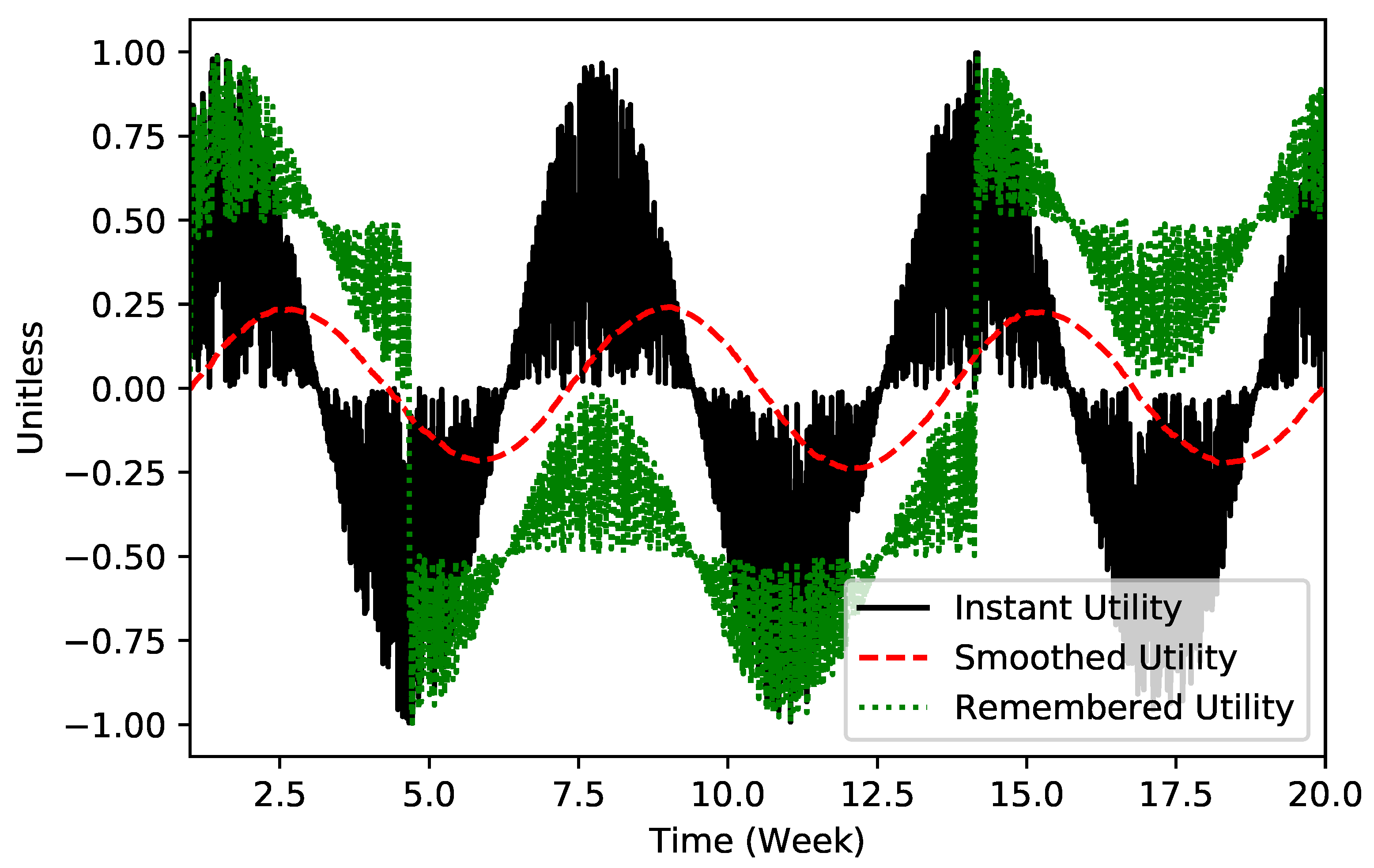
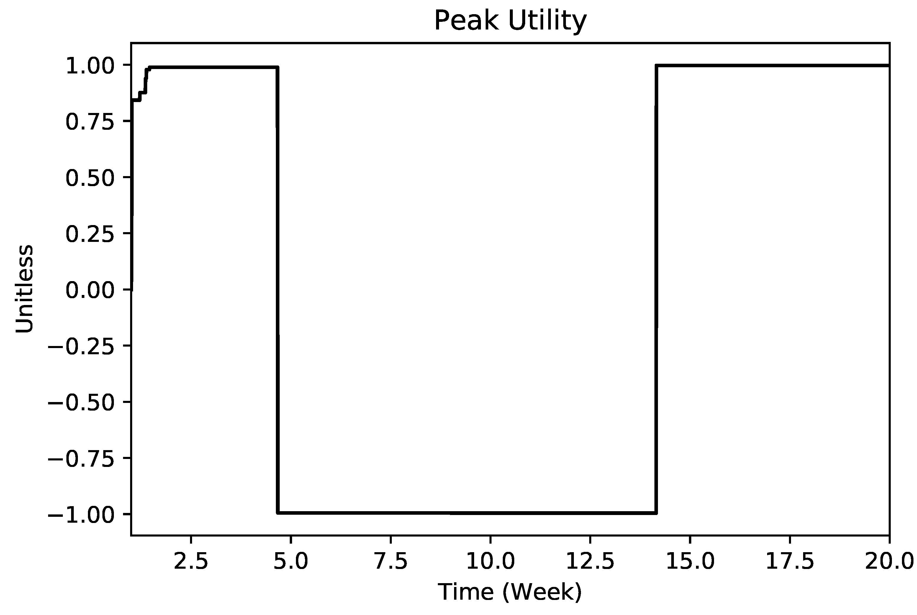
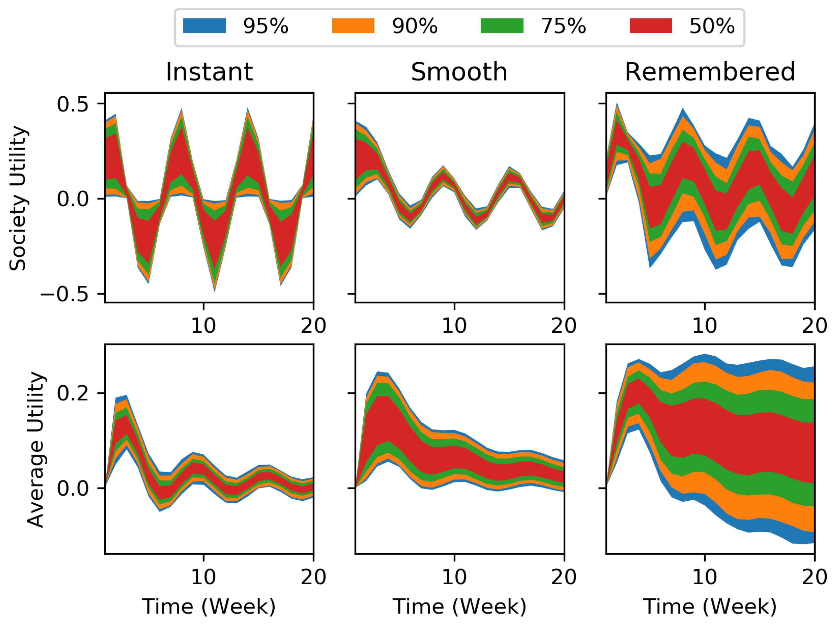
2. Peak–End Rule in a Theoretical Setting

In this section, we examine the peak–end value formulation for a very simple example model and compare the results with those of the smoothing formulation. The model diagram is shown in Figure 2. Equations of the model can be found in Appendix A. The model starts with an assumed “instant utility” that can be exposed to a test input. This is the exact utility individuals experience from an event, so it is an equivalent of “experienced utility”. But what is perceived by them as “perceived utility” (or “remembered utility”) might be different. As mentioned in Section 1, system dynamics models calculate this discrepancy between actual and perceived utility using simple smoothing. This is shown by “smoothed utility” in Figure 2. As mentioned above, utility perception might be processed differently. According to the peak–end rule, utility that individuals perceive (“remembered utility”) is an arithmetic average of “peak utility” and “end utility”. Peak utility is the utility individuals gain from their most intense experience of an event. End utility, on the other hand, is the utility that individuals gain from their most recent experience of that particular event. In the model, we also calculate the average of each utility perception (“average smoothed utility” and “average remembered utility”) to better evaluate the effect of each on the overall state of the system.
To test the behavior of the modeled system, a sine function together with a uniform random function was used. As presented by Equation (5), this function creates an oscillatory behavior with random irregularity for the input (“instant utility”):
u t = p t sin ( t ) .
Here, u t is “instant utility” at time t, and p t is a fraction that randomly changes over time. Behavior of the input, “instant utility”, as well as outputs, “smoothed utility” and “remembered utility”, are shown in Figure 3. It was assumed that instant utility changed between −1 and 1. Normal utility was equal to 0; minimum utility was equal to −1; and maximum was equal to +1. This particular setting was used because of its plausible properties. First, the sine function has a mean of zero which facilitates tracking and comparing the dynamics of the outputs. Second, it travels through both positive and negative phases, thus capturing positive and negative utility experiences. The general symmetric nature of the function also helps to have a meaningful analysis of the outcome—a chaotic or biased input makes it difficult to relate a particular behavior to the model structure. Third, the random component helps us to exert the distinct features of the peak–end formulation in contrast to the smoothing formulation, as discussed later4.
The numerical results showed a systematic discrepancy between “smoothed utility” and “remembered utility”. Average smoothed utility for this case was 0.00661 (close to the mean, i.e., zero) whereas average remembered utility was −0.2869 (significantly different from the mean). The reason for such a significant discrepancy is that “peak” utility remained very low after week 5, as shown in Figure 4. This, in fact, represents the worst experience of the individual (lowest utility) during the experiment.
Upon repeating our experiment with a different random seed5, we observe a different behavior, as depicted in Figure 5. On average, smoothed utility was 0.00359 (again, close to the mean), and remembered utility was 0.00102 (also close to the mean) for this experiment. The discrepancy was not significant but the behavior was different.
In this case, the individual encountered a very intense experience around week 4 which remained in her memory until week 14 when this extreme instance was replaced with another intense experience, which was positive this time. Changes in peak utility are depicted in Figure 6.
An important implication of this experiment is that while the smoothed utility formulation always returns a more or less similar behavior (close to the mean on average, if simulation time extends sufficiently), the remembered utility formulation may or may not be similar to instant and smoothed utility. Depending on instances of an individual’s experience during a particular event, remembered utility might differ dramatically from one instance to another. In other words, qualitative dynamic behavior is not the only thing that matters—magnitude of difference between values of instances also plays a key role.
So far, the analysis has been focused on an individual’s utility perception. But, can we generalize these outcomes to the dynamic behavior of a population? The peak–end rule might predict the utility perception of an individual, but when aggregated at the population level, variation in individual patterns could merge and exhibit a different behavior. In that case, the peak–end rule may not be compatible with the SD models that address the dynamics of societal systems. Those models usually assume complete mixing of experience and the characteristics of individual agents. In particular, aggregate behavior of the peak–end rule might be similar to that of the smoothing function. If that is the case, modelers would perhaps be better off to use the already established formulation (i.e., the smoothing).
To test this, we duplicated the simple model presented above for 1000 agents, each experiencing a randomly different instant utility, but around the same mean as the original input. The instant utility is written as Equation (6), which is an arrayed version of Equation (5), where i indicates agents and q i t is a fraction that changes randomly over time for agent i:
u i t = sin ( t ) p t q i t ,
i = 1 , , 1000 .
We ran the new model 1000 times. In each run, the random seeds for p t and q i t changed randomly so as to create different initial settings. The behavior of the model is presented in Figure 7, where the first row of the figure shows the population (aggregate) utilities: instant, smooth, and remembered utilities. In contrast to the smoothed utility which showed less variation than the instant utility (as expected), the remembered utility exhibited greater variation. This behavior is similar to what we saw from the individual model. In other words, the aggregation of individual utility perceptions did not cancel each other out.
The second row of the figure shows average of utilities over the simulation time. Here, averages of instant utility and smooth utility both converged to zero. Interestingly, however, variation in average remembered utility expanded over time. As time passed, the average remembered utility became increasingly more difficult to predict, although the general pattern (cyclical behavior) was reasonably predictable. In fact, the peak–end rule could emerge at the population level despite individual disparity. As such, it is safe to assume that the peak–end rule is an appropriate alternative for the smoothing formulation6.
In spite of the presented theoretical evidence, one may still argue that such variation in behavior of “remembered utility” might not be as decisive in a feedback-rich model where numerous negative feedback loops work to offset the irregularities. To investigate this issue, the peak–end formulation in comparison with the smooth was tested in a more complex, feedback-rich model that was originally developed to address a real-world problem. Also note that in the small model presented in this section, we focused only on formulation of the perception formation. Formation of decision utility, how it is influenced by perception, and how it leads to decisions were excluded for the sake of simplicity. These components were included in the analysis of the larger model which is presented in the next section.

3. Peak–End Value in an Electronic Health Records (EHR) Implementation Model

In this section, the peak–end value formulation of utility perception is applied to an SD model that was already developed to explain the dynamics of electronic health records (EHR) implementation in healthcare settings [14]. Specifically, it focuses on physician behavior with respect to the EHR system.
The model includes many feedback loops representing complex interactions among different components of a healthcare organization. Figure 8 illustrates an aggregate overview of the EHR implementation model. There are nine interconnected modules in the model:
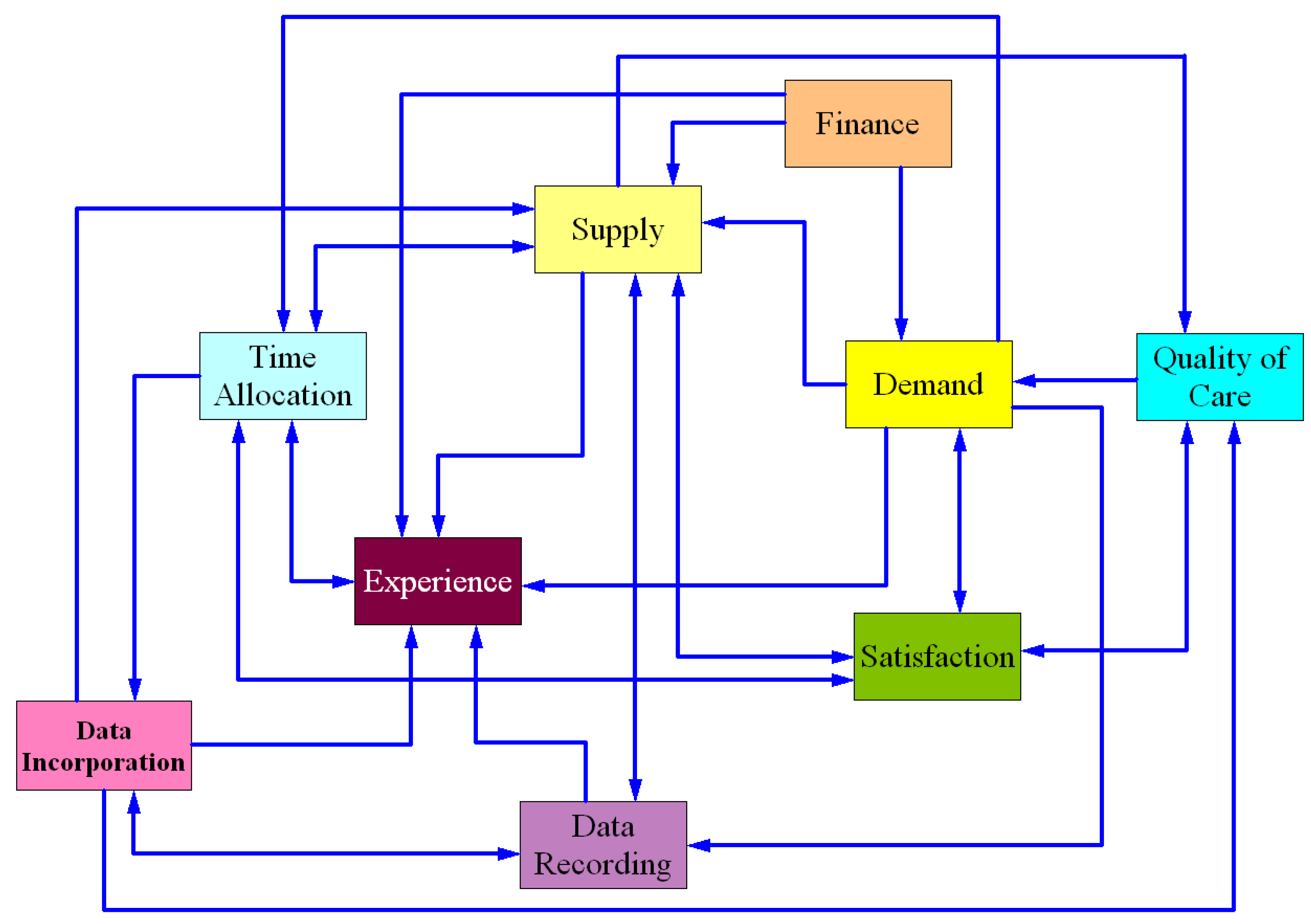
  • Demand calculates the number of patients demanding healthcare services;
  • Supply determines the healthcare service capacity of the organization;
  • Finance is an accounting module calculating costs, revenues, cash balance, and other financial measures;
  • Quality of care accounts for the quality of healthcare services that the organization provides;
  • Satisfaction tracks changes in the satisfaction of patients and healthcare providers;
  • Time allocation includes mechanisms by which physicians allocate their time between three major tasks: medical practice, learning and making use of the electronic health record system, and leisure;
  • Data recording tracks efforts made by physicians and nurses to capture and record digital medical data;
  • Data incorporation represents the level of activities of physicians and nurses in incorporating medical health records in actual medical practice;
  • Experience shows the skill and experience of physicians and nurses in working with the EHR system.
One important goal of the model was to design policies in order to facilitate the EHR implementation processes, and specifically the use of the system by physicians. The original model was used to show that some specific settings were required to streamline the EHR implementation processes. Particularly, different payment systems for physicians were examined to identify effective settings:
  • BASE is the payment system used in the default setting of the model. In this case, physicians are reimbursed based on a capitated payment system.
  • FLEXPAY is a payment system similar to the BASE case, but it also includes an additional bonus for physicians if their satisfaction declines.
  • FIXPAY is a different payment system based on constant salary. In addition, physicians will receive extra bonus pay if their satisfaction declines.
  • FIXPAY2 is also based on constant salary but 20% higher than the FIXPAY case. Additional bonus will be paid to physicians if higher quality of care is observed.
There are seven utility perception equations in the EHR implementation model:
  • physician satisfaction from patient satisfaction,
  • physician satisfaction from leisure,
  • physician satisfaction from income,
  • physician satisfaction from quality of care,
  • patient satisfaction from quality of care,
  • patient satisfaction from wait time, and
  • patient satisfaction from visit time.
Depending on the dynamic state of the system, these variables may vary between −1 and +1; −1 represents extreme disutility, +1 represents extreme utility, and 0 indicates normal (neutral) utility. Each of these utilities then goes through the utility perception processes described in the previous section to yield perceived utility. A binary variable is used to switch between traditional smoothing and peak–end value utility perception formulations.
We should also note that the decision utility formation that was missing from the analysis of the small model is included in this model. The effect of remembered (perceived) utility on decision utility is not well-documented [1,3]. Therefore, this structure is assumed to be as simple as possible and in compliance with the traditional system dynamics method. A smoothing average is used to assume a delay between perceived utility and decision utility which eventually determines decisions of the agents. This is equivalent to the “Delay” process in the perception apparatus of the utility-based decision system in Figure 1. For example, patient satisfaction from wait time will not immediately affect the patients’ decision to stay or leave the system. Even if a patient is unhappy with the wait time, it probably takes her some time to make an active decision based on her remembered utility. Accordingly, the perceived utility—captured by either peak–end or smooth, depending on which model is being tested—is smoothed over time, and only then does it affect the demand for the healthcare system. We expected that this additional structure (delay between remembered and decision utilities) would only moderate the extremity of the peak–end rule and align the overall system behavior towards the traditional (smooth) model. Removal of the new structure (or using a different formulation such as peak–end to capture the difference between remembered and decision utilities) would lead to greater discrepancy between the results of the two (peak–end and smooth) models.
However, preliminary simulation results showed significant discrepancy between outputs of the simple smoothing model and those of the peak–end model. One example of these results is illustrated in Figure 9. While all four graphs show qualitatively different results for the peak–end value formulation than for the standard smoothing formulation, it is the financial balance that shows the implications most drastically. For the smoothing formulation, Financial Balance shows increases with time while the use of the peak–end formulation shows a monotonic decrease in Financial Balance. However, these results were derived from only one possible initial setup of the model, and might not be a good reference for generalization. Indeed, we need a more comprehensive analysis in order to provide a meaningful argument.
We ran 1000 Monte Carlo simulations with multivariate parameter settings. In these simulations, parameters of the model changed in a wide range, as shown in Appendix B, so that the majority of parameter space was covered in the analysis. Each set of Monte Carlo simulations was repeated with a similar random seed on each model (simple smoothing and peak–end) for each payment scenario. Thus, at the end there were 8 (2 models multiplied by 4 payment scenarios) sets of simulations (8000 runs, in total) to be used for comparative analysis.
The EHR implementation process was monitored through the use of four performance parameters: (a) average quality of care; (b) financial balance; (c) average patient wait time; and (d) time spent on EHR.
Comparing all data points for each pair of simulation runs would be a daunting task. Instead, we compared the results at the end of the simulation. In order to take the dynamics of the results into account, averages of the measures were used instead of their final value. This excludes “financial balance”, which itself represents the average of net profit over the simulation period. We compared the results in three different ways: (a) looking for the number of results with significant differences; (b) looking for the number of runs with improved performance in all four performance measures; and (c) number of runs with similar policy implications for both formulations.

3.1. Number of Runs with Significant Difference in Numerical Results between the Two Formulations

The first perspective compares the numerical values of the four performance measures for each of the utility formulations. Here, we compare the simulation runs one by one and count those that generated a significant difference between outputs of the simple smoothing model and those of the peak–end model. Table 1 summarizes the results.
In the first row, we have the percentage of runs with a significant difference in financial balance generated by the simple smoothing model and by the peak–end model. For the base case, 68% of simulation runs generated a discrepancy greater than 10%. This figure changed to 65% upon switching to the FLEXPAY payment system, and to 62% for the FIXPAY scenario. The figures increased to 90% for the FIXPAY2 payment system.
The second row of the table shows the percentage of runs with a significant difference in average quality of care numbers generated by each utility formulation for the different payment systems. For the base case, about 13% of simulation runs for the FLEXPAY and FIXPAY scenarios yielded a significant difference in average quality of care between the two utility perception models (simple smoothing and peak–end). This figure reached about 63% for the FIXPAY2 system.
The third row of Table 1 reports the results for “average patient wait time”. The percentages of simulation runs that generated a difference greater than 10% in this performance measure between the two formulations were about 17%, 11%, 9%, and 33% for the base case, FLEXPAY, FIXPAY, and FIXPAY2, respectively.
The last row of the table shows percentages of simulation runs that generated a significant difference in average EHR usage rate for the two utility formulations. Significant difference here is greater than 1 h. About 10% of simulation runs met that criterion for the first three scenarios. However, 33% of the runs showed a significant difference for the FIXPAY2 scenario.
In summary, the differences in performance measures for the two different utility formulations in the model were significant, especially for the case of FIXPAY2. This implies that for some particular initial settings of the model, it will matter which utility perception formulation is employed. That is, an alternative formulation of utility perception may lead to significantly different results.

3.2. Number of Runs with Improved Performance in All Four Measures for Each Formulation

Now, we take a different look at the problem. This time, we counted the number of simulation runs that created any kind of improvement in all of the four performance measures for each of the different pay policies. More precisely, we first took the simple smoothing model. Then, we compared simulation outputs of the base case with one of the payment systems (e.g., FLEXPAY). Finally, we flagged those runs that showed improvement in all performance measures. We then repeated the comparison between the base case and other payment systems (i.e., FIXPAY and FIXPAY2) and recorded the outcome. The same analysis was conducted for the peak–end model. Results are reported in Table 2.
For the simple smoothing model, FLEXPAY showed improvement in all four parameters in about 29% of the runs, meaning that 29% of simulation runs showed that this payment system could improve financial balance, quality of care, patient wait time, and EHR usage rate. FIXPAY had a lower improvement rate of about 23%. The FIXPAY2 system of payment, however, had a greater improvement rate of about 41%. A policy recommendation based on this model would be inclined towards the use of FIXPAY2 rather than the other two policies.
On the other hand, with the peak–end model, the FLEXPAY payment system showed improvement about 34% of the time. FIXPAY showed improvement about 32% of the time. FIXPAY2 showed improvement in only 7% of the runs. Based on these results, FIXPAY2 is definitely a rejected policy.
While the smoothed utility formulation would recommend the FIXPAY2 policy, the peak–end formulation would likely reject this policy. These conflicting results imply that the selection of utility perception formulation may significantly impact policy recommendations of our models. One might reach dramatically different conclusions if the peak–end model was used over the simple smoothing model.

3.3. Number of Runs with Similar Policy Implications for Both Formulations

For the last perspective, we assessed the likelihood of achieving similar policy outcomes implied by the two utility perception models regardless of capabilities of the policies in improving the system’s behavior. Here, we counted the number of simulations that yielded the same policy implications. To do so, we first took the simple smoothing model and examined the impact of a certain policy (e.g., FLEXPAY) on the performance measures for each single simulation run. As an example, assume that for the simulation run #348 the policy only improved patient wait time (W) and had no positive impact on the other performance measures. Now, we took the same simulation run (#348) for the same policy, but this time with the peak–end formulation. If the results showed improvement in patient wait time (W) and no positive impact on the other performance measures, we could decide that this simulation run generated a “similar” result and would be counted in our stats; otherwise, the simulation run would be discarded. Similarly, any combination of improvement for the simple smoothing formulation had to match with that from the peak–end formulation for the corresponding simulation run to be counted in the “similarity” stats. The results are reported in Table 3.
Similarity rates between the two models are strikingly low. For some policies such as FIXPAY2, there was a 32% chance of achieving similar outcomes from the simple smoothing and the peak–end models. When the FIXPAY policy was applied, the two models yielded more similar outcomes, but even in this case, only 57% of the simulation runs showed similar policy implications.

4. Discussion

System dynamics models tend to use utility considerations in decisions implicitly in the formulation of perceived information or information perception, which is one of the inputs into decisions. Decision utility is defined as the utility based on decisions made, and as such it is an a posteriori quantity. It can be measured, but in modeling, we need to have an a priori formulation that is either a theory or an explicit mental model.
As discussed previously, decision utility is different because the means of utility perception and information perception are different—that is, the way the input arrives to the perception function. Decision utility is also different because it includes psychological factors that may cause bias in the perception of utility—that is, the way in which the input is processed by the perception function. Bias in the perception of information has been articulated in a few system dynamics modeling efforts (see [15] for a recent review), where the only notable alternative perception heuristic has been “anchoring and adjustment” [16,17,18]. Nevertheless, utility perception remains unexplored mainly because most of the time, system dynamics models focus on the producer side of the problem (i.e., the side with a reasonable authority in access to formal data and certain objective analysis capabilities), rather than the consumer side (i.e., the side that often relies on intuitions and feelings to make decisions), where decision utility plays a significant role.
On the consumer side, means of utility perception are fundamentally different from those on the producer side. The information or utility that consumers receive is usually more prone to error or change due to psychological filters. Further, the consumers do not analyze the information as rigorously as the producers do. In the extreme, it is nearly impossible for agents to formally analyze their utilities. The erroneous nature of decision utility formation on the consumer side could lead to a situation where there is a perennial gap between decision utility and experienced utility. Such behavior cannot be reproduced by the traditional smoothing function. Given sufficient adjustment time, the smoothed utility (information) eventually converges to the actual utility (information), while the “real” perceived utility (information)—the utility perceived by the individual as opposed to the perceived utility calculated by the model—may not. Considering the cardinal differences between the two concepts, it should not be surprising that the decision utility formation had a different mechanism than the managerial information perception.
The peak–end rule has been observed in several studies. Two relevant examples are utility from time spent in waiting lines [19] and utility from vacation time (similar to customer satisfaction from a service) [20]. Another relevant setting in which the peak–end rule is successfully tested is the dynamics of labor turnover due to job satisfaction [13]. These are all common dynamic issues being studied extensively in the field of system dynamics. However, the peak–end rule has not been applied in any system dynamics setting. Such an application seems to be a reasonable alternative, at least for policy sensitivity tests in these areas. This situation could be complicated as, decision utility, in contrast to perceived (remembered) utility, can be influenced by time passed, repeated experiences and other psychological factors [21] for which there are no accepted utility perception formulations to date. Despite the lack of consensus in utility formulation, we argue that the possibility of alternative formulations such as the peak–end rule (or others) should be investigated in cases where there is a reason to assume that they might be the dominant decision utility description or as a matter of good practice. These different formulations should be investigated together with a wide parameter space in order to identify potential policy recommendations that differ from those obtained with the traditional information. Much more work needs to be done to understand the effect of alternative utility formulations on the outcomes of system dynamics models, and a good starting point might be the investigation of generic structures and their sensitivity to such formulations.
Our decisions at all levels of aggregation rely on models, be they mental or formal. Hence, it is extremely important to invest in our models. We believe that furthering the exploration of utility perception formulation has significant gains for multiple groups of researchers, including behavioral scientists, economists, system dynamicists, and consequently policy makers. The models or theories developed by the researchers will be used for policy design at some point. Investment in this area will potentially enhance the models, and eventually lead to better policies.
It is usually argued that behavioral sciences (behavioral economics, in particular) could benefit from system dynamics modeling tools [22]. Although not incorrect, we believe that this is not a one-way path. In fact, a continuous dialog must be established between the two fields, as system dynamicists would also benefit from advancements in the field of behavioral sciences. System dynamics modeling practice will be particularly affected by further exploration of the decision utility formulation approaches. As discussed previously, this does not mean that the smoothing practice must be abandoned. Instead, the modeler’s toolbox must upgrade continuously to include a wide variety of modern theories and techniques. Depending on the concept being modeled, the modeler can then pick the assumption that fits better to the problem at hand, whether it is the smoothing, peak–end, or any other construct. Since human decision is the core concept in the system dynamics approach, system dynamics modelers should always be aware of the latest advancements in the field of behavioral and decision sciences. Accordingly, we recommend that alternative formulations for utility perception be included in system dynamics software packages as built-in functions so that applications of theories such as the peak–end rule become readily available to modelers.
This paper paves the way for the implementation of all the aforementioned suggestions. It builds a basis for further testing of the peak–end rule (or similar behavioral rules) in system dynamics settings. For future studies, we suggest that the peak–end rule be examined on more system dynamics models to see whether or not the implications hold true. It would also be interesting to test human decision rules in experimental settings such as simulation games where the player decisions are tracked and compared with expected behaviors of the peak–end rule or smoothing. Further, we encourage exploration of other decision utility heuristics. They could be translated into system dynamics and tested for potential impact on policy outcomes. Finally, we did not consider the impact of the input quality on dynamics of decisions. In fact, system dynamics models rarely distinguish between high and low qualities of information inputs to decision functions. A framework that allows such considerations, such as Brunswik’s lens model [23], might open some new venues in system dynamics modeling and research.

5. Conclusions

In this paper, we apply a decision utility formulation to two system dynamics models and compare the results to those obtained from traditional perceived information formulations. Specifically, we use the peak–end rule for comparison with the exponential smoothing formulation. This rule, a result from behavioral sciences, has been used successfully to describe preferences in a range of applications.
Experiments with a simple theoretical model that focuses on the different utility formulations revealed significant differences in model outcomes. The same model was replicated for 1000 agents and simulated for 1000 different initial settings to make sure that (a) the peak–end rule at the individual level manifests itself at the population (aggregate) level as well; and that (b) results remain robust under different random inputs.
The peak–end rule was also applied in a medium-size model of electronic health record (EHR) implementation. The EHR model has many (positive and negative) feedback loops, and includes seven utility perception equations and four different payment schemes. One thousand Monte Carlo simulation runs were performed for each formulation and for each of the four payment policies, yielding 8000 total runs. Comparison between simulation runs across different models and different scenarios revealed that discrepancy in outputs of different models was considerable. The magnitude of the discrepancy, however, depended on the initial setup of the models. Results also showed that it is very likely that the two models would lead to diametrically opposed policy recommendations.
Based on these results, we conclude that different formulations for utility perception actually matter. The point of this investigation was not to prove that the peak–end rule was necessarily the better formulation for the EHR model or any other model. Rather, we argue that the formulation of the decision utility for preferences is likely to affect recommended policies.

Supplementary Materials

The models presented in this article (including all the equations and parameters) are available online at https://www.mdpi.com/2079-8954/6/4/37/s1.

Author Contributions

S.P.L. and I.B.-O. conceived and designed the experiments and wrote the paper; S.P.L. performed the experiments and analyzed the data.

Funding

This research received no external funding.

Conflicts of Interest

The authors declare no conflict of interest.

Abbreviation

The following abbreviation is used in this manuscript:
EHR:Electronic Health Records

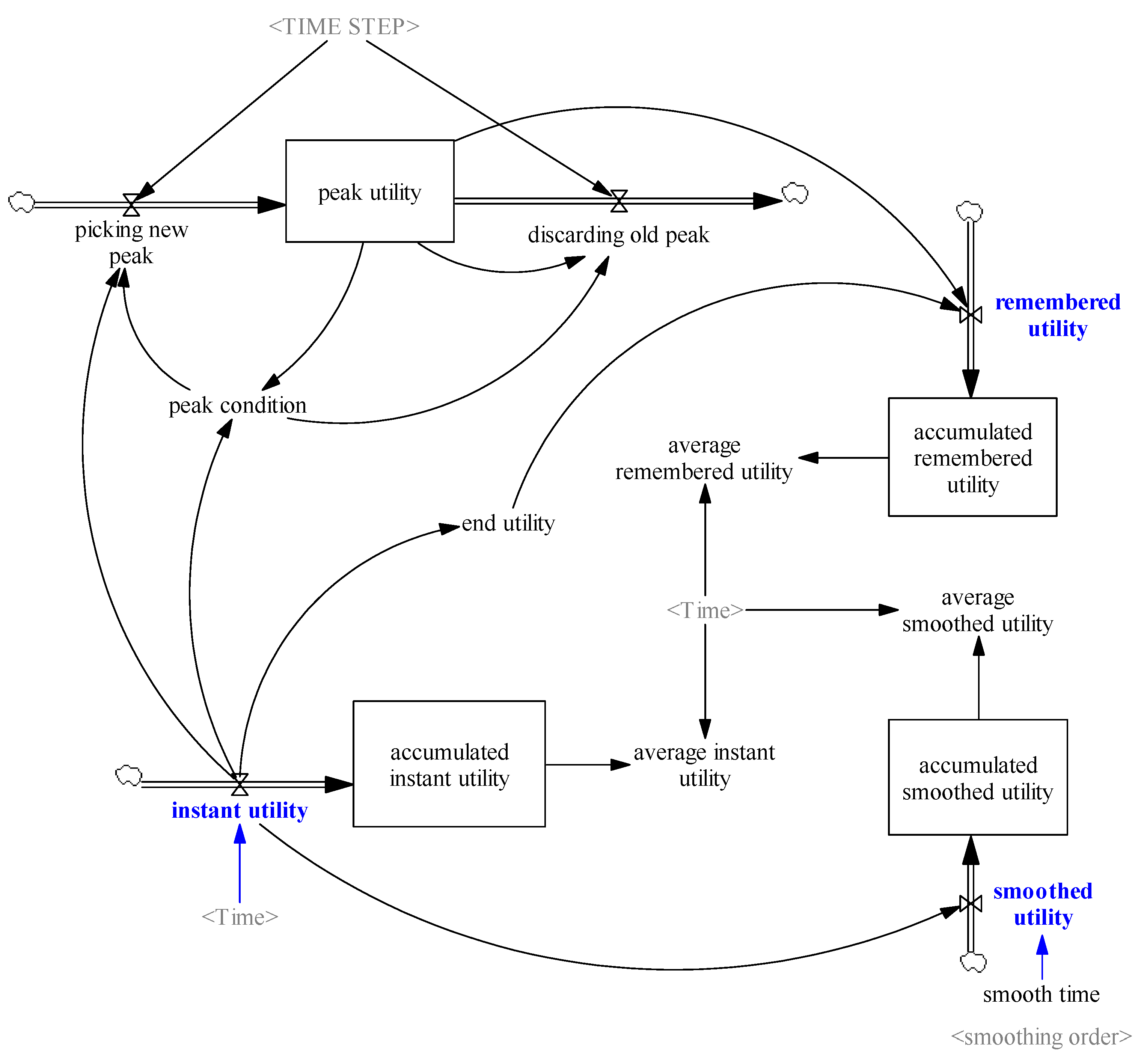
Appendix A. Equations of the Peak–End Module

accumulated instant utility = INTEG (instant utility,0)
Units: Dmnl
 
accumulated remembered utility = INTEG (remembered utility,0)
Units: Dmnl
 
accumulated smoothed utility = INTEG (smoothed utility,0)
Units: Dmnl
 
average instant utility = accumulated instant utility / Time
Units: 1 / Week
 
average remembered utility = accumulated remembered utility / Time
Units: 1 / Week
 
average smoothed utility = accumulated smoothed utility / Time
Units: 1 / Week
 
discarding old peak = peak utility * peak condition / TIME STEP
Units: 1 / Week^2
 
end utility = instant utility
Units: 1/ Week
 
instant utility = SIN(Time * max utility) * RANDOM UNIFORM(0, 1, random seed)
Units: 1 / Week
 
max utility = 1
Units: 1 / Week
 
random seed = 1
Units: Dmnl
 
peak condition =
IF THEN ELSE(ABS(instant utility) >= ABS(peak utility), 1, 0)
Units: Dmnl
 
peak utility = INTEG (picking new peak-discarding old peak,0)
Units: 1 / Week
 
picking new peak = peak condition * instant utility / TIME STEP
Units: 1 / Week^2
 
remembered utility = (end utility + peak utility) / 2
Units: 1 / Week
 
smooth time = 2
Units: Week
 
smoothed utility =
SMOOTH N(instant utility, smooth time, 0, smoothing order)
Units: 1 / Week
 
smoothing order = 1
Units: Dmnl
 
TIME STEP = 0.0078125
Units: Week

Appendix B. EHR Model’s Parameter Variation Range

PBPI=RANDOM_UNIFORM(0.00001,0.1)
PBPI --- Productivity booster per unit of investment (1 / $)
 
PCR=RANDOM_UNIFORM(0.1,0.9)
PCR --- Contact rate: indicates how frequently (potential and
 /or current) patients meet each other (1 / Week)
 
PEHQ=RANDOM_UNIFORM(0,1)
PEHQ --- Elasticity of quality of care in response to physician
 satisfaction (Dmnl)
 
PEHRMC=RANDOM_UNIFORM(0.00001,0.01)
PEHRMC --- Unit cost of EHR maintenance ($ / (Week * Record))
 
PEIHS=RANDOM_UNIFORM(0,1)
PEIHS --- Elasticity of physician satisfaction in response to
 physician income (Dmnl)
 
PELHS=RANDOM_UNIFORM(0,1)
PELHS --- Elasticity of physician satisfaction in response to
 physician leisure time (Dmnl)
 
PEQDI=RANDOM_UNIFORM(0,1)
PEQDI --- Elasticity of quality of care in response to effective
 usage of EHR (Dmnl)
 
PEQHS=RANDOM_UNIFORM(0,1)
PEQHS --- Elasticity of physician satisfaction in response to
 quality of care (Dmnl)
 
PEQPS=RANDOM_UNIFORM(0,1)
PEQPS --- Elasticity of patient satisfaction in response to
 quality of care (Dmnl)
 
PEQT=RANDOM_UNIFORM(0,1)
PEQT --- Elasticity of quality of care in response to average
 amount time a physician spends on a patient visit (Dmnl)
 
PESHS=RANDOM_UNIFORM(0,1)
PESHS --- Elasticity of physician satisfaction in response to
 patient satisfaction (Dmnl)
 
PETPS=RANDOM_UNIFORM(0,1)
PETPS --- Elasticity of patient satisfaction in response to time
 spent per patient (Dmnl)
 
PEWPS=RANDOM_UNIFORM(0,1)
PEWPS --- Elasticity of patient satisfaction in response to
 patient wait time (Dmnl)
 
PEXMC=RANDOM_UNIFORM(0,1)
PEXMC --- Exogenous management commitment to EHR implementation
 (Dmnl)
 
PFC=RANDOM_UNIFORM(10,000, 1,000,000)
PFC --- Fixed costs ($ / Week)
 
PFINC=RANDOM_UNIFORM(5,20)
PFINC --- Normal financial coverage time (Week)
 
PMCPD=RANDOM_UNIFORM(0.0001,0.01)
PMCPD --- Supply cost of paper data records ($ / Record)
 
PMEXP=RANDOM_UNIFORM(100,000, 1,600,000)
PMEXP --- Initial (normal) marketing expenditure ($ / Week)
 
PMP=RANDOM_UNIFORM(1000, 100,000)
PMP --- Normal malpractice premium rate ($ / People)
 
PPB=RANDOM_UNIFORM(20,000, 400,000)
PPB --- Maximum productivity booster investment per physician
 ($ / (People * Week))
 
PPHE=RANDOM_UNIFORM(100,1000)
PPHE --- Normal physian experience in using EHR (Hour / People)
 
PSCPV=RANDOM_UNIFORM(100,1000)
PSCPV --- Normal medical supply cost per patient visit
 ($ / People)
 
PTCPD=RANDOM_UNIFORM(0.05,0.2)
PTCPD --- Normal time a physician needs to capture and record a
 patient’s data (Hour /People)
 
PTIPD=RANDOM_UNIFORM(0.05,0.2)
PTIPD --- Normal time an average physician needs to incorporate
 a patient’s data into practice (Hour / People)
 
TAC=RANDOM_UNIFORM(6,24)
TAC --- Cost averaging time (Week)
 
TATSP=RANDOM_UNIFORM(2,8)
TATSP --- Time delay to adjust time spent per patient (Week)
 
TBD=RANDOM_UNIFORM(20,80)
TBD --- Productivity booster decay time (Week)
 
TEDI=RANDOM_UNIFORM(0.5,2)
TEDI --- Time delay for data incorporation to become effective
 (Week)
 
TEID=RANDOM_UNIFORM(5,20)
TEID --- Experience internalization delay (Week)
 
TENVP=RANDOM_UNIFORM(5,20)
TENVP --- Time delay to educate nurses for participating in
 patient visits (Week)
 
TEXMC=RANDOM_UNIFORM(10,200)
TEXMC --- Duration of exogenous management commitment to EHR
 implementation (Week)
 
TF=RANDOM_UNIFORM(2,20)
TF --- Time delay for financial state to affect expenditure
 (Week)
 
TFE=RANDOM_UNIFORM(50,200)
TFE --- Time constant to forget EHR experience and skills (Week)
 
TIMEP=RANDOM_UNIFORM(5,20)
TIMEP --- Perception time delay (Week)
 
TME=RANDOM_UNIFORM(10,40)
TME --- Time delay for marketing to become effective (Week)
 
TNV=RANDOM_UNIFORM(2,10)
TNV --- Time delay for nurses to be ready for help in patient
 visit (Week)
 
TPDL=RANDOM_UNIFORM(2000,4000)
TPDL --- Paper data life time (Week)
 
TREP=RANDOM_UNIFORM(5,20)
TREP --- Time for reputation to evolve (Week)
 
TSS=RANDOM_UNIFORM(5,20)
TSS --- Time constant to smooth satisfaction (Week)
 
TTA=RANDOM_UNIFORM(2,8)
TTA --- Time delay to reallocate personal time (Week)
 
TWA=RANDOM_UNIFORM(5,20)
TWA --- Time delay to adjust wage rates (Week)
 
PPSW=RANDOM_UNIFORM(0,5)
PPSW --- Parameter affecting shape of the function FIPSW
 [Paitient satisfaction from wait time] (Dmnl)
 
PPST=RANDOM_UNIFORM(0,5)
PPST --- Parameter affecting shape of the function FIPST
 [Paitient satisfaction from visit time] (Dmnl)
 
PPSQ=RANDOM_UNIFORM(0,5)
PPSQ --- Parameter affecting shape of the function FIPSQ
 [Patient satisfaction from quality of care] (Dmnl)
 
PHSQ=RANDOM_UNIFORM(0,5)
PHSQ --- Parameter affecting shape of the function FIHSQ
 [Physician satisfaction from quality of care] (Dmnl)
 
PHSL=RANDOM_UNIFORM(5,15)
PHSL --- Parameter affecting shape of the function FIHSL
 [Physician satisfaction from leisure] (Dmnl)
 
PHSI=RANDOM_UNIFORM(0,5)
PHSI --- Parameter affecting shape of the function FIHSI
 [Physician satisfaction from income] (Dmnl)
 
PHSP=RANDOM_UNIFORM(0,5)
PHSP --- Parameter affecting shape of the function FIHSP
 [Physician satisfaction from patient satisfaction] (Dmnl)
 
TPR=RANDOM_UNIFORM(30,100)
TPR --- Time delay for patients to return to the system (Week)
 
PEPB=RANDOM_UNIFORM(0.01,0.5)
PEPB --- Productivity elasticity of productivity booster (Dmnl)
 
TPHA=RANDOM_UNIFORM(5,20)
TPHA --- Normal time delay to hire (fire) physicians (Week)
 
TSDS=RANDOM_UNIFORM(1,4)
TSDS --- Time to smooth desired number of staff (Week)

References

  1. Kahneman, D.; Wakker, P.P.; Sarin, R. Back to Bentham? Explorations of Experienced Utility. Q. J. Econ. 1997, 112, 375–405. [Google Scholar] [CrossRef] [Green Version]
  2. Kahneman, D. Experienced utility and objective happiness: A moment-based approach. Psychol. Econ. Decis. 2003, 1, 187–208. [Google Scholar]
  3. Kahneman, D.; Thaler, R.H. Anomalies: Utility Maximization and Experienced Utility. J. Econ. Perspect. 2006, 20, 221–234. [Google Scholar] [CrossRef] [Green Version]
  4. Samuelson, P.A. Consumption Theory in Terms of Revealed Preference. Economica 1948, 15, 243–253. [Google Scholar] [CrossRef]
  5. Fredrickson, B.L.; Kahneman, D. Duration neglect in retrospective evaluations of affective episodes. J. Personal. Soc. Psychol. 1993, 65, 45. [Google Scholar] [CrossRef]
  6. Kahneman, D.; Fredrickson, B.L.; Schreiber, C.A.; Redelmeier, D.A. When More Pain Is Preferred to Less: Adding a Better End. Psychol. Sci. 1993, 4, 401–405. [Google Scholar] [CrossRef]
  7. Redelmeier, D.A.; Kahneman, D. Patients’ memories of painful medical treatments: Real-time and retrospective evaluations of two minimally invasive procedures. Pain 1996, 66, 3–8. [Google Scholar] [CrossRef]
  8. Forrester, J.W. Market Growth as Influenced by Capital Investment. Ind. Manag. Rev. 1968, 9, 83. [Google Scholar]
  9. Gigerenzer, G.; Gaissmaier, W. Heuristic Decision Making. Annu. Rev. Psychol. 2011, 62, 451–482. [Google Scholar] [CrossRef] [PubMed] [Green Version]
  10. Evans, J.S.B.T. Dual-Processing Accounts of Reasoning, Judgment, and Social Cognition. Annu. Rev. Psychol. 2008, 59, 255–278. [Google Scholar] [CrossRef] [PubMed]
  11. Stone, A.A.; Broderick, J.E.; Kaell, A.T.; DelesPaul, P.A.E.G.; Porter, L.E. Does the peak-end phenomenon observed in laboratory pain studies apply to real-world pain in rheumatoid arthritics? J. Pain 2000, 1, 212–217. [Google Scholar] [CrossRef] [PubMed]
  12. Langer, T.; Sarin, R.; Weber, M. The retrospective evaluation of payment sequences: Duration neglect and peak-and-end effects. J. Econ. Behav. Organ. 2005, 58, 157–175. [Google Scholar] [CrossRef]
  13. Clark, A.E.; Georgellis, Y. Kahneman meets the quitters: Peak-end behaviour in the labour market. In Proceedings of the BHPS-2007 Conference, Colchester, UK, 5–7 July 2007. [Google Scholar]
  14. Langarudi, S.P.; Strong, D.M.; Saeed, K.; Johnson, S.A.; Tulu, B.; Trudel, J.; Volkoff, O.; Pelletier, L.R.; Lawrence, G.; Bar-On, I. Dynamics of EHR Implementations. In Proceedings of the 32nd International Conference of the System Dynamics Society, Delft, The Netherlands, 20–24 July 2014; p. 30. [Google Scholar]
  15. Morrison, J.B.; Oliva, R. Integration of Behavioral and Operational Elements Through System Dynamics. In The Handbook of Behavioral Operations; Wiley: New York, NY, USA, 2017. [Google Scholar]
  16. Tversky, A.; Kahneman, D. Judgment under Uncertainty: Heuristics and Biases. Science 1974, 185, 1124–1131. [Google Scholar] [CrossRef] [PubMed]
  17. Kahneman, D.; Slovic, P.; Tversky, A. Judgment under Uncertainty: Heuristics and Biases; Cambridge University Press: New York, NY, USA, 1982. [Google Scholar]
  18. Jacowitz, K.E.; Kahneman, D. Measures of Anchoring in Estimation Tasks. Personal. Soc. Psychol. Bull. 1995, 21, 1161–1166. [Google Scholar] [CrossRef]
  19. Carmon, Z.; Kahneman, D. The Experienced Utility of Queuing: Real Time Affect and Retrospective Evaluations of Simulated Queues; Duke University: Durham, NC, USA, 1996. [Google Scholar]
  20. Kemp, S.; Burt, C.D.B.; Furneaux, L. A test of the peak-end rule with extended autobiographical events. Mem. Cogn. 2008, 36, 132–138. [Google Scholar] [CrossRef] [Green Version]
  21. Miron-Shatz, T. Evaluating multiepisode events: Boundary conditions for the peak-end rule. Emotion 2009, 9, 206–213. [Google Scholar] [CrossRef] [PubMed]
  22. Bahaddin, B.; Weinberg, S.; Luna-Reyes, L.; Andersen, D. Simulating Lifetime Saving Decisions: The Behavioral Economics of Countervailing Cognitive Biases. In Proceedings of the 35th International Conference of the System Dynamics Society, Cambridge, MA, USA, 16–20 July 2017; p. 21. [Google Scholar]
  23. Brunswik, E. Perception and the Representative Design of Psychological Experiments, 2nd ed.; University of California Press: Berkeley, CA, USA, 1956. [Google Scholar]
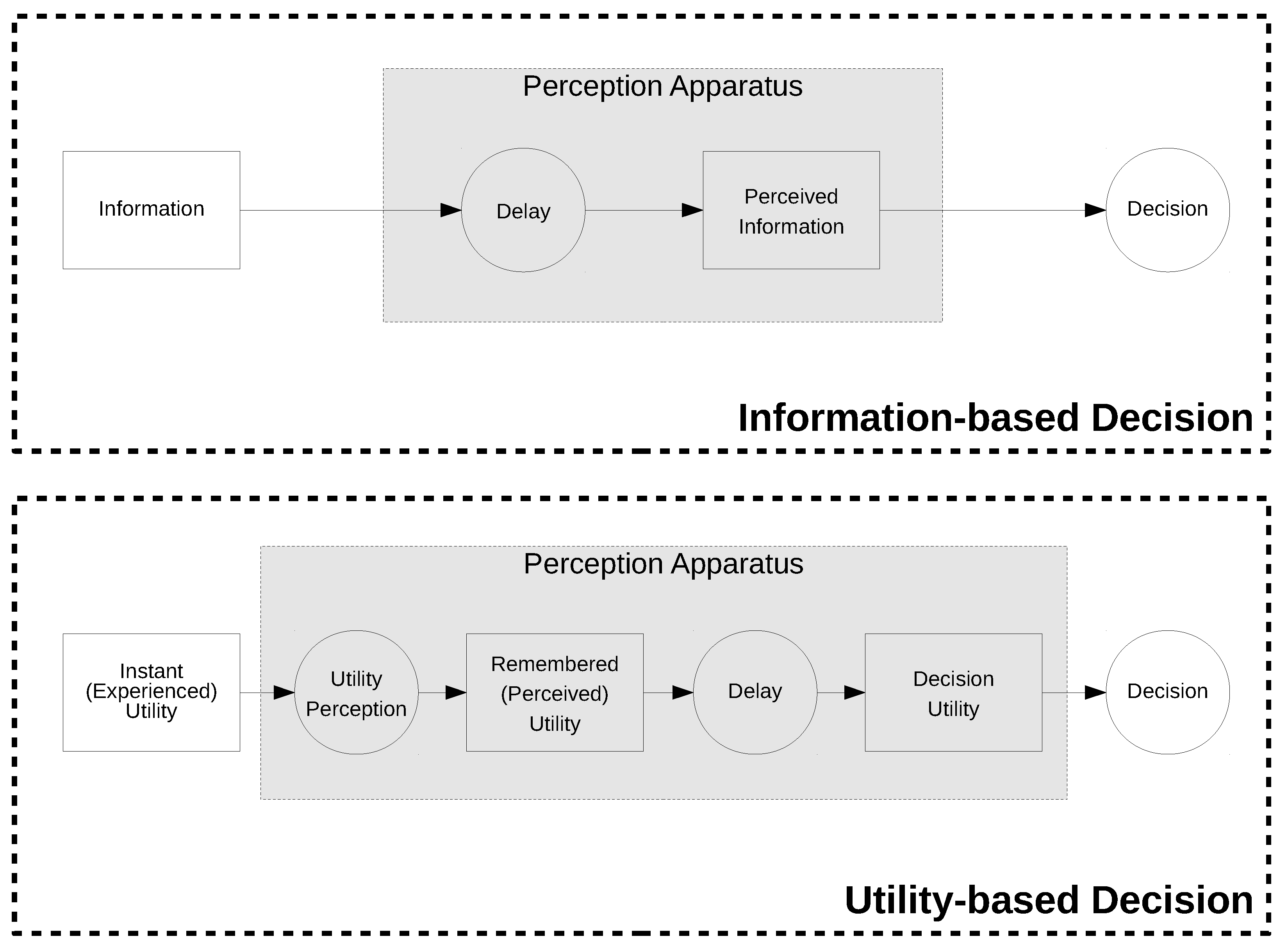
1
Please note that the customers’ perception of satisfaction (utility) is not discussed explicitly in the market growth model. In the original model, x is delivery delay, and x ¯ is the perceived delivery delay. The latter is then used directly to calculate demand. In other words, the mechanism through which the customers gain utility due to changes in delivery time, and subsequently adjust their demand, is encapsulated in the formulation of x ¯ . In an attempt to make the utility consideration explicit, we refer to this formulation as “utility perception”.
2
A generally used rule states that the simulation time step ( d t ) must be smaller than 25% of the smallest time constant in the model in order to avoid integration errors, and at the same time, to achieve reasonable precision for the simulation. As a result, the ratio of d t T will always be smaller than 0.25 .
3
Recent advancements in the field of behavioral sciences suggest a few variants for decision heuristics as presented by Gigerenzer and Gaissmaier [9]. For example, dual-process theories provide an explanation for how individuals make decisions and how such processes could lead to a bias in decision-making [10]. Due to limited resources, we were unable to examine all these alternatives in a system dynamics setting. However, the interested reader is encouraged to further explore this research area.
4
It is noteworthy that we also examined different forms of test inputs (including pink noise) on the model. Results of these alternative tests are not reported here, but the implication remains the same as presented.
5
The default random seed of the Vensim model was 1; To produce the alternative experiment, Vensim’s random seed of 123 was used.
6
Note that the current analysis assumes no interactions between the agents, although we believe that the agent interactions could lead to more extreme instances, thus augmenting the peak–end manifestation even further (e.g., through word-of-mouth).
Figure 1. A framework to compare information-based vs. utility-based decision mechanisms.
Systems 06 00037 g001
Figure 2. Structure of a simple example of utility perception.
Systems 06 00037 g002
Figure 3. Behavior of the system in response to irregular oscillatory instant utility.
Systems 06 00037 g003
Figure 4. Change in peak utility in response to irregular oscillatory instant utility.
Systems 06 00037 g004
Figure 5. Behavior of the system in response to alternative irregular oscillatory instant utility.
Systems 06 00037 g005
Figure 6. Change in peak utility in response to alternative irregular oscillatory instant utility.
Systems 06 00037 g006
Figure 7. Propagation of individual peak–end behavior to the societal level.
Systems 06 00037 g007
Figure 8. Sector view of the electronic health records (EHR) implementation model [14].
Systems 06 00037 g008
Figure 9. Comparison between simulation outputs of the simple smoothing model and the peak–end model.
Systems 06 00037 g009
Table 1. Number of runs with significant difference in results between the two formulations for each payment system.
CriterionBASEFLEXPAYFIXPAYFIXPAY2
| B v B s | > 10 % 68.1%65.2%61.9%89.9%
| Q v Q s | > 10 % 13.3%13.6%12.7%62.6%
| W v W s | > 10 % 16.6%10.9%8.7%48.0%
| T v T s | > 1 h9.1%11.4%9.7%33.1%
B = financial balance at the end of simulation; Q = average quality of care; W = average patient wait time; T = average physician time spent on EHR; v = index representing PEAK–END VALUE formulation; s = index representing SIMPLE SMOOTHING formulation.
Table 2. Number of runs with improved performance in all four parameters for each formulation.
Utility Perception MethodFLEXPAYFIXPAYFIXPAY2
Simple Smoothing Model28.9%23.4%41.3%
Peak–End Value Model33.6%31.9%6.9%
Table 3. Number of runs with similar policy implications for both formulations.
Payment SystemFLEXPAYFIXPAYFIXPAY2
Similarity rate55.5%57.1%31.6%

