Consideration of Wind Speed Variability in Creating a Regional Aggregate Wind Power Time Series

Abstract

For the purposes of understanding the impacts on the electricity network, estimates of hourly aggregate wind power generation for a region are required. However, the availability of wind production data for the UK is limited, and studies often rely on measured wind speeds from a network of meteorological (met) stations. Another option is to use historical wind speeds from a reanalysis dataset, with a resolution of around 40–50 km. Mesoscale models offer a potentially more desirable solution, with a homogeneous set of wind speeds covering a wide area at resolutions of 1–50 km, but they are computationally expensive to run at high resolution. An understanding of the most appropriate choice of data requires knowledge of the variability in time and space and how well that is represented by the choice of model. Here it is demonstrated that in regions offshore, or in relatively smooth terrain where variability in wind speeds is smaller, lower resolution models or single point records may suffice to represent aggregate power generation in a sub-region. The need for high resolution modelling in areas of complex terrain where spatial and temporal variability is higher is emphasised, particularly when the distribution of wind generation capacity is uneven over the region.

1. Introduction

The connection of large amounts of wind generation to the electricity network is frequently discussed, often focusing on aspects of the variability of wind power and the difficulty in managing less-predictable power flows. Developing a model to determine the impact of power fluctuations is crucial for electricity network operators.

For a specific region of interest, the combined effects of spatial and temporal variability will affect its aggregate power production. The wind climate in the UK is affected strongly by heterogeneous terrain, leading to diverse wind speeds within relatively small areas. Wind generation capacity is not evenly distributed around the country, due to this variability, but also grid capacity, planning constraints, land availability and the different regulations and incentives provided by local governments. Temporally, different weather systems affecting different parts of the country could smooth the aggregate output, but equally, when the weather is similar everywhere, the peaks and troughs will be emphasised.

The availability of suitable data to analyse the variability characteristics of UK wind generation is limited. Actual metered power is protected by commercial interests, whilst market data can be hard to process and both can be corrupted by undocumented reliability issues. The pace of wind generation development is such that only a few years of representative data would be available. Many previous studies have used some variation of a method involving transforming met station data to wind turbine hub height, applying a turbine power curve and aggregating this for a region. Sinden [1] used wind speeds measured at 10m above ground level (a.g.l) at 66 unspecified met stations over a period of 23 years and, using a wind turbine power curve, derived an annual capacity factor for each record. Wind speeds were adjusted according to their situation (coastal, inland or island) and region (south, central or north) so that the annual capacity factor for the region was considered appropriate, and the overall capacity factor for the UK would be 30%. Offshore sites were not considered, and the capacity was considered to be evenly distributed at the met station locations.

In the context of analysing surface wind speed variability more generally, Earl et al. [2] describe wind power variability with a similar method to [1] using 10 m wind speed data from 40 UK met stations. As with [1], this work assumes the distribution of wind capacity matches the distribution of met stations—an assumption that could be misleading, as will be shown later. This does not detract from their overall conclusion that historical interannual variability of wind speeds is relatively large.

Pöyry [3] present an analysis of aggregate power variability, which again uses met station data measured at 10 m a.g.l, in this case over 8 years from 35 onshore locations around Britain and Ireland. Offshore is considered using reanalysis model points. The sites were chosen to be representative of areas likely to see future development but their locations are not identified explicitly, nor the capacity scenario for each area. The authors state that it is not possible to verify the hourly GB output due to lack of data, but for the year 2007, a good correlation of the model data is shown for metered hourly Irish capacity factors.

Met station datasets often have some periods with no records, and have limited coverage, particularly offshore. One option for addressing this involves creating a statistical time series model of aggregate power, such as that described in [4]. The model has been trained on a set of met station records, transformed into a single variable representing UK power output. The training dataset consisted of 6 years of wind speeds at 10 m a.g.l from 116 onshore met stations. The power for each of 16 regions was taken as the average power from all the stations in that region and the capacity in each region weighted according to a generation scenario proposed for 2030. A relatively simple adjustment was made to allow for the inclusion of offshore sites which typically have some different time series characteristics.

An investigation by Kubik et al. [5] established a basis for using relatively low resolution reanalysis data (~50 km) as an alternative to met station datasets to derive regional aggregate power estimates. Good correspondence was found between actual power outputs and their estimate from the MERRA reanalysis [6] for Northern Ireland, but the authors note that the wind capacity and the met stations used in the comparison are quite evenly distributed across the study region. Reid and Turner [7] also compared the relationships between mesoscale model wind speed output (at 40 km resolution) and observations, concluding that observations averaged over the model grid cell matched the model output more closely than each individual station within the cell, due to the inability of the model to capture the sub-grid-scale features present in the wind climate at each station. The model and the aggregate observations had high correlation coefficients, indicating similar co-variability.

A mesoscale model has the advantage of covering the studied region at a reasonably high spatial and temporal resolution for a defined period of time. The study in [8] presents the results of an hourly 11-year hindcast of such a model WRF (Weather Research and Forecasting) [9], at 3 km resolution, where the wind speeds from the closest model level above ground were interpolated to the required hub height of a wind turbine and converted using the known capacity and type of wind turbine in use at the actual sites of all existing, planned or under-construction wind farms in the UK. The aggregate GB load factor was computed and adjusted based on actual load factors measured via the ROC (Renewables Obligation Certificate) register for a short validation period. Because this analysis applies wind farm capacities in their true locations, and the WRF model can provide validated wind speeds over the entire UK area, it can potentially represent the hourly wind generation capacity factor more closely. It is, however, limited to 11 years, which will not capture any inter-decadal variability in wind climate.

Clearly, the higher the resolution of the mesoscale model used, the more representative its output is likely to be of the local wind climate at any point within a model grid cell, but equally, higher resolutions and longer time series require large computational resources to run, store and access. The ability of WRF to capture regional variability in areas of complex terrain in Spain has been studied in [10]. It was found that compared to a dense network of observations (35 stations in total) over a region of around 1.5° × 1.5° latitude/longitude, the daily variability in a 2 km resolution WRF simulation was reasonably similar, but with some differences. The differences were particularly evident in the zonal flow (i.e., west-east), which in this area is more strongly affected by local topographical features. The authors judged it successful enough to use the WRF simulation as a baseline to identify that a smaller number of measuring stations would be sufficient to capture the spatial variability characteristics in the region in question.

The following work starts from an assumption that using a high resolution mesoscale model like WRF, in general, offers the most appropriate way to estimate UK aggregate wind generation. The study identifies situations where more accessible, less expensive methods such as lower resolution reanalysis products or met stations may offer comparable representation of variability for a region and where, indeed, WRF at the resolution available here may not itself be adequate. The variability characteristics of the UK wind climate are first characterised spatially and temporally using the WRF wind speeds as described in [11]. The requirement for additional, higher resolution modelling in some areas is indicated, and conversely, also those areas where lower resolution model or lower density met station records would suffice. A model is created to compare the characteristics of wind power production as derived from single point measurements, lower resolution models and the full-resolution WRF analyses in sub-regions with existing wind generation capacity.

2. Methodology

The work is divided into three sections. Firstly, the spatial and temporal patterns of 10m wind speed variability across the country are examined with reference to how spatial averaging or aggregation might affect results. Secondly, the specific effects of spatial resolution on hourly variability are considered. Thirdly, this is discussed in light of the impact of wind variability on the electricity network and how representative wind power generation data for the purposes of network studies might best be achieved.

The WRF (Weather Research and Forecast) Model provides 11 years of hindcast wind speed data (2000–2010) at 3 km spatial resolution over the UK and surrounding onshore waters. The model run has been thoroughly validated in [11]. A summary of the error statistics compared with various sets of historical data is given in [8] and indicates that the model matches very closely with onshore met station records, with some (consistent) bias evident in offshore areas.

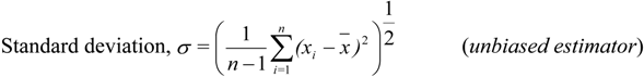
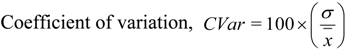
A key measure of variability for studies involving electricity network integration is how much the output would vary from a given mean baseline. As shown in [12], the dimensionless coefficient of variation (CVar) is calculated as the ratio of the standard deviation to the mean (presented as a percentage). This is shown in Equations (1)–(3) (assuming a normal distribution), where n is the number of samples in the dataset.

(1)

(2)

(3)

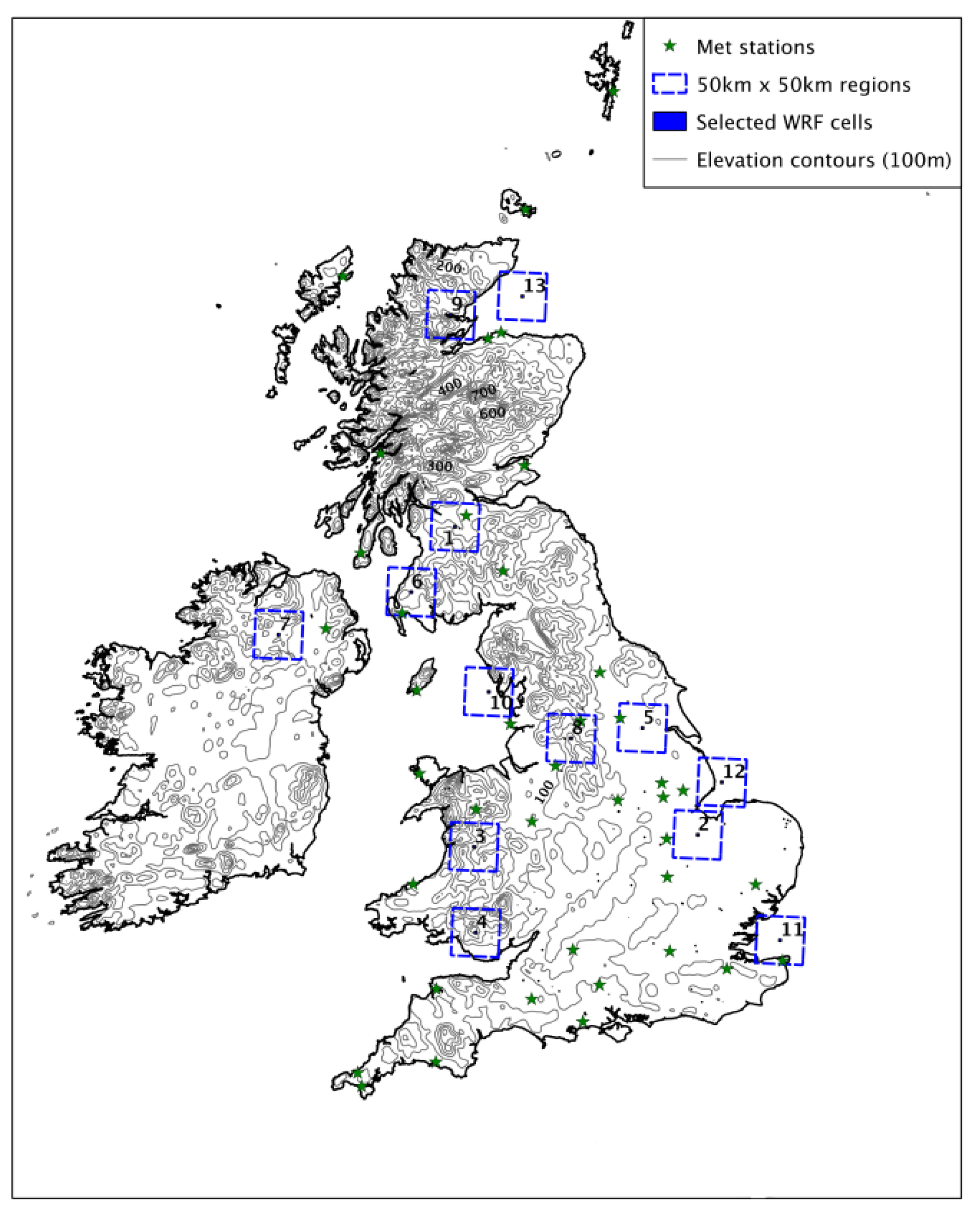
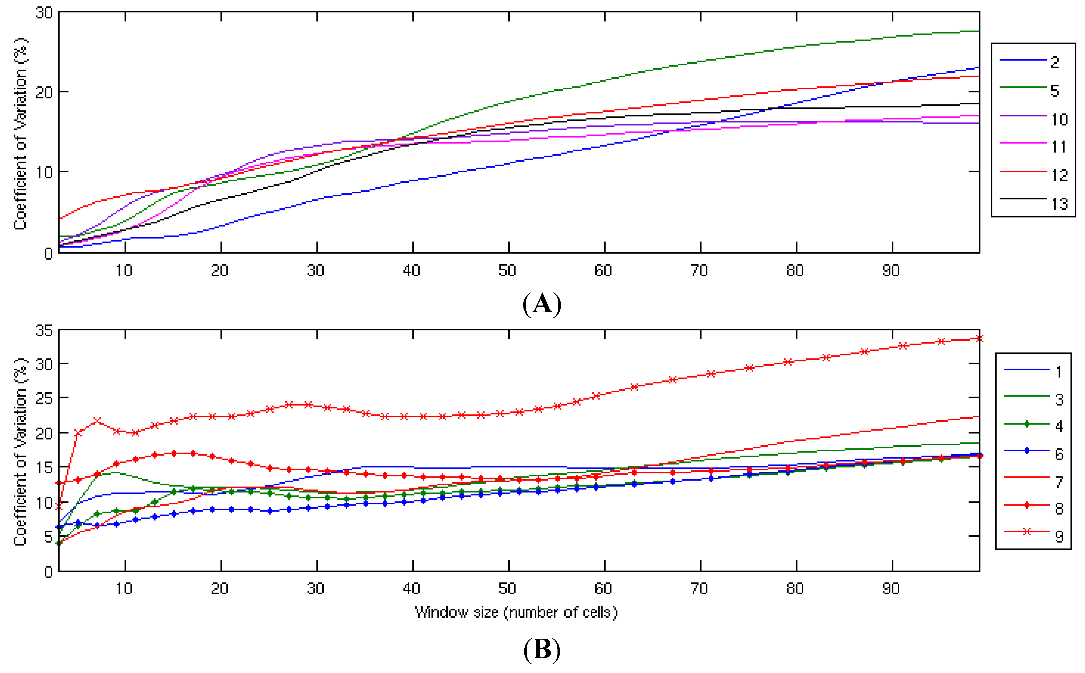
The interannual variability of 10 m and 80 m wind speed is calculated for each grid cell, where the samples, x_i, are the yearly means, x the long-term mean, and n = 11 (number of years). For the consideration of the spatial variability of the long-term mean wind speed, a method similar to that used in [12] is applied. For a given number of cells, n, around the central cell in question, the standard deviation is calculated as in equation 2, where the mean, x , is taken to be the long-term (11-year) mean of the central cell and x_i is the long-term mean of each of the surrounding cells.

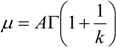
Applying the calculation of coefficient of variation to hourly wind speed data requires a modified approach. Whilst the interannual variability may be suitably described by a normal distribution, hourly observed values have been shown in, for example, [13] to be typically Weibull distributed, rather than normal. The mean, μ, and standard deviation, σ, in this case are calculated from the fitted Weibull shape and scale parameters, A and k, as:

(4)

(5)

The coefficient of variation is then the ratio of the standard deviation to the mean, as in Equation (3).

Hypothetical wind capacity factors are derived for the WRF cells using the hourly 80 m wind speeds combined with a generic aggregate power curve, representative of multiple wind turbines in a single location, rather than an individual wind turbine power curve (as described in [11], data from [14]). The wind generation capacity statistics for the UK, along with the locations of the generators, has been obtained from [15] and has been used along with the derived capacity factors for each cell to produce aggregate power output.

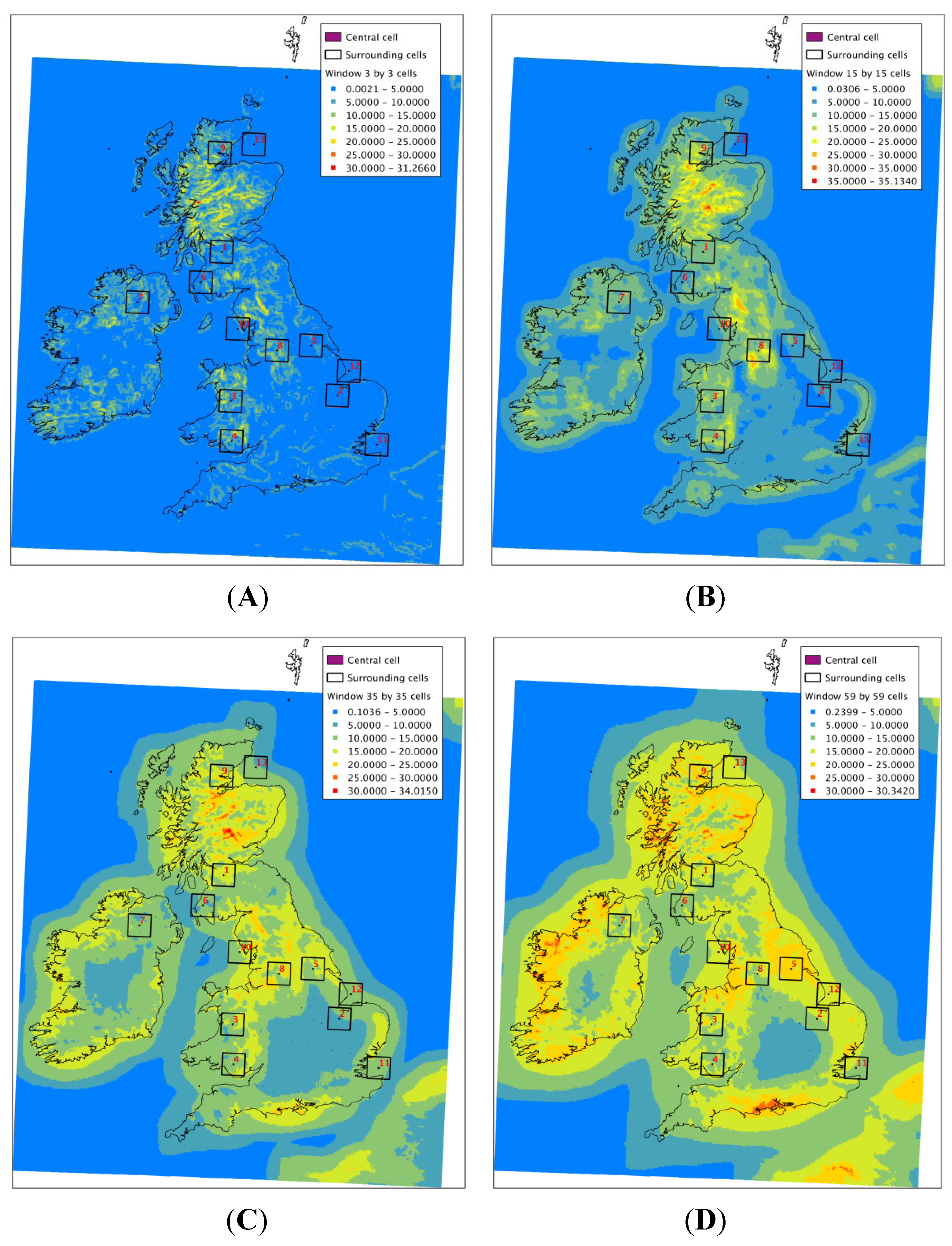
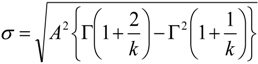
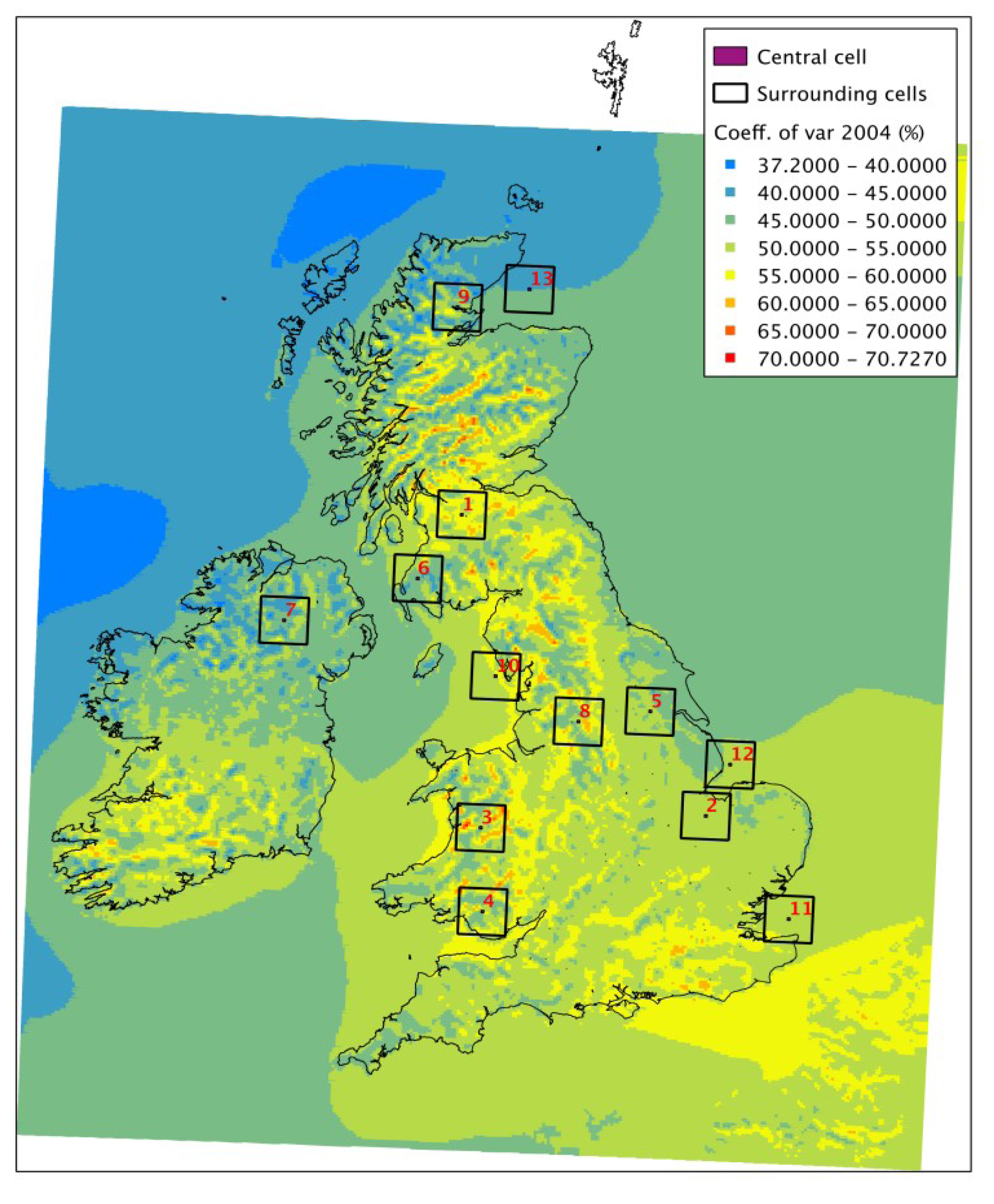
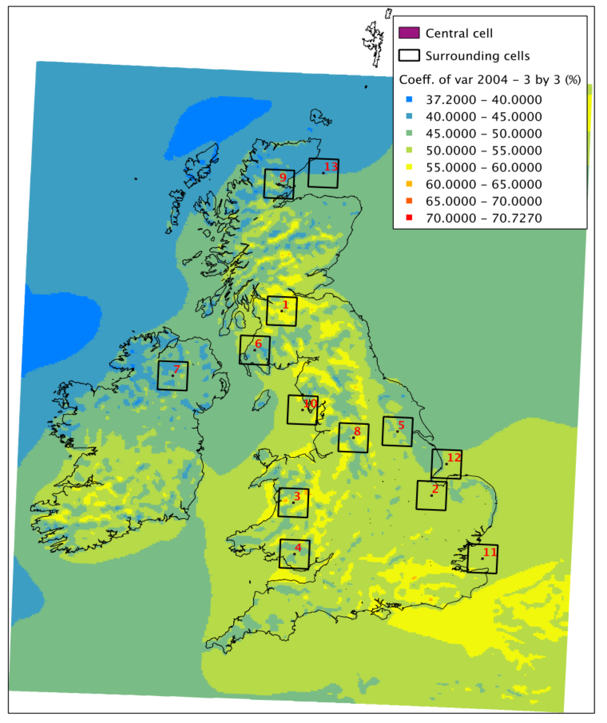
Throughout the work, results are presented generally for the whole WRF UK grid area, and in more detail for the locations highlighted in Figure 1, chosen for their proximity to wind developments and also to capture a broad range of physical characteristics related to location. The terrain and type of each location are classified in Table 1, and a ruggedness index, RIX, is calculated for each cell as:

(6)

where H_centre is the elevation of the centre cell, and H_i is the elevation of each of its 8 surrounding cells. Figure 1 also indicates the location of the met stations cited in [2].

Figure 1. Selected Weather Research and Forecasting (WRF) cells for detailed analysis.

Figure 1. Selected Weather Research and Forecasting (WRF) cells for detailed analysis.

Table 1. Description of sites chosen for detailed analysis.

Site	Name	General classification	Capacity in zone (MW)	Mean height (m)	Height range (m)	Ruggedness Index (RIX) (m)
1	Ayrshire	Inland	764	172	332	128
2	The Wash	Coastal	190	14	36	15
3	Central Wales	Inland	256	276	477	107
4	South Wales	Coastal	136	208	572	170
5	Yorkshire	Inland	140	25	120	9
6	Galloway	Coastal	347	126	461	146
7	Sperrins	Inland	141	151	314	69
8	Lancashire	Inland	146	227	453	205
9	Grampian	Coastal	305	178	732	168
10	Barrow	Offshore	608	0	0	0
11	Kent	Offshore	1205	0	0	0
12	Norfollk	Offshore	464	0	0	0
13	Aberdeen	Offshore	10	0	0	0

Table 1. Description of sites chosen for detailed analysis.

Site	Name	General classification	Capacity in zone (MW)	Mean height (m)	Height range (m)	Ruggedness Index (RIX) (m)
1	Ayrshire	Inland	764	172	332	128
2	The Wash	Coastal	190	14	36	15
3	Central Wales	Inland	256	276	477	107
4	South Wales	Coastal	136	208	572	170
5	Yorkshire	Inland	140	25	120	9
6	Galloway	Coastal	347	126	461	146
7	Sperrins	Inland	141	151	314	69
8	Lancashire	Inland	146	227	453	205
9	Grampian	Coastal	305	178	732	168
10	Barrow	Offshore	608	0	0	0
11	Kent	Offshore	1205	0	0	0
12	Norfollk	Offshore	464	0	0	0
13	Aberdeen	Offshore	10	0	0	0

3. Results

3.1. Interannual Variability

The map of interannual CVar is shown in Figure 2A for 10 m and Figure 2B for 80 m wind speeds. The interannual variability over this 11-year period is lower and more spatially consistent in most far offshore areas than it is onshore, with the exception of an area in the North Sea to the east of the northern UK. It has not been possible to establish if this area of difference is a model artefact or is indeed a true reflection of the variability here, possibly caused by storm track patterns or similar [11].

Figure 2. Interannual co-efficient of variation (%) for the annual mean 10 m (A) and 80 m (B) wind speed in a 10 year hindcast.

Figure 2. Interannual co-efficient of variation (%) for the annual mean 10 m (A) and 80 m (B) wind speed in a 10 year hindcast.

The onshore areas with the largest interannual variability are in regions of complex, and often coastal, terrain in Scotland, Wales and south-west Ireland. For the selected points in Figure 1, a box plot of the mean speeds for the 11 years is shown along with the coefficient of variation for each point in Figure 3.

The difference between 10 m and 80 m values is small, but the CVar at 80 m is slightly lower for most points. The patterns over the UK and Ireland region, as seen in Figure 2 are very similar.

Figure 3. Interannual statistics for selected points: (A) 10 m a.g.l; (B) 80m a.g.l.

Figure 3. Interannual statistics for selected points: (A) 10 m a.g.l; (B) 80m a.g.l.

3.2. Spatial Variability of the Long-Term Mean

It is interesting to capture the spatial variability in the long-term mean wind speeds found in sub-regions of varying size within the grid. Each WRF grid cell is 3 km by 3 km. Starting with a “window” of 3 cells by 3 cells (around 81 km²), increasing to 99 by 99, the long-term mean annual wind speeds have been used to derive the coefficient of variation for the centremost cell as in [12]. Referring to Equations (1) and (2), x_i represents the mean annual wind speeds of the n individual cells in the window; x is then the long term mean of the central cell, so that the variation over the region is calculated relative to the cell in question.

Figure 4 shows how the CVar of the long-term mean wind speeds within a window, in general, increases with increasing window size. This would be expected, as the larger windows capture more diversity in terms of terrain and conditions, leading to a wider variation in the long-term means within the window space. There are a number of areas having points with high coefficient of variation even over small window sizes, indicating that the mean annual wind speed can vary up to 30% over distances of less than 10 km. These areas typically have complex topography, so this result is expected. In contrast, there are some areas onshore in the UK and Ireland—flat regions far from the coast—which maintain relatively low values even over the largest window size, such that the variability in the long-term mean over an area of 120 km × 120 km remains under 10%. This would reflect the homogeneity in the terrain in these locations. In the offshore areas beyond a boundary approximately 100 km from shore, where little spatial variation would be expected, the variability within the largest window is under 5%. All window sizes highlight the transition from on- to offshore where significant changes will occur at the land-sea boundary. The range of the maximum coefficient of variation remains around 30% to 35% over all the windows.

Figure 4. Coefficient of variation in long-term mean wind speed from 11 year hindcast for varying spatial windows—(A) 3 by 3; (B) 15 by 15; (C) 35 by 35; (D) 59 by 59.

Figure 4. Coefficient of variation in long-term mean wind speed from 11 year hindcast for varying spatial windows—(A) 3 by 3; (B) 15 by 15; (C) 35 by 35; (D) 59 by 59.

Qualitatively, the spatial CVar of the long-term mean wind speed, particularly at smaller window sizes, looks related to the terrain complexity. Assuming a linear relationship, the linear correlation coefficient between CVar and the average ruggedness index, RIX, for the window has been calculated over all points for a series of increasing window sizes. As shown in Figure 5, for a 3 by 3 window, the correlation with the coefficient of variation is strong, confirming a linear relationship at this scale, and indicating that for areas of complex terrain (high RIX), the variability within the window is, naturally, higher. As the window size increases, the correlation between variability and RIX reduces considerably as the influence of terrain reduces in the overall calculation. The correlation then begins to increase slightly as the window size grows beyond 60 by 60 cells, or 180 km × 180 km. This might suggest that there is perhaps a reduction in some other influence after this point, possibly reflecting the scale of the weather systems affecting the country. The WRF model also makes assumptions about land-use for each grid cell, and hence a generalised roughness length, the effects of which may be contributing here.

Figure 5. Correlation between the ruggedness index (RIX) and coefficient of variation for differing window size.

Figure 5. Correlation between the ruggedness index (RIX) and coefficient of variation for differing window size.

Again, focussing on the spatial variation of the long-term mean, taking the cells highlighted in Figure 1 and increasing the window size shows a number of interesting features (Figure 6).

▪

The offshore points (10–13, shown in the upper panel) initially show a steady increase in variability with increasing window size; this rate of increase reduces at greater distances;

▪

The two very flat onshore locations (2 and 5) show similar trends to the offshore points and are plotted with the offshore points in the upper panel;

▪

The points located in more complex terrain (lower panel), however, show a lot of changes, both increases and decreases in the CVar, with increasing distance. This would be indicative that hills and valleys are causing peaks and troughs in the mean wind speeds of cells within the windows, but their effects are averaged out as the window size increases;

▪

Point 9 is a “rogue” point, compared to the others—it has a much larger variability from the beginning, and as the window size increases beyond 60 cells, it continues to trend upwards. This may reflect its location in both complex and coastal terrain;

▪

After a certain distance—depending on the location—the influence of terrain will be minimised and it is postulated that it is overtaken by the influence of mesoscale weather systems.

Figure 6. Change in coefficient of variation (CVar) with window size (A) offshore and flat onshore sites; (B) more complex onshore and coastal sites.

Figure 6. Change in coefficient of variation (CVar) with window size (A) offshore and flat onshore sites; (B) more complex onshore and coastal sites.

3.3. Effects of Spatial Aggregation

So far, the analysis has focused on the spatial variation of the long-term mean wind speed. In order to understand how the representation of hourly variability is affected by spatial aggregation of the model data—that is, averaging the time series over a wider area—a series of calculations have been run for each grid cell for a year. Firstly, for a given year, the hourly coefficient of variation for the cell has been calculated using the equations appropriate for the Weibull distribution (4 and 5). Then, for the same cell, a mean hourly wind speed has been derived using a “window” of surrounding cells over a given area, and the new hourly coefficient of variation has been calculated.

For the year 2004—chosen as an average year for the decade, see [11]—the original coefficient of variation for the UK is shown in Figure 7. The re-calculated CVar, based on a 3 by 3 window of cells (~9 km²) around the centre cell is shown in Figure 8, whilst Figure 9 shows a 9 by 9 window (~27 km²).

Figure 7. Coefficient of variation for 2004 (calculated from fitted Weibull parameters at each cell).

Figure 7. Coefficient of variation for 2004 (calculated from fitted Weibull parameters at each cell).

Figure 8. Coefficient of variation for 2004 (calculated from fitted Weibull parameters from the average of a 3 by 3 window around each cell).

Figure 8. Coefficient of variation for 2004 (calculated from fitted Weibull parameters from the average of a 3 by 3 window around each cell).

Figure 9. Coefficient of variation for 2004 (calculated from fitted Weibull parameters from the average of a 9 by 9 window around each cell).

Figure 9. Coefficient of variation for 2004 (calculated from fitted Weibull parameters from the average of a 9 by 9 window around each cell).

For a series of increasing windows, the change in the coefficient of variation indicates how the averaging process is smoothing out variations in the time series. The effect is more pronounced in areas that had points of high coefficient of variation in the first place. These points are limited in influence in the original map, with CVar decreasing rapidly with distance from the original cell, and thus are fairly quickly “averaged” out of the data. There is virtually no change in the coefficient in offshore areas, even for very large windows—again, expected, given that the spatial variability offshore is more consistent. There are some onshore areas, particularly in the flatter east and south east of England, where this is also the case. This would be a good indication that lower resolution models or single met station measurements would be good enough here to characterise wind generation over a relatively large area. It is also important to note here that at 3 km resolution, the WRF model is, therefore, itself an average and may be a lower average of the variability that would be manifest in higher resolution or point data in very complex terrain. In the areas of very high CVar—for example, in the Scottish Highlands—a higher-resolution model or a more dense installation of met masts might be appropriate.

Due to the computational time required, it is not reasonable to calculate the coefficient of variation for a large number of window-sizes for the entire grid. For the selected points, however, the CVar with increasing averaging window-size up to 75 by 75 (i.e., approximately 225 km × 225 km) is shown in Figure 10. For the offshore and smooth onshore points (upper panel), the CVar decreases with increasing window size, more slowly at first but then decreasing steadily after some point between 10 and 20 cells. For the more complex onshore points, there is an initial increase in CVar, before the value begins to decrease more steadily, again at a window size of around 10–20 cells. This represents a distance of around 30–60 km, likely the result of mesoscale weather influences overtaking that of terrain effects.

Figure 10. Coefficient of variation with averaging of cells for different points. (A) offshore and flat onshore sites; (B) more complex onshore and coastal sites.

Figure 10. Coefficient of variation with averaging of cells for different points. (A) offshore and flat onshore sites; (B) more complex onshore and coastal sites.

3.4. Discussion of Wind Variability Analysis

The results so far indicate that there are clearly areas within the UK where for the purposes of wind generation studies, single measurement points or low resolution models may suffice to capture the variability in output. Regions such as those far offshore, or with more homogeneous terrain, were identified in Section 3.1 as having typically lower interannual variability. It was shown in Section 3.2 that these offshore and homogeneous regions also exhibit less spatial variation in the long-term mean, even over large areas. It would be expected that patterns of wind generation across these areas will be similar.

Section 3.3 focused on analysis of the hour-on-hour variability in the wind speeds, and how spatial aggregation affects the temporal variability calculated for a region. The results reflect how models of lower resolution might represent temporal variability for different areas. It has been shown that for all of the regions, beyond a certain point where terrain influences are important, averaging the hourly wind speeds over wider areas steadily reduces the temporal coefficient of variation, i.e., the variation within the time series. It is identified in [16] that there is, however, a limit to this variability reduction as averaging regions begin to span very large areas. The author of [16] notes that some incidences of higher correlation seen between geographically disparate regions may relate to the scale of the weather conditions influencing the region.

If wind power generation were to be spread evenly throughout the averaged window (as was approximately the case in [5]), it could be assumed that the variability of the estimated power output would also decrease, at least up to a point. Hasche [17] finds that for 50 uniformly distributed wind farms within a region, this is indeed the case and for this number of farms, there is a relatively low sensitivity to how the capacity is arranged between the farms. A low resolution model would offer a reasonable approximation to derive an aggregate regional wind output in this case. However, wind capacity is not evenly distributed around the UK and where the generation is located in, for example, one corner of a low resolution grid cell, averages would potentially not reflect the true output of the system, especially in areas with highly variable wind speeds.

4. Impact on Power Analyses

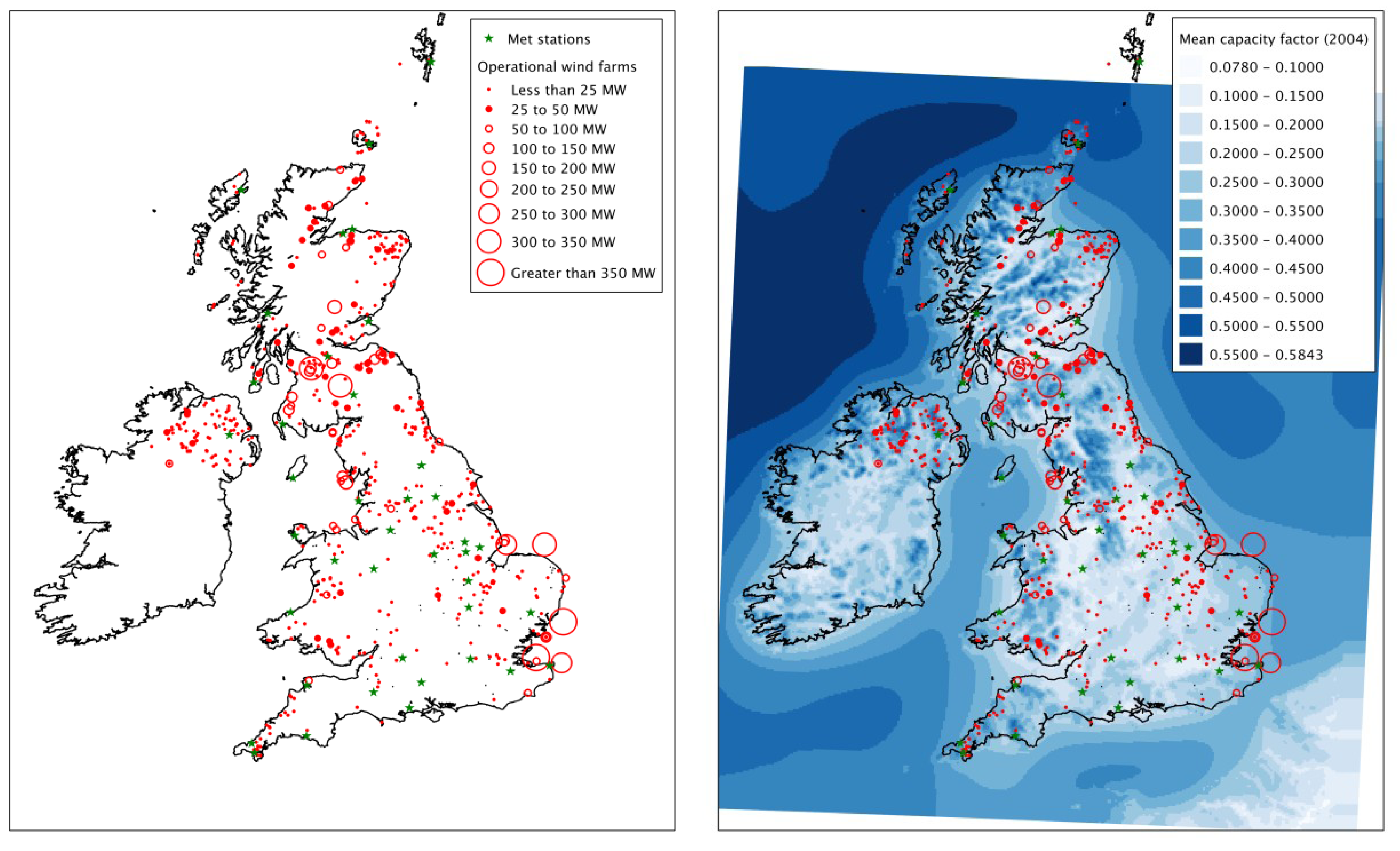
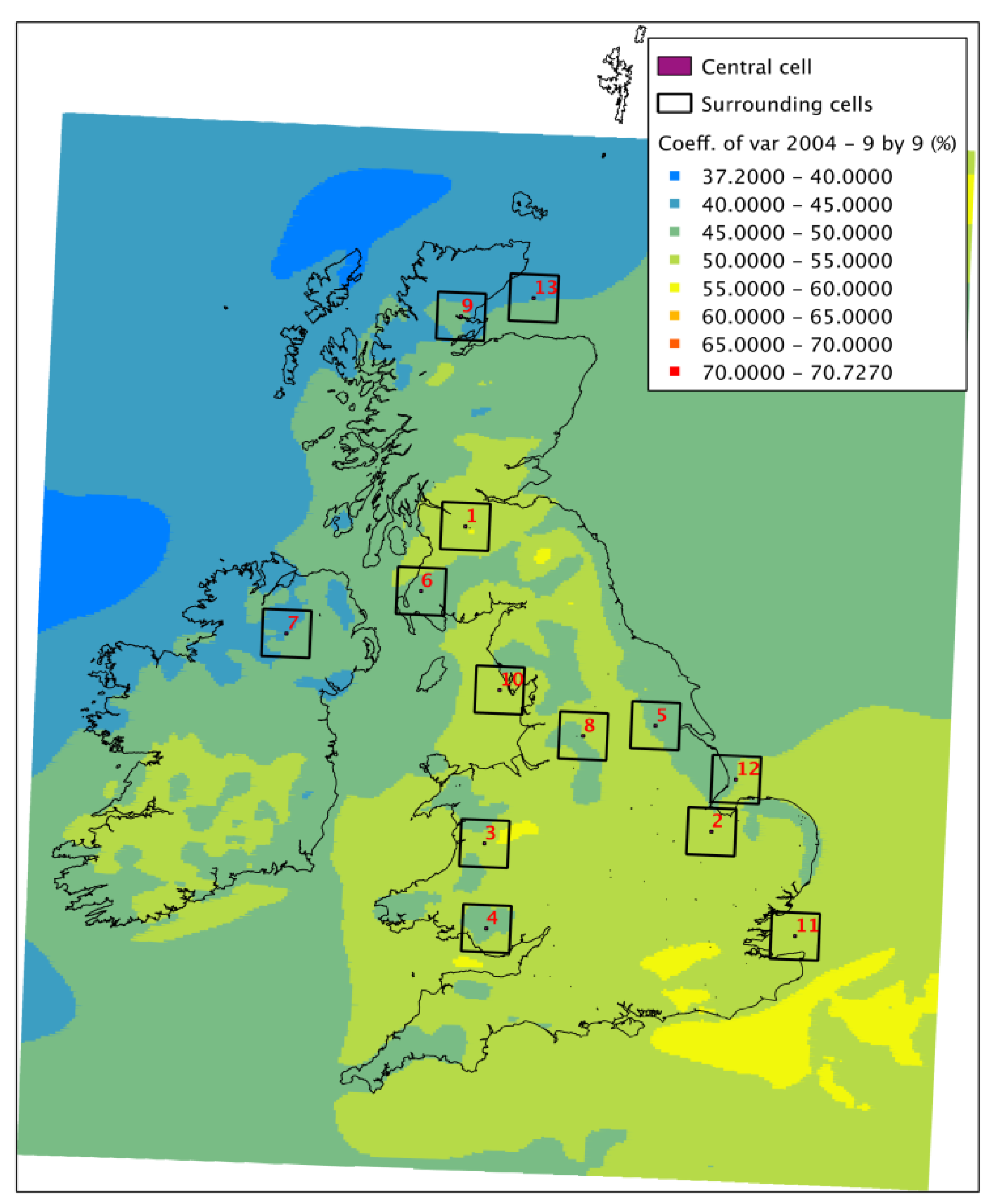
To demonstrate the case that the specific location of generation is a key factor in deriving aggregate power estimates, the statistics on the location, capacity and operational start-date for all the wind farms in the UK have been obtained from [15]. Figure 11 offers a visualisation of the operational wind generation capacity around the UK (as of October 2013). There is a concentration of relatively large-scale onshore generation to be found in Scotland, with developments in England, Wales and Northern Ireland being somewhat smaller. Offshore generation is largest along the east coast of England, with some smaller developments in the northwest of England. It is not necessarily the case that a met station network will match the locations of wind power capacity—this is highlighted in Figure 11, showing the met stations used in [2] (onshore, green stars). The areas with the highest density of onshore wind in central and southern Scotland have a low concentration of met stations, whilst there are a large number in the south and midlands of England, along with a lower density of wind capacity. This is likely to lead to some degree of bias in any aggregate UK-wide power where met station location is assumed to match capacity location. Figure 11 also shows the mean capacity factor for 2004 of a generic wind farm calculated for each cell in the WRF grid.

Figure 11. Met stations and wind capacity.

Figure 11. Met stations and wind capacity.

To demonstrate the impact on power production analysis of choosing different wind speed data types, for the points presented in Table 1, a window of 17 cells around the central point has been drawn (approximately 50 km × 50 km, similar to the resolution of recent reanalysis datasets such as MERRA [6]). The capacity of wind generation within the windows is given in Table 1. Three methods have been used to examine the power outputs for these regions:

▪

Pseudo-Met Station: The capacity factor of the central cell is taken as the capacity factor for the whole region;

▪

Lower resolution model: An 80m wind speed time series has been created as the mean wind speed of all the cells falling within the specified ~50 km × 50 km zone, and converted to capacity factor using the aggregate power curve;

▪

True”: The 80 m wind speed for the relevant WRF cell for each wind farm within the given radius is extracted and converted to power using the aggregate power curve scaled to the capacity of that farm. All the farms in the zone are then summed and the hourly regional capacity factor calculated as the aggregate power divided by the regional capacity;

▪

For 4 of the 50 km × 50 km areas (1, 5, 6 and 8), a met station falls within the zone, and for zone 2, one lies 10 km outside the boundary. Wind speeds for these met stations have been extracted for the time period of analysis, extrapolated from 10 m to 80 m turbine hub height (using a 1/7 power law) and the aggregate power curve applied to give a regional capacity factor.

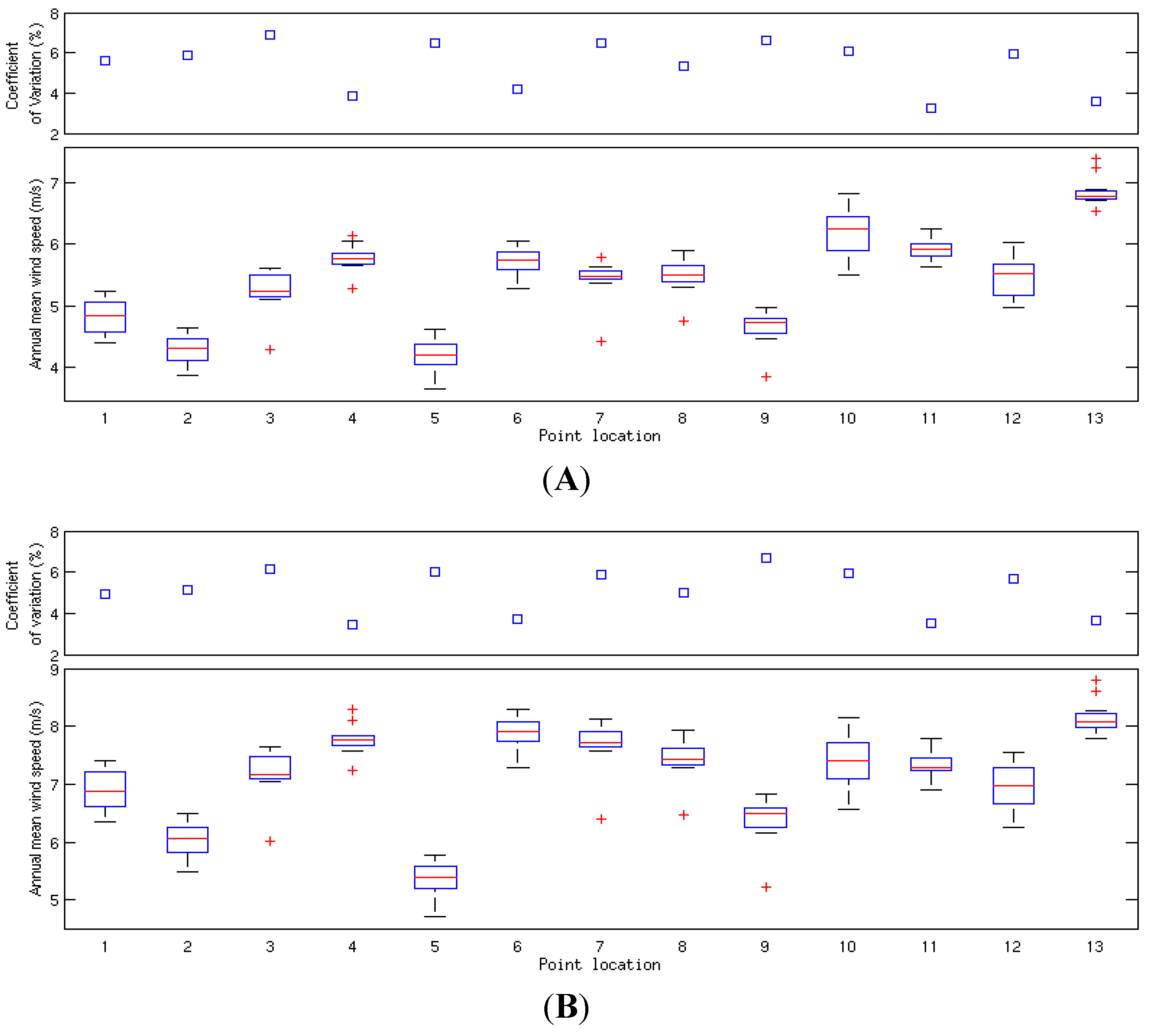
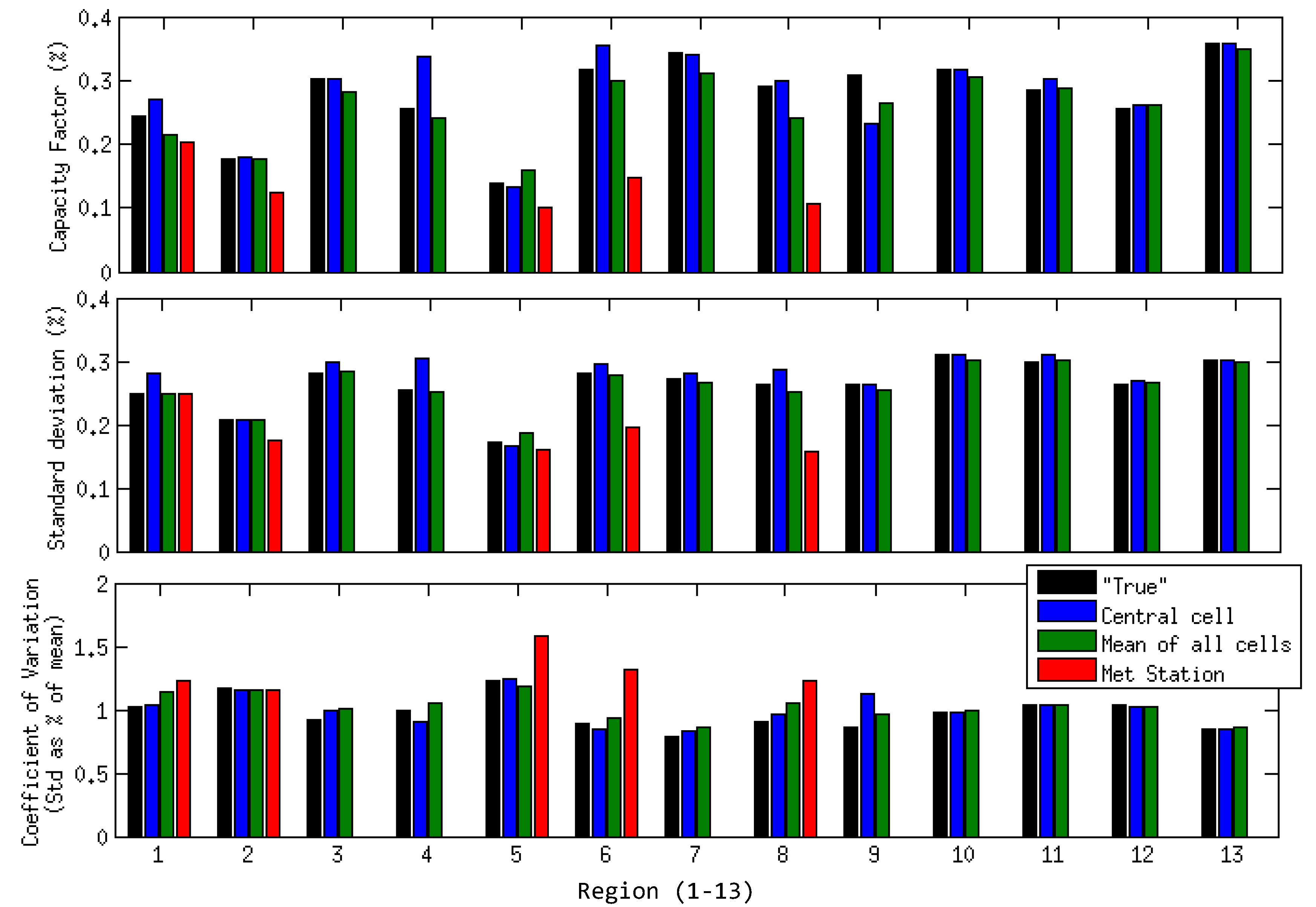
Figure 12 presents the mean 2004 capacity factors, standard deviations and coefficients of variation for each region as calculated using the methods outlined.

Figure 12. Mean capacity factors, standard deviations and coefficient of variation per region (1–13).

Figure 12. Mean capacity factors, standard deviations and coefficient of variation per region (1–13).

In 8 cases, including point 13 in which the single wind farm is actually located in the central cell, the central point gives a good approximation to the “true” annual capacity factor—within ± 1%. At a further three points, it is within ± 4%, and the final two points, 4 and 9, the most significant deviation of ± 8% from the central cell approximation is found. A mean calculated over all cells leads to an underestimate of the capacity factor in 9 out of the 13 zones. This could be explained by suggesting that in any given area, the wind farms would be expected to be located in the highest wind speed locations within that, so applying an overall mean—including the locations within the area with a lower mean wind speed, will give an underestimate of the mean power.

The maximum difference in the standard deviation calculations is 5% at point 4 using the central cell. A mean over all cells appears to provide a closer approximation to the standard deviation than the central cell method in many cases. Interestingly, however, the mean of all cells frequently overestimates the coefficient of variation. This is unexpected, given that regional averaging of wind speeds appeared to reduce the coefficient of variation, but is explained by the lower mean capacity factors. That is, although the standard deviation is similar, the mean power output is lower, and hence the ratio of the two quantities is found to be larger. For the offshore locations, the coefficient of variation is reasonably well approximated by both the central point and the regional mean. However, there are significantly different results at most of the other sites.

Where there is a met station available for the region, this appears to underestimate the mean capacity factor, by rather a large degree in most cases, except for zone 2. The station for zone 2 is around 10 km outside of the 50 km by 50 km area but was included as the wider region around here showed low wind speed variability in the previous section. At 4 out of 5 sites the standard deviation found using the met station is similar to the “true” value. Because of the lower estimates of mean capacity factor, the coefficient of variation is very much larger using the met station wind speeds, except for zone 2, where both the larger standard deviation and mean give rise to a consistent CVar. In addition, although the estimates based on met station data are measured rather than simulated data, the transposition from 10 to 80 m height will introduce uncertainty, as shown in [18]. It is conceivable that use of the log law rather than the simple power law used here might improve the match with the mesoscale model derived estimates, however this would be highly dependent on the assumed roughness lengths in each direction around the met station.

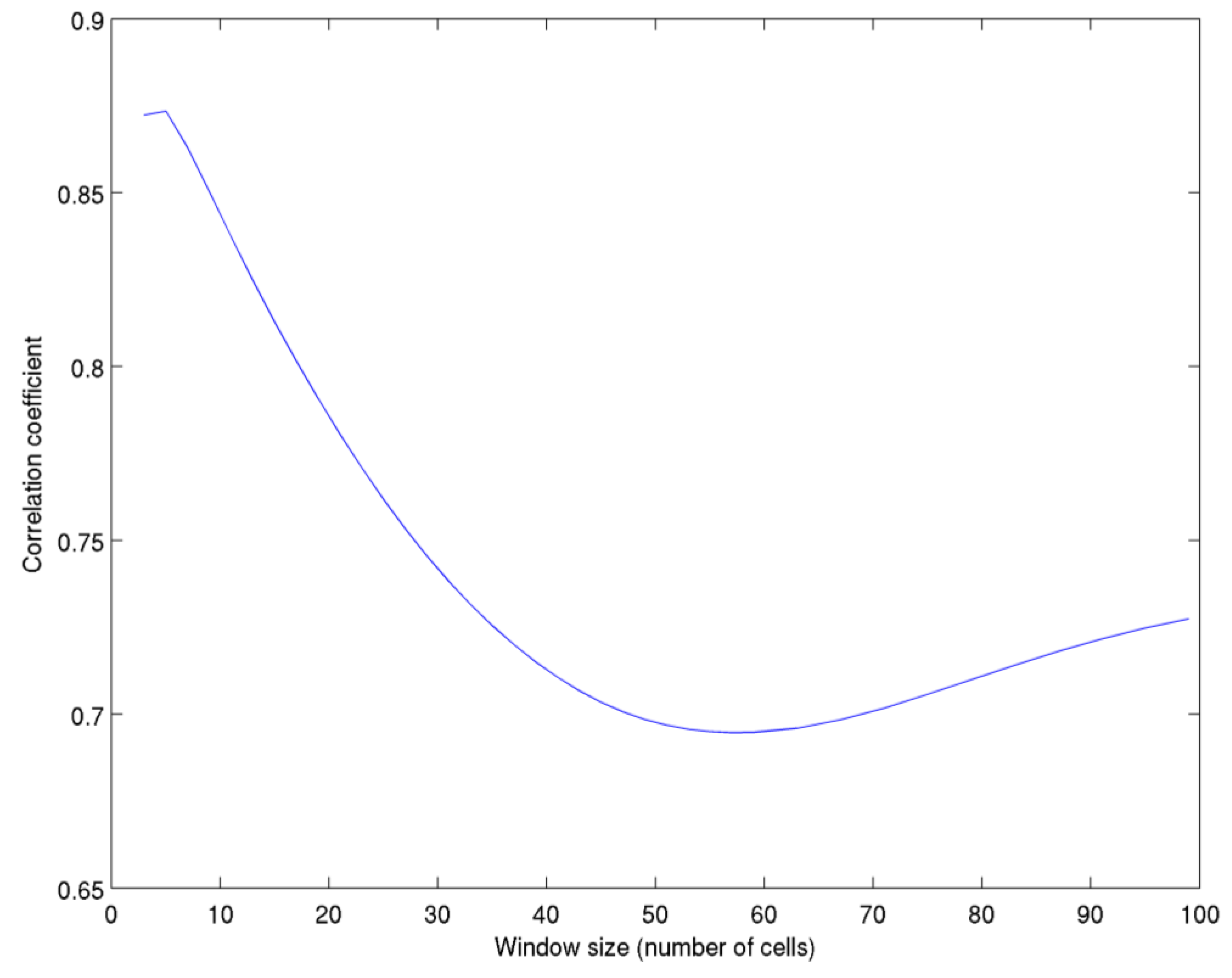
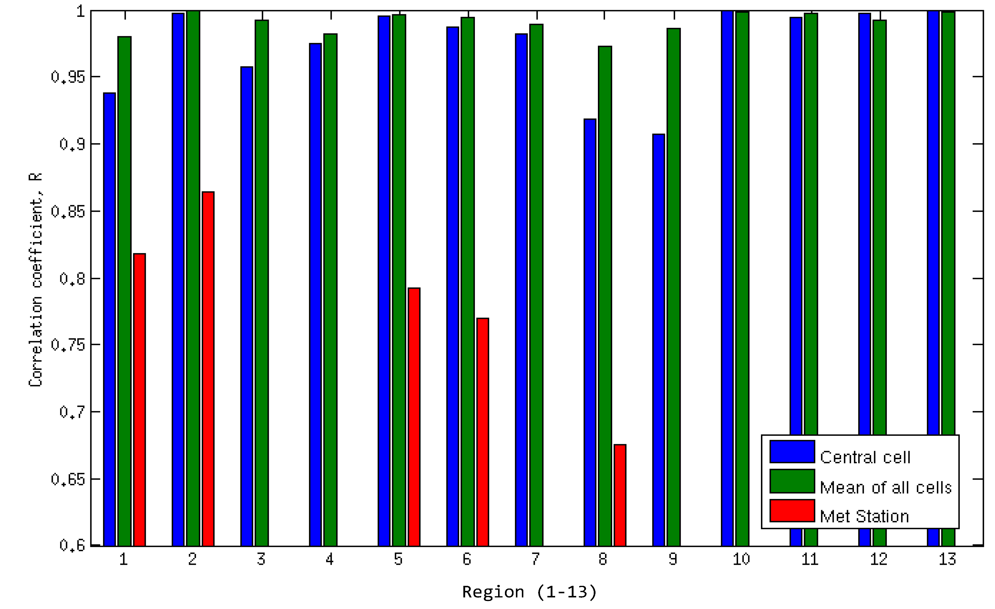
Figure 13 presents the linear correlation coefficient between the time series generated using the relevant WRF cells per wind farm (“true”) and the models using the central cell, the mean of all cells and, where available, a met station. Linear correlation is of more interest than a rank correlation here as the expected relationship between the variables is linear, rather than simply monotonic. The high values for both WRF-generated methods is not unexpected, and reflects the fact that these come from a single mesoscale model run, and the datasets in question are in close geographical proximity. For points 1, 8 and 9, the correlation coefficient using the mean and central cells compared to the actual wind power locations is a little lower than for other examples, suggesting high variability over these regions, or clustering of wind farms in non-average conditions. There are quite significant differences highlighted between the met station-derived series and the WRF series. For point 2, it is highest, and given the previous results, that is a reasonable expectation. For the other three points, however, the coefficient is decidedly lower.

Figure 13. Correlation coefficients of model time series compared to “True” capacity factors.

Figure 13. Correlation coefficients of model time series compared to “True” capacity factors.

The location of the central cell (or met station) and the location of the wind development are obviously crucial in the analysis. For areas of more complex terrain, if the central cell is in close proximity to the majority of the wind development, the power estimated from the central cell is reasonable and the correlation strong. 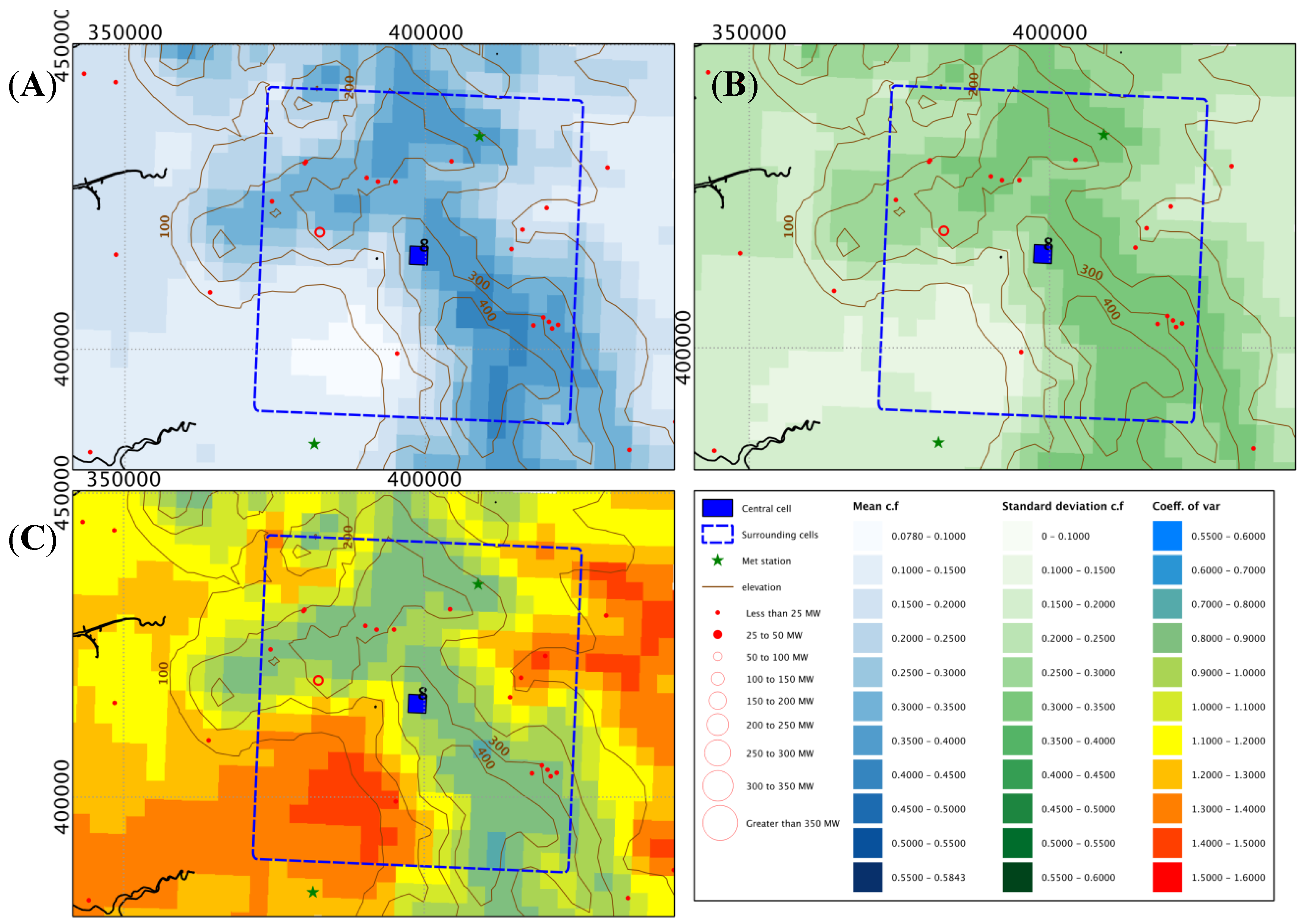If the wind developments are spread evenly throughout the 50 km × 50 km window, the mean of all cells gives a reasonable approximation, as was found in [5]. If, however, the wind developments are concentrated in one area, the two “guesses” are further away from the most accurate calculation. In particularly complex terrain, the correlations in time between the central cell and mean of all cells will be lower due to terrain factors influencing winds blowing in a particular direction that may only affect cells on a particular type of slope, for instance. 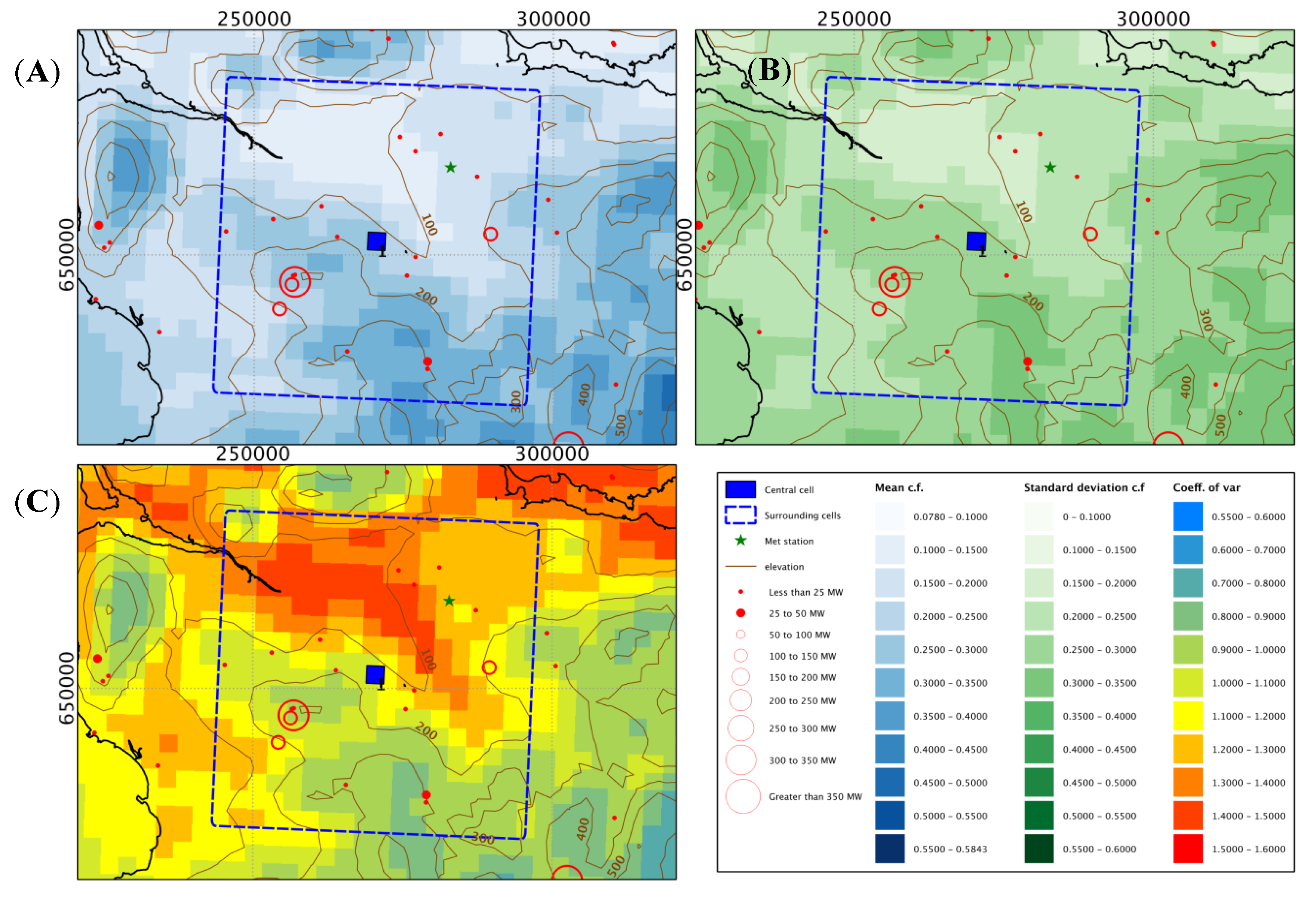For point 1, shown in Figure 14, the central cell is at a lower level than the largest wind developments and assuming westerly is the predominant direction, it is in the lee of the slope on which these large farms are situated, giving rise to the lower correlation in the time series of power estimates. The central cell for point 8 (Figure 15) is in an area of steep terrain, where the central cell is on top of a ridge, and most of the wind capacity is situated at a lower elevation, some on a differently oriented slope, again giving rise to a lower correlation in the power estimates.

5. Conclusions

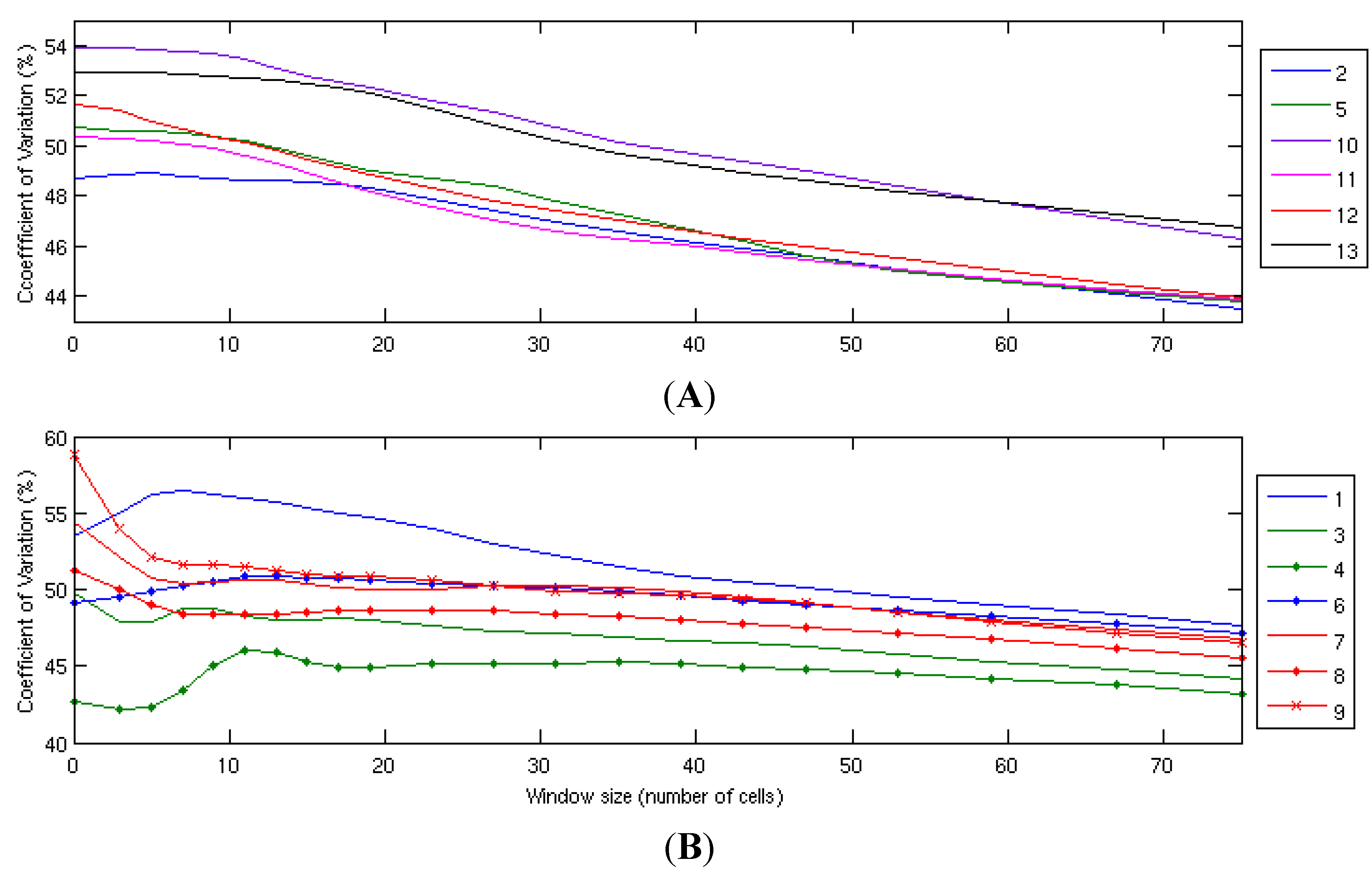
This work presents the characteristics of spatial and temporal variability in UK wind speeds based on decadal output from a high resolution mesoscale model, and the ramifications of using such data to generate an aggregate regional wind generation time series, compared to other methods using lower resolution models or met stations. The wind speed variability was found to be, as expected, dependent on the terrain and type of location under investigation, but it is clear that if the hourly speeds are averaged over wider areas, the variability does, beyond distances where topography is influential, decrease with increasing averaging area. This would be expected to have a similar effect on an aggregate regional power output, but the uneven distribution of wind power over the area is likely to cause biases in studies which assume an even distribution. It is, however, likely that in areas with lower variability, this biasing effect would be minimal.

Figure 14. Mean capacity (A), standard deviation (B) and CVar (C)—Point 1.

Figure 14. Mean capacity (A), standard deviation (B) and CVar (C)—Point 1.

Figure 15. Mean capacity (A), standard deviation (B) and CVar (C)—Point 8.

Figure 15. Mean capacity (A), standard deviation (B) and CVar (C)—Point 8.

Investigations of wind generation models for some localised areas of 50 km × 50 km showed that indeed, where the terrain is smooth and no coastal effects are present, either a single representative cell or an average provides a good estimate of the variability of the wind generation capacity factor for the region. Even a met station situated around 10 km from the edge of the window in the case of zone 2 gave a reasonably good approximation to the coefficient of variation of the wind power capacity factor, despite proportionately higher mean and standard deviations.

In contrast, those areas with uneven and complex terrain show a lot of variation across a 50 km by 50 km zone, and thus, where a met station is being used as a proxy, the location of said met station in relation to the installed generation is crucial to gain an accurate estimation of both the mean and variability of the wind production.