
Static and Moving Target Imaging Using Harmonic Radar
by
 ,
,
Kyle A. Gallagher
1, 
Ram M. Narayanan
2,*,
Gregory J. Mazzaro
3,
Anthony F. Martone
1 and
Kelly D. Sherbondy
1 1
U.S. Army Research Laboratory, Adelphi, MD 20783, USA
2
Department of Electrical Engineering, The Pennsylvania State University, University Park, PA 16802, USA
3
Department of Electrical & Computer Engineering, The Citadel, Charleston, SC 29409, USA
*
Author to whom correspondence should be addressed.
Electronics 2017, 6(2), 30; https://doi.org/10.3390/electronics6020030
Submission received: 31 December 2016
/
Revised: 17 February 2017
/
Accepted: 31 March 2017
/
Published: 4 April 2017
(This article belongs to the Special Issue Radio and Radar Signal Processing)
Abstract
:Nonlinear radar exploits the difference in frequency between radar waves that illuminate and are reflected from electromagnetically nonlinear targets. Harmonic radar is a special type of nonlinear radar that transmits one or multiple frequencies and listens for frequencies at or near their harmonics. Nonlinear radar differs from traditional linear radar by offering high clutter rejection and is particularly suited to the detection of devices containing metals and semiconductors. Examples include tags for tracking insects, tags worn by humans for avoiding collisions with vehicles, or for monitoring vital signs. Such tags contain a radio-frequency (RF) nonlinearity, often a Schottky diode, connected to a suitable antenna. Targets with inherent nonlinearities, such as metal contacts, semiconductors, transmission lines, antennas, filters, and ferroelectrics, also respond to nonlinear radar. In this paper, the successful exploitation of harmonic radar for moving target imaging and synthetic aperture imaging of targets, while suppressing clutter signals from linear targets, are presented. Our results demonstrate some unique advantages of harmonic radar over its traditional linear counterpart.
1. Introduction
One of the earliest observations of nonlinearities in electrical circuits was made by Michael Faraday in 1833 [1]. He observed that the resistance of particular resistors changed as a function of temperature. The modern day realization of this effect is the thermistor. A system is considered linear if it satisfies two properties, namely, homogeneity and additivity. A system is homogeneous if scaling the input to the system results in a scaled version of the output. A system is additive if, when multiple inputs are summed, the result is the sum of the outputs. Systems that do not meet both of these conditions are considered to be nonlinear systems. In a practical sense, all radio frequency (RF) and microwave systems exhibit some degree of nonlinearity; there is no such thing as a true linear system, only good linear approximations of nonlinear systems.
Nonlinearities in RF and microwave system can take many forms. Historically, nonlinearities are found in circuit elements such as diodes, transistors, amplifiers, mixers and others. A less common nonlinear mechanism is passive intermodulation (PIM) distortion, which is found in antennas, cable connectors, metal-to-metal junctions, etc. A recent development is the exploitation of nonlinearities in electronic circuits in order to detect and track nonlinear targets. This is typically done by tagging targets of interest with custom made nonlinear circuits.
Circuit elements exhibit nonlinear properties either by design or by consequence. By design, P-N junctions, such as diodes, are inherently nonlinear. The nonlinear effects of diodes are especially important in the field of RF for their use in mixers, which are used to up- and down-convert signals from one frequency to another. The operation of mixing two signals together to create a new frequency is a nonlinear operation. Upconverting signals to higher frequencies allows for higher bandwidths, thus information can be transmitted faster [2]. By consequence, many RF and microwave circuit elements exhibit unintended nonlinear properties. The best example of this phenomenon is the amplifier. Amplifiers are generally expected to operate linearly, and boost the input signal without creating extraneous frequencies at the output. In practice, building an ideal linear amplifier is not possible. As a result of an amplifier’s inherent nonlinear character, extra frequency content will be generated and possibly distort the desired signal. The unintended frequency content generated by the nonlinear properties of the amplifier can interfere with other radar and communication systems [3,4,5] as well as affect the sensitivity of the receiver. Much research has been done to linearize amplifiers [6,7,8,9,10].
Many nonlinear effects occur which are subtler and do not manifest themselves as often. Among these, the most prevalent is PIM, which is observed when high power signals interact with components that are weakly nonlinear. Weakly nonlinear components do not exhibit measurable nonlinear distortion under normal conditions. An early example of PIM in a RF system is the Luxembourg effect or cross-modulation, which was first observed in 1933 when a high-power radio transmitter caused interference to other radio stations by modifying the conductance of the ionosphere [11,12]. A more recent example of PIM causing unintended nonlinearities occurs in mobile phone towers, which communicate with multiple users simultaneously. PIM distortion in mobile phone towers is generated by the antennas and connectors [13,14,15,16,17]. Lesser known observations of nonlinearities come from electrothermal coupling. As components heat and cool, they begin to exhibit nonlinear properties, which are generally very weak [18].
Starting in the 1970s, research began focusing on detecting, measuring, and exploiting nonlinear circuit elements at standoff distances. Most naturally occurring objects do not exhibit significant nonlinear characteristics [19,20]. This permits detection of small nonlinear objects in the presence of larger linear clutter. Theoretical and experimental data have shown that different nonlinear junctions can be discriminated against at standoff distances [21,22,23,24,25,26,27,28,29,30]. These systems traditionally operate at a single frequency and detect nonlinear devices connected to an antenna.
A harmonic radar (a specialized form of nonlinear radar) transmits a frequency and processes returns at a harmonic frequency , where . Usually, the second harmonic, i.e., , is used since it generally provides the strongest response from these types of targets. This radar approach effectively separates the harmonic target response from the clutter band, thereby making harmonic radar attractive for several applications. The automobile industry has been investigating harmonic tags as early as the 1970s for avoiding collisions with other automobiles and humans carrying nonlinear tags at X-/Ku-Bands [31,32,33]. Such a system has also been used by biologists and entomologists interested in tracking insects at 917/1834 MHz [34,35] and at 5.8/11.6 GHz [36,37,38].
Since most systems traditionally used a single frequency waveform and a single transmit and receive antenna, only detection of nonlinear targets was performed. No ranging, tracking, imaging or identification of nonlinear targets was possible. For two-dimensional localization of nonlinear targets, a wide bandwidth and a large aperture are needed to achieve good down range and cross range resolutions, respectively.
To address the shortcomings mentioned above, we have constructed a wideband harmonic radar operating transmitting over the 800–1000 MHz range and receiving over the fundamental frequency range as well as the second harmonic (1600–2000 MHz) frequency range [39]. In this paper, we present the basic principles of harmonic radar, and provide experimental evidence of its ability to suppress linear clutter, perform detection and indication of slow moving nonlinear targets, and perform high resolution synthetic aperture imaging. While our work on moving target and synthetic aperture radar imaging has been published in conference proceedings, this paper combines the two imaging modalities and presents a unified treatment of the two topics.
2. Harmonic Radar
2.1. Harmonic Radar Range Equation
A nonlinear scatterer can be characterized by a scattering radar cross section (RCS) that depends upon (and generally increases with) the incident power density , as opposed to a linear scatterer for which the RCS may be assumed constant except at very high power levels. The nonlinear RCS, in m2, is defined as that area intercepting the amount of power at frequency which, when scattered isotropically at frequency , produces an echo equal to that observed from the scatterer [40]. For nonlinear scattering to occur, ; however, for harmonic scattering, is a multiple of . Over the past few decades, several researchers have characterized the nonlinear scattering properties of a variety of targets, both analytically and experimentally, and have also derived different formulations for the nonlinear radar range equation [41,42,43,44,45,46,47,48,49].
The radar range equation for a harmonic radar (, where is an integer) has been derived and it shows that, whereas the received signal is inversely proportional to the fourth power of the range for a conventional radar (i.e., dependence), the range law becomes increasingly unfavorable for successive higher harmonics, showing a dependence of [50]. For a practical harmonic radar, the second or third harmonics are therefore generally preferred, yielding inverse sixth and inverse eighth power range laws, respectively. Even so, the higher rate of power reduction with range restricts the use of harmonic radar to close range applications (less than about 20 m), although they have the advantage of higher visibility when illuminated at higher power densities.
Consider the block diagram of a radar signal path shown in Figure 1.
In Figure 1, point A represents the transmitted waveform, point B represents the waveform impinging on the nonlinear target after traveling a distance , point C represents the response from the nonlinear target, and point D represents the signal returned to the radar. The radar range equation can be derived in the standard manner.
We model the input–output relationship for the nonlinear device as a power series, as
where is the input power incident on the target, is the isotropically radiated output power by the target, and is a scaling coefficient for the nth harmonic of the nonlinear device. The coefficient has units of W1−n. The term represents the linear response, and the scaling coefficients generally drop off as increases, i.e., .
The radar range equation for the nth harmonic term has been derived as [51]
where is the fundamental transmitted frequency, is the received frequency at the nth harmonic, is the transmitted power, is the gain of the transmit antenna at frequency , is the gain of the receive antenna at frequency , is the wavelength corresponding to the nth harmonic at frequency , is the range to the target, and is the radar cross section of the target at the nth harmonic.
The radar cross section, , is given by [51]
where is the effective aperture area of the target at the fundamental transmit frequency and is the target aperture’s reradiation gain at the nth harmonic frequency .
2.2. Unambiguous Range and Range Resolution
In a wideband harmonic radar system, the transmit frequency is stepped over a bandwidth centered around a frequency in steps of . Consequently, the nth harmonic received at the radar, , has a bandwidth of centered around , due to the linear multiplication of the fundamental frequency band. For a harmonic radar operating at the nth harmonic, the maximum unambiguous range to the target, , and the down range resolution,, are given by, respectively [52]
and
where is the speed of light.
2.3. Description of Harmonic Radar
The block diagram of our harmonic radar system is shown in Figure 2. The system transmits a stepped frequency waveform over the 800–1000 MHz range and processes returns at the fundamental and the second harmonic 1.6–2 GHz frequency ranges.
The signal is generated by a National Instruments (NI) 5651 synthesizer card. Next, a coupler is used to tap off a small amount of the signal that is used as the reference. The signal is then filtered by two diplexers, each consisting of a high pass filter and a low pass filter allowing the separation of the fundamental frequency from the harmonics. The cutoff frequencies of the high and low pass filters are both set to 1.3 GHz. The cutoff of 1.3 GHz was chosen to lie between the highest fundamental frequency and the lowest second harmonic frequency. The highest fundamental () frequency is 1 GHz and the lowest second harmonic () frequency is 1.6 GHz. A power amplifier (PA) is used to amplify the signal to 10 W (+40 dBm). After amplification, additional harmonics are generated, so additional diplexers are utilized for suppression. Since the power at this point is 10 W, high-power cavity diplexers are used. Each diplexer provides >80 dB of rejection in the unwanted frequency range while only attenuating the desired signal by less than 0.5 dB. The receiver is very sensitive to any harmonic signals, including harmonics generated by the transmitter. For this reason, two diplexers are used to further reduce the harmonics. An isolator is used between the diplexers to isolate the power amplifier from reverse traveling waves. Possible sources of reverse traveling wave are signals entering the transmit antenna and mismatches between the diplexer and antenna.
In the receiver, a diplexer is used after the antenna to separate the fundamental and the second harmonic. The fundamental is sent directly into a LeCroy oscilloscope for digitization. Following the diplexer, the second harmonic is amplified in a low noise amplifier (LNA), filtered through four additional diplexers, amplified in another LNA, followed by a medium power amplifier (MPA). A MPA is used for the final amplification stage to reduce distortions. A 3-dB attenuator is added between the MPA and the LNA to improve the impedance match between them and to reduce reflections. A high-speed LeCroy oscilloscope is used to digitize the reference signal from the coupler, the second harmonic from the receiver, and the fundamental response. The oscilloscope is set to sample the signals at 10 GS/s.
Specifications of the harmonic radar system are presented in Table 1.
3. Imaging of Moving Targets
Military systems face a daunting task when confronted with a complex scene containing multiple moving targets as well as stationary and moving clutter [53]. They often attempt to separate moving targets from stationary objects based on (i) measurements of the range to target; and (ii) measurements of the Doppler frequency induced by target motion. Hence, target declarations are often made based on analysis of data transformed into the range-Doppler plane. Unfortunately, range-Doppler artifacts created by moving clutter objects (such as swaying trees) can often mask slowly-moving targets of interest [54,55]. In addition, the presence of a large number of moving targets may overload downstream processing of moving target indication (MTI) detections. If, however, the targets of interest produce nonlinear responses to a radar probe signal, it should be possible to further separate them from both background clutter and linear targets that are not of interest.
Until recently, the exploitation of non-linear phenomena has been restricted primarily to the detection of stationary targets [21,41,56]. If such non-linear processing techniques could be incorporated into an MTI processing framework, a substantial enhancement in MTI system detection capability could be realized. MTI data can be processed many ways. If a target is moving between multiple range bins as data are collected, change detection can be implemented to find the moving target [57]. If the target is moving slowly with respect to the data collection rate, the target remains fixed within a single range bin and Doppler processing is needed. If the data are phase-coherent, then a coherent processing scheme can be performed to create a range-Doppler plot to track the slow moving target.
Prior work on the use of harmonic radar to detect and characterize moving targets has primarily focused on insect tracking [58,59] and respiration monitoring [60]. In both these applications, appropriate RF tags are attached to the target’s body and the harmonically scattered signal is used for tracking or Doppler estimation. This suppresses the large scattering signals from large clutter objects and interfaces and permits the extraction of the Doppler response.
3.1. Moving Target Imaging Approach
In this development, a range-Doppler plot is created for the fundamental frequency () response as well as for the harmonic response (). Data were collected as a nonlinear target was moved to different ranges. At each target position, a full frequency sweep was performed. The frequency data collected at each target position spans the columns of a complexes data matrix. Each subsequent data acquisition fills the next row, which is called the slow time axis. An Inverse Fast Fourier Transform (IFFT) operation is performed across the rows to transform the frequency domain data into the fast time domain, which can then be transformed into the distance (or range) domain, as shown in Figure 3.
A Fast Fourier Transform (FFT) is then applied to each column transforming the slow time domain data into the Doppler frequency domain, as shown in Figure 4. In order to convert the Doppler frequency domain into the speed domain, scaling by the appropriate wavelength is needed.
From Fourier analysis, the maximum unambiguous Doppler frequency shift is based on the time pulse repetition interval (PRI). The PRI, , is defined as the time it takes to collect data from all frequency samples () to create one range profile. The maximum Doppler frequency, , is given by [61]
Dividing both sides by the number of complete data collections taken, , yields the Doppler frequency step size, , given by [61]
where the product represents the total amount of time it takes to collect data for one range-Doppler plot. This is called the coherent processing interval (CPI). Multiplying Equations (6) and (7) by the average wavelength yields the maximum unambiguous target speed, , and the step size or speed resolution, , for the speed axis, respectively, given by [61]
and
Applying these equations to the linear and non-linear responses results in an n-fold reduction in the unambiguous target speed for the n-th harmonic and an n-fold reduction in speed step size.
3.2. Moving Target Imaging Setup
MTI data were taken in an anechoic chamber with the nonlinear target placed 4.6 m (15 feet) from the radar, as shown in the setup in Figure 5. To simulate a moving target, the nonlinear target was moved in 2.5-cm (1-inch) increments away from the radar. A commercial RF mixer, manufactured by Mini-Circuits, was used as the nonlinear target. The antenna was connected to the RF port (as is the usual case in a receiver front end), and the local oscillator (LO) and intermediate frequency (IF) ports were terminated in 50 ohms. The mixer was not driven into its nonlinear region since there was no LO power injected. The no LO injection case (our case) is more challenging because the nonlinear response of the mixer diodes is lower than if the diodes were biased due to the injection of LO power [62].
An in-house built dual dipole antenna was used to get energy in and out of the mixer. Each time the target was moved, complex measurements at each of the 81 frequencies were taken for the linear and the nonlinear response. The second harmonic () range resolution was about 6 cm (15 inches), so moving the target 2.5 cm (1 inch) at a time kept it well within one range cell. Photographs from the test setup are shown in Figure 6.
3.3. Data Acquisition and Analysis
Data were taken over the 81 fundamental and 81 harmonic frequencies for each of the target locations. The raw data were zero padded in both the slow time and frequency domain. This was done to interpolate the range-Doppler plot. Figure 7 shows the MTI results. In order calculate the Doppler speed axis, a data collection rate of 48 Hz was chosen.
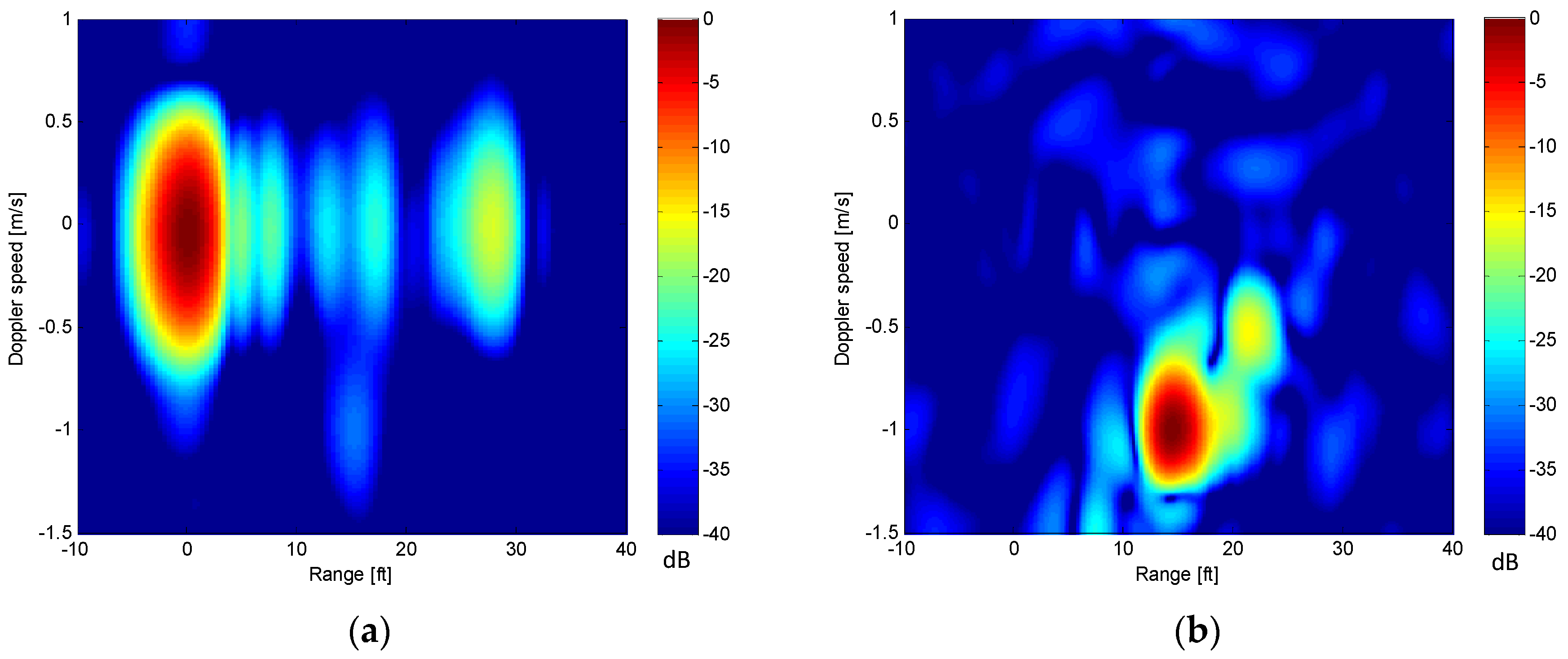
The image in Figure 7a shows the linear response of the mixer moving at the fundamental frequency, while the image in Figure 7b shows the nonlinear response of the mixer moving at the harmonic frequency. Figure 7 exhibits side lobes in both the range and Doppler domains. Therefore, a Hamming window is applied in both the frequency and the slow time domains to reduce the ringing caused by the sidelobes. The result is shown in Figure 8 for both the linear and nonlinear cases.
The effect of windowing is that the side lobes are reduced, albeit at the cost of widening the peaks. The linear () MTI plot shown in Figure 8a shows a strong response at zero range and zero Doppler, which can be ascribed to transmit–receive antenna coupling. Although the data were taken in an anechoic chamber, there is a response from the back wall at about 7.6 m (25 feet). Since the wall is stationary, the resulting response is located at zero Doppler. There are also other linear responses from the environment between the antennas and the back wall. The target can be seen between 4.6 and 6.1 m (15–20 feet) and −1 m/s. The linear response from the target is small and would otherwise be lost in the antenna coupling and clutter, but because it is moving, MTI processing is able to distinguish it from stationary targets.
For the second harmonic response, shown in Figure 8b, there is no antenna coupling at zero range and zero Doppler. In addition, the target response stands out as the largest object in the scene, and linear clutter is virtually eliminated. There is a second response from a target at a further distance and slower Doppler speed. This is likely due to multipath, as explained in [63].
Figure 9 clearly delineates different phenomenological mechanisms that more clearly expound upon the conclusions drawn above.
We did not perform any Doppler measurements outside the anechoic chamber. In realistic outdoor scenarios, radio frequency interference (RFI) can cause degraded performance since the level of these signals at the desired harmonic bands may overwhelm the low level harmonically scattered signals being processed by the radar. In addition, multipath may cause the formation of ghost targets in the image.
4. Synthetic Aperture Radar (SAR) Imaging
Wideband synthetic aperture radar (SAR) systems are known to produce high resolution images of target scenes. High resolution in the range direction is obtained using a wideband signal while high resolution in the azimuth direction is achieved by coherently processing the Doppler modulated returns as the antenna is scanned over a large synthesized aperture [64]. In this section, we show that a harmonic SAR can be used to form high resolution images of nonlinear targets and also be used to suppress linear clutter plaguing traditional linear SAR systems. Two different SAR data collection techniques have been implemented to create SAR images: a moving aperture, and a fixed aperture.
4.1. SAR Image Processing Approach
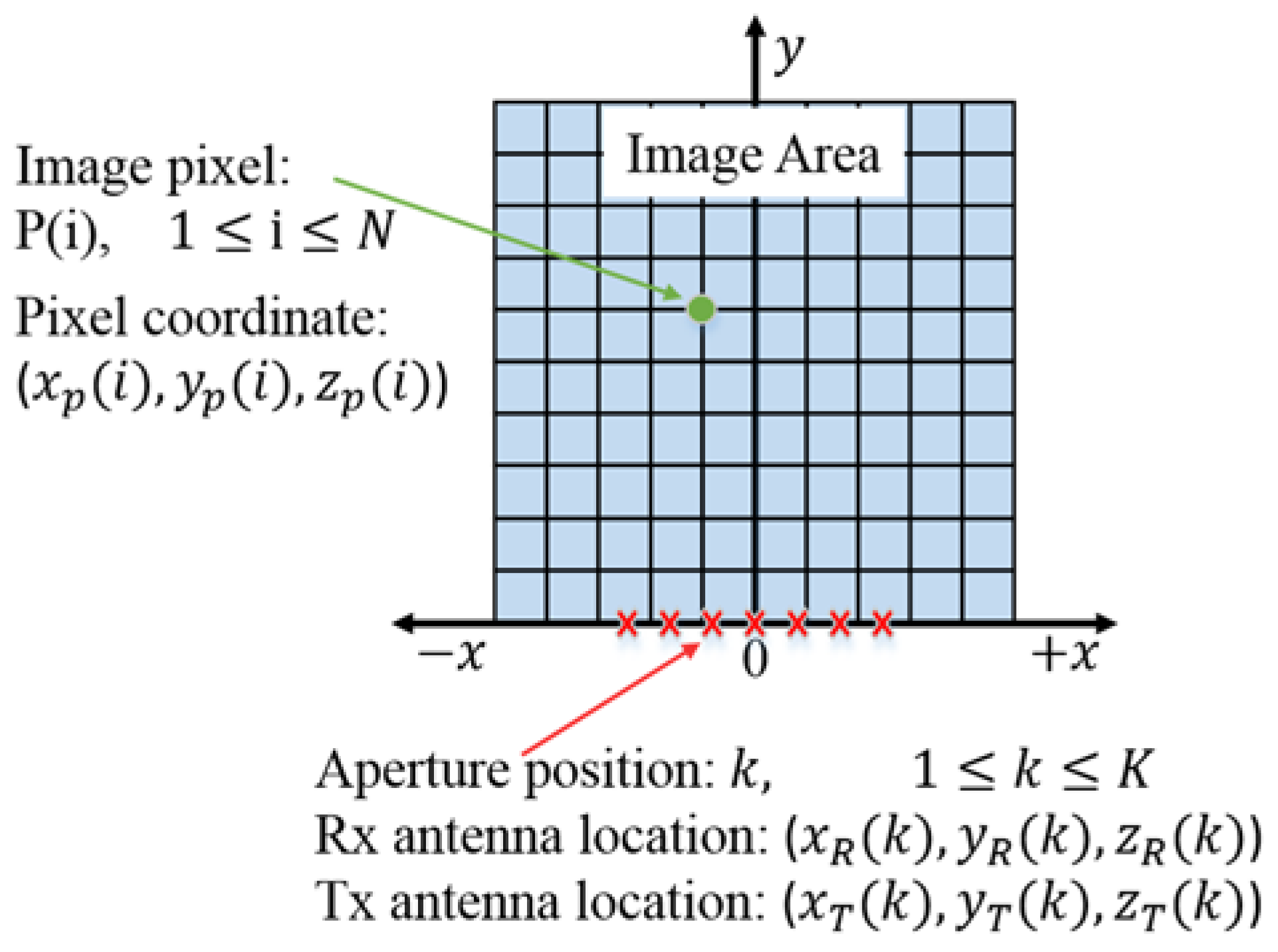
SAR images can be created using data collected in many different configurations. For airborne applications, SAR systems can fly in a straight line to image a large area or they can fly in a circular path to image a desired target [65]. Ground vehicle based SAR systems can be configured in a forward looking orientation [66,67,68] or a side looking configuration [69,70]. Regardless of the configuration and orientation, the basic imaging algorithms remain the same. The SAR data collected here use a back-projection algorithm to form the SAR images [66]. To perform the back-projection algorithm, a coordinate system, image area, and antenna positions need to be defined. The imaging area consists of pixels with coordinates and amplitudes , where . Data are collected over an aperture consisting of positions. The coordinates of the transmit and receive antennas need to be known at each of the positions. The location of the receive and the transmit antennas at each aperture position are denoted as and , respectively, where . An illustration of the back-projection algorithm is presented in Figure 10.
The coordinate system, images area and antenna position define the geometry of the scene. In addition to the geometric configuration, the range profiles at each aperture position are needed to create the image. The range profile at each aperture position is defined as , where is the delay and is the index of the aperture position.
The amplitude of each pixel in the image, , is calculated using
where , is the time delay from the transmit antenna at aperture location to the pixel at location plus the time delay from the pixel to the receive antenna, also at location . The delay from the transmit antenna to each pixel location is calculated using
where is the delay from the transmit antenna to the pixel and is the speed of light. Similarly, the delay from the image pixel to the receive antenna is calculated using
where is the delay from the transmit antenna to the pixel. The two-way delay, , is then given by
Now that the mathematics for SAR imaging have been established, SAR images can be created.
4.2. Moving Aperture SAR Imaging
4.2.1. Experimental Setup
The first set of SAR images was obtained from a moving aperture. Data were collected in an anechoic chamber to reduce environmental effects and multipath. A diagram illustrating the setup is shown in Figure 11.
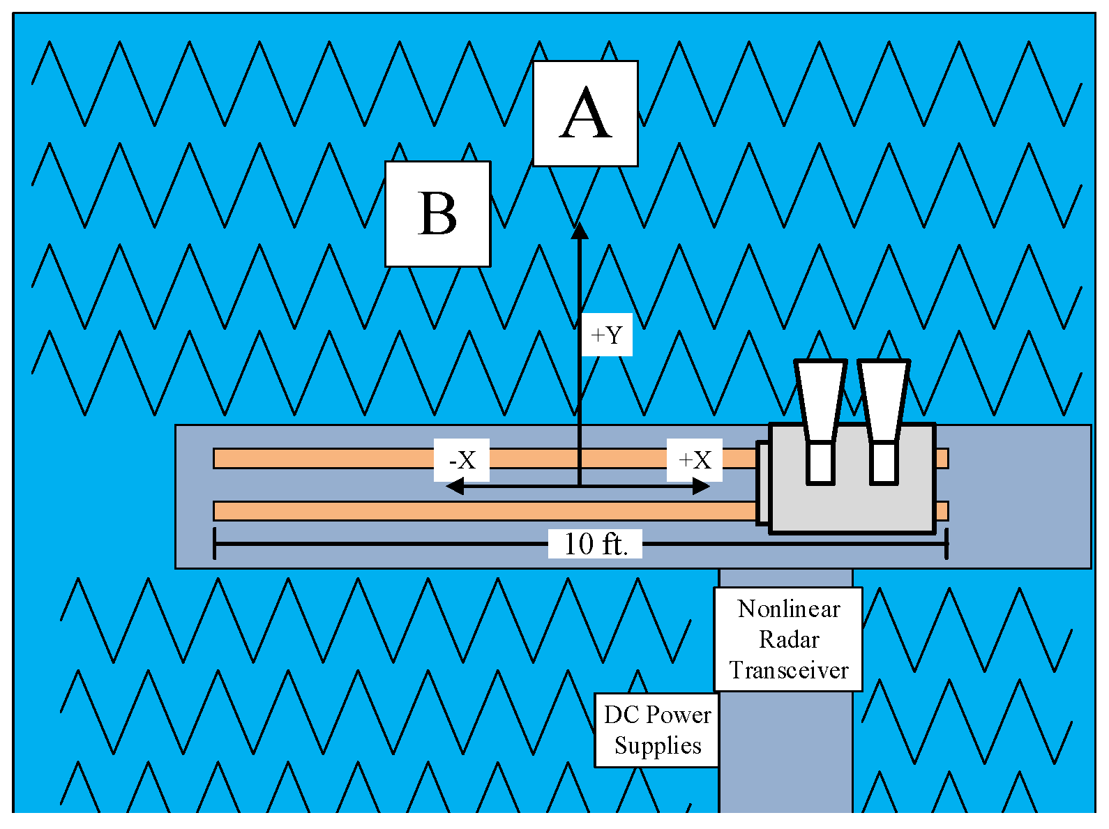
The antennas were manually moved along a 3-m (10-foot) aperture with a 5-cm (2-inch) step size. This yields aperture positions for the synthetic aperture. The target(s) remained stationary while the antennas were moved along the aperture, as shown in the coordinate system in Figure 11. The aperture was centered at and spanned from to . The radiating apertures of the antennas were located at . Targets were placed in one of two positions, A or B. The coordinates of points A and B are presented in Table 2.
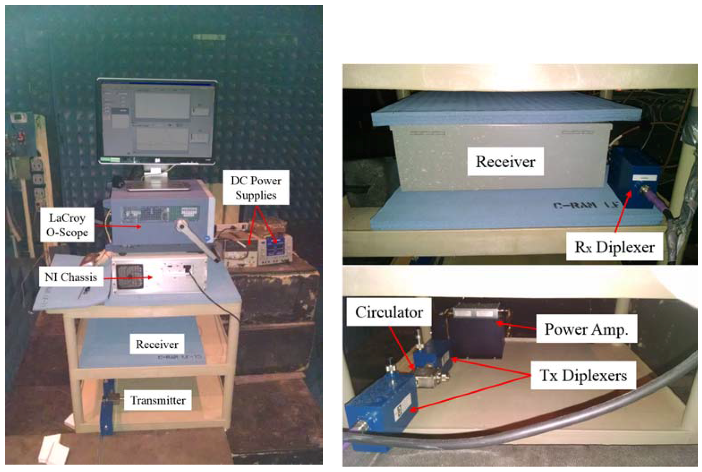
Photographs of the system hardware are shown in Figure 12.
As seen in Figure 12, the transmitter and receiver hardware were physically located close to each other. For this reason, the receiver was placed in a metal box and surrounded with absorbing foam to suppress leakage from the high power transmitter into the receiver.
To move the antennas along the aperture, the transmit and receive antennas were attached to a plastic cart on wheels. Two lines of duct tape were placed along the track to keep the antennas in proper alignment and to monitor the antenna position while in motion. Photographs of the cart, duct tape track, and antennas are shown in Figure 13.
4.2.2. Description of Targets
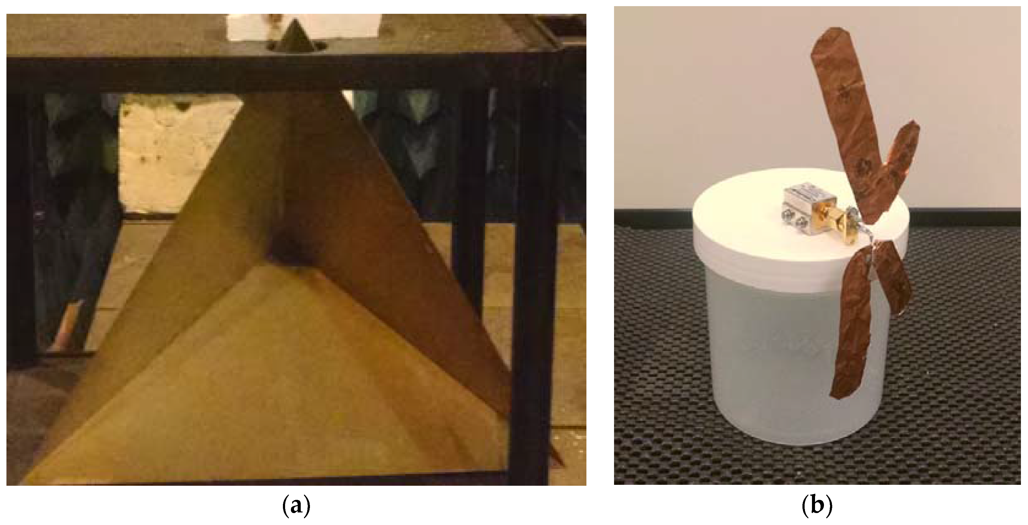
For the data collection, two targets were used, one linear and one nonlinear. The linear target was a trihedral corner reflector whose longest dimension was 50.8 cm (20 inch). The nonlinear target used was a commercial mixer with a custom antenna attached to the LO port. The antenna used was an in-house built dual band dipole antenna. The low frequency band of the antenna was tuned to 900 MHz and the high frequency band was tuned to 1800 MHz. These frequencies correspond to the center of the linear and the harmonic bands, respectively. Photographs of the targets are shown in Figure 14.
4.2.3. SAR Imaging Results
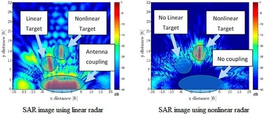
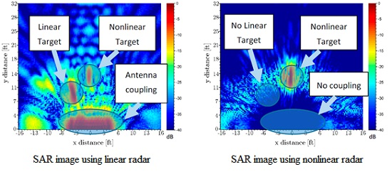
SAR images were generated using the step frequency data and the back-projection algorithm [66]. More details on harmonic SAR processing can be found in [71]. Linear and nonlinear SAR data were collected on both targets present in the scene using both the linear and the nonlinear radar. The mixer placed at position A and the corner reflector placed at position B (See Table 2 for location coordinates). The linear and harmonic SAR images are presented in Figure 15.
The linear response shows the corner reflector and mixer at the correct locations, while the nonlinear radar only shows the mixer and suppresses the corner reflector. Although the corner reflector was present in the scene while the nonlinear data were collected, it does not appear in the nonlinear SAR image in Figure 15b. This clearly demonstrates the advantage of nonlinear radar in detecting only nonlinear targets. The antenna coupling also shows a strong response in the linear SAR image, and it stays in the same range bin regardless of aperture position; thus, it is observed along the entire aperture, to .
Figure 16 clearly delineates different phenomenological mechanisms that more clearly expound upon the conclusions drawn above.
4.3. SAR Imaging with Fixed 16-Channel Receiver
4.3.1. Experimental Setup
In this section, we describe a fixed antenna array used to generate SAR images. The radar receiver was modified to incorporate a custom 16:1 switching network in order to collect data from a 16-antenna array. The antennas were spaced 7.6-cm (3-inch) apart, center to center, thereby achieving a 1.22-m (4-foot) aperture. The antenna aperture is shown in Figure 17.
The custom 16:1 switching network was created from five 4:1 switches. One of the 4:1 switches fed the other four 4:1 switches. This provided 16 inputs and one output. The 16 inputs were connected to the antenna array and the one output was connected to the receiver of the radar. The switching network was controlled by a multichannel digital-to-analog converter (DAC).
The fixed aperture SAR data collection was done in a wooden building located at the Adelphi Laboratory Center (ALC) location of the Army Research Laboratory. The floor of the building consisted of AstroTurf on top of sand, while the walls of the building were made of wood. For this data collection, the transmitter was placed in a metal box and covered with absorbing foam. This was done to reduce the harmonic leakage from the power amplifier and the cavity diplexer. The receiver was also shielded with metal and absorbing foam to reduce direct coupling onto the receiver.
4.3.2. Description of Targets
SAR data were collected from five different nonlinear targets. Three of the targets were hand held push-to-talk radios, and the other two targets were commercial RF amplifiers. A description of the targets is provided in Table 3.
Since the radio antennas did not operate over the 0.8–1 GHz or the 1.6–2 GHz frequency bands, custom made dual band dipoles were attached to the antenna port of the radios. The RF amplifiers were also outfitted with the custom antennas. The results would not change too much if the target’s antennas operated at the desired frequency range, except that the received power would be higher. As long as the antennas have some gain at the second harmonic frequency and are able to capture the power in this range, the results would be similar. In applications involving detection of RF electronics, there is no effort made to have dual band antennas operating at both the fundamental and the harmonic, since the RF electronics operator wants to avoid detection. On the other hand, applications involving insect tracking do have dual band or ultrawideband antennas operating at both the fundamental and the harmonic since they want to exploit harmonic scattering.
4.3.3. SAR Imaging Results
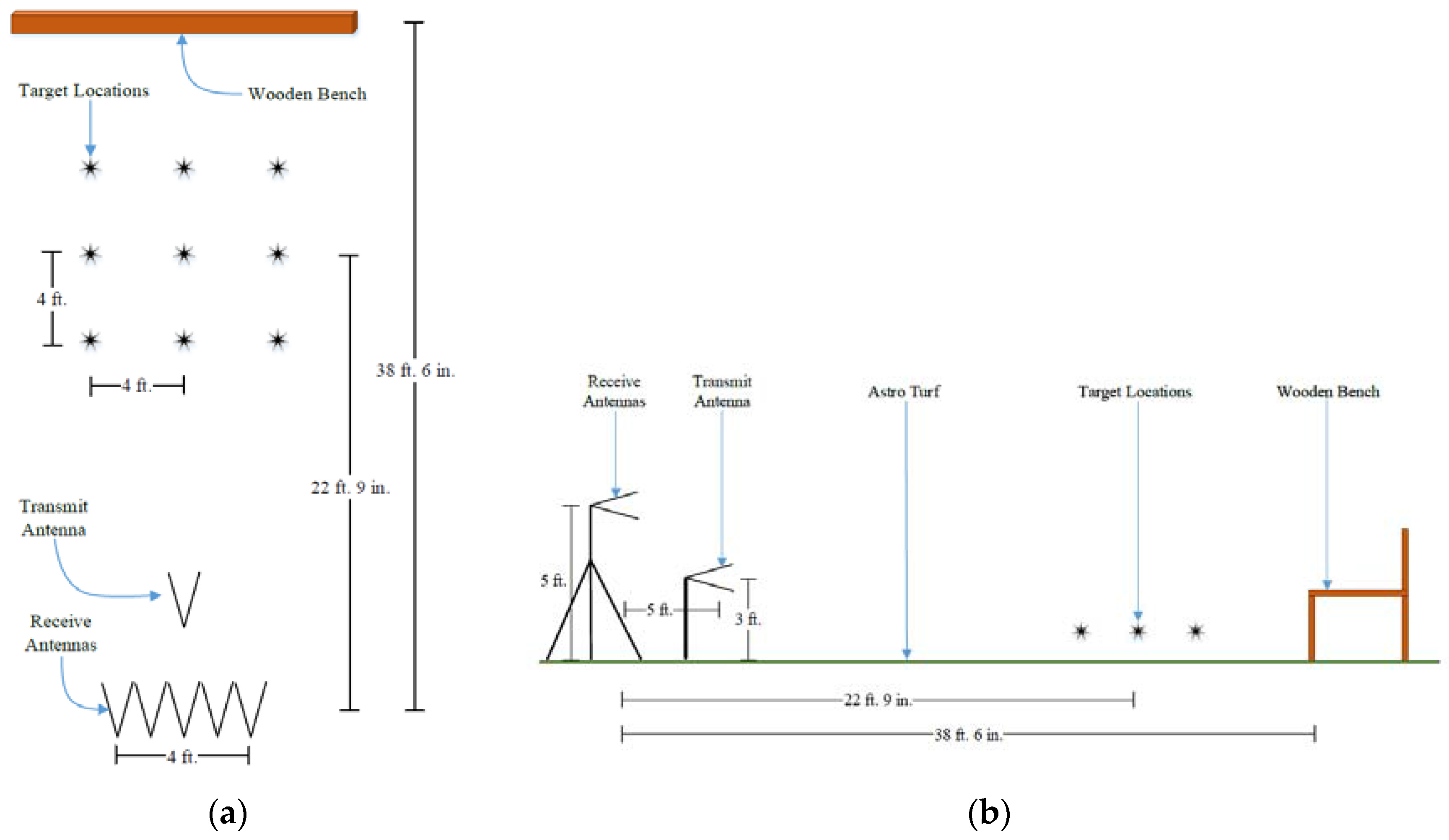
Data were collected with the targets positioned at nine different locations. The targets were placed at each location one at a time while data were collected. The targets were placed directly on the ground, thereby providing a more realistic scenario. Top down and side view diagrams of the SAR scene are illustrated in Figure 18.
All frequencies were transmitted and received on one antenna, before switching to the next antenna. The 16:1 switching network allowed for a SAR image to be collected every 20 min. In comparison, the same data collection using a moving aperture would take >2 h. The increased speed in data collection achieved by using a fixed aperture, however, comes at a cost. Since the time delay through each of the 16 channels is not exactly the same, a complex calibration matrix is needed during data processing, of size , where is the number of antennas and is the number of frequency steps.
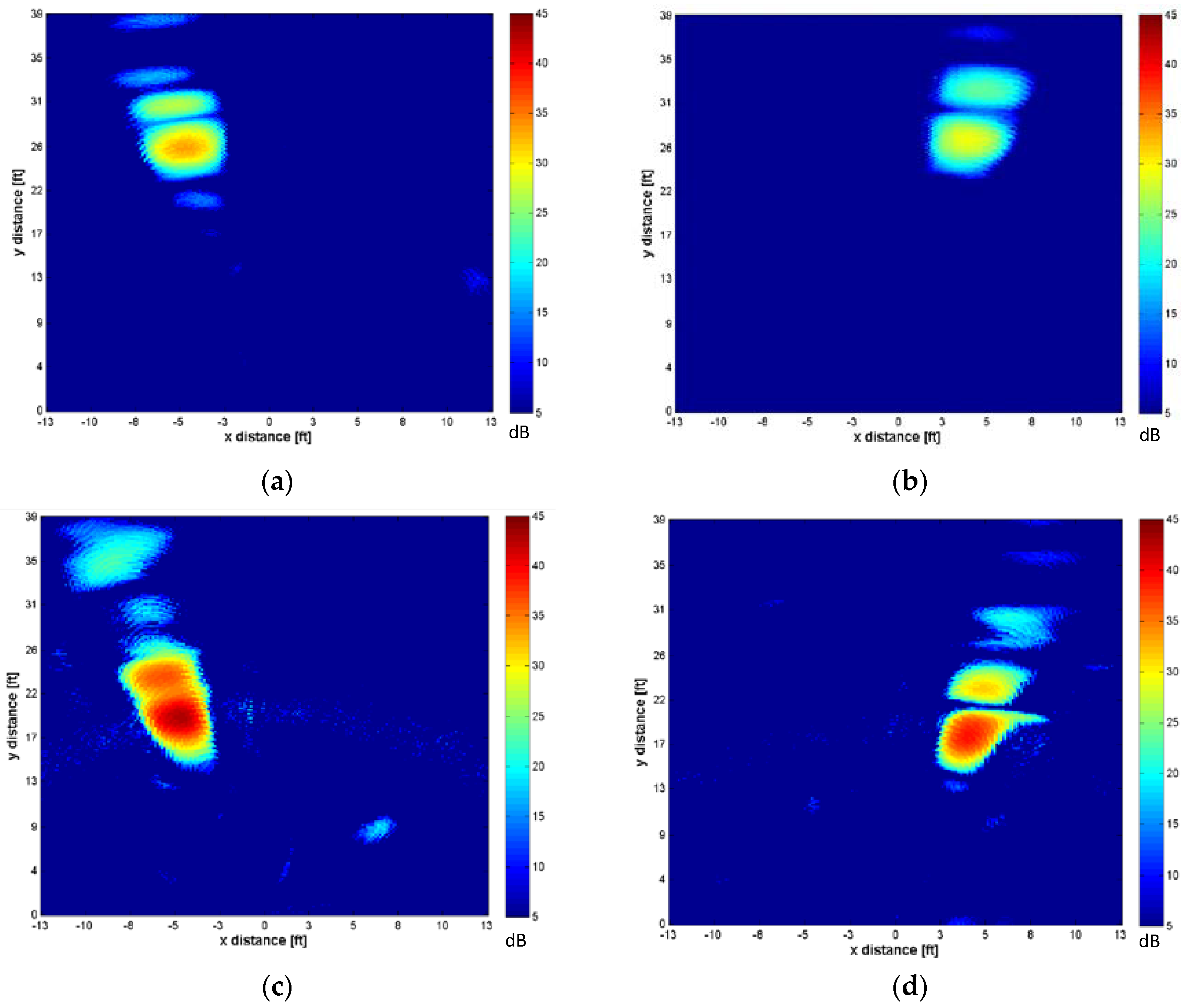
As an example, harmonic SAR images of Target 2 at four different locations are shown in in Figure 19.
5. Conclusions
This paper summarizes our results toward imaging of moving and stationary nonlinear targets using a harmonic radar. Our experimental results clearly illustrate the radar system’s capability of detecting a nonlinear target at a standoff range of at least 7.9 m (26 feet). The combined linear/nonlinear radar is able to separate linear targets from nonlinear targets and track both classes of targets in range and Doppler. Linear targets can be separated from stationary clutter with a minimum detectable velocity of approximately 1 m/s, if data are collected at 48 Hz. The nonlinear data collected show no visible antenna coupling or nonlinear clutter; thus, the minimum detectable velocity for the non-linear radar is 0 m/s. The natural clutter rejection properties of harmonic radar allows for detecting non-moving targets.
We also presented linear and harmonic synthetic aperture radar images collected from a moving aperture. We conclude from our results that harmonic radar data can be used to form high quality SAR images. These images show that a harmonic radar is able to ignore the strong linear response from a linear target, such as a corner reflector, and focus only on the nonlinear target.
Since our purpose was primarily to validate the theory of harmonic radar, the choice of frequency bands was made based on the availability of components in our laboratory and cost considerations. Under operational scenarios, one must take into account issues of frequency allocations and licenses/unlicensed bands. However, we believe that our validated concepts can work in any frequency range used.
We believe that our results provide the first published evidence of the use of harmonic radar for imaging nonlinear targets, both static and moving. Nonlinear radar is a viable technique for the detection of concealed electronic components containing semiconductors. Applications include detection of humans carrying cell phones buried under earthquake rubble and concealed eavesdropping devices carrying RF transmitters.
Acknowledgments
This research was supported by U.S. Army Research Office (ARO) Contract # W911NF-12-1-0305 through a subcontract from Delaware State University (DSU).
Author Contributions
All authors equally conceived and designed the experiments; K.A.G. performed the experiments; all authors analyzed the data; K.D.S. contributed the logistics and measurement facilities; R.M.N. wrote the first draft of the paper, and other authors contributed to its final form.
Dedication
This paper is dedicated to the memory of Marc Ressler of the U.S. Army Research Laboratory whose extensive experience in radar technology was taken advantage of during extensive discussions on the research.
Conflicts of Interest
The authors declare no conflict of interest. The funding sponsors had no role in the design of the study; in the collection, analyses, or interpretation of data; in the writing of the manuscript, and in the decision to publish the results.
References
- Faraday, M. Experimental Researches in Electricity; Dover Publications: New York, NY, USA, 1965; (Reprint). [Google Scholar]
- Shannon, C.E. A mathematical theory of communication. BSTJ 1948, 27, 379–423. [Google Scholar]
- Steer, M.B.; Khan, P.J. Large signal analysis of nonlinear microwave systems. In Proceedings of the IEEE MTT-S International Microwave Symposium Digest, San Francisco, CA, USA, 30 May–1 June 1984; pp. 402–403. [Google Scholar]
- Jakabosky, J.; Ryan, L.; Blunt, S. Transmitter-in-the-loop optimization of distorted OFDM radar emissions. In Proceedings of the IEEE Radar Conference, Ottawa, ON, Canada, 29 April–3 May 2013. [Google Scholar] [CrossRef]
- Tjora, S.; Lundheim, L. Distortion modeling and compensation in step frequency radars. IEEE Trans. Aerosp. Electron. Syst. 2012, 48, 360–374. [Google Scholar] [CrossRef]
- Wetherington, J.M.; Steer, M.B. Robust analog canceller for high-dynamic range radio frequency measurement. IEEE Trans. Microwave Theory Tech. 2012, 60, 1709–1719. [Google Scholar] [CrossRef]
- Bodson, M.; Sacks, A.; Khosla, P. Harmonic generation in adaptive feedforward cancellation schemes. IEEE Trans. Autom. Control 1994, 39, 1939–1944. [Google Scholar] [CrossRef]
- Pedro, J.C.; De Carvalho, N.B. Evaluating co-channel distortion ratio in microwave power amplifiers. IEEE Trans. Microwave Theory Tech. 2001, 49, 1777–1784. [Google Scholar] [CrossRef]
- Gallagher, K.A.; Mazzaro, G.J.; Narayanan, R.M.; Sherbondy, K.D.; Martone, A.F. Automated cancellation of harmonics using feed-forward filter reflection for radar transmitter linearization. In Proceedings of the SPIE Conference on Radar Sensor Technology XVIII, vol. 9077, Baltimore, MD, USA, 5–7 May 2014. [Google Scholar] [CrossRef]
- Gallagher, K.A.; Narayanan, R.M.; Mazzaro, G.J.; Sherbondy, K.D. Linearization of a harmonic radar transmitter by feed-forward filter reflection. In Proceedings of the IEEE Radar Conference, Cincinnati, OH, USA, 19–23 May 2014; pp. 1363–1368. [Google Scholar]
- Tellegen, B.D.H. Interaction between radio-waves? Nature 1933, 131, 840. [Google Scholar] [CrossRef]
- Bailey, V.A.; Martyn, D.F. Interaction of radio waves. Nature 1934, 133, 218. [Google Scholar] [CrossRef]
- Helme, B.G.M. Passive intermodulation of ICT components. In Proceedings of the IEE Colloquium on Screening Effectiveness Measurements (Ref. No. 1998/452), London, UK, 6 May 1998; pp. 1/1–1/8. [Google Scholar]
- Shitvov, A.; Schuchinsky, A.G.; Steer, M.B.; Wetherington, J.M. Characterisation of nonlinear distortion and intermodulation in passive devices and antennas. In Proceedings of the 8th European Conference on Antennas and Propagation (EuCAP 2014), The Hague, Netherlands, 6–11 April 2014; pp. 1454–1458. [Google Scholar]
- Golikov, V.; Hienonen, S.; Vainikainen, P. Passive intermodulation distortion measurements in mobile communication antennas. In Proceedings of the 54th IEEE Vehicular Technology Conference (VTC Fall 2001), Atlantic City, NJ, USA, 7–11 October 2001; pp. 2623–2625. [Google Scholar]
- Ranta, T.; Ella, J.; Pohjonen, H. Antenna switch linearity requirements for GSM/WCDMA mobile phone front-ends. In Proceedings of the European Conference on Wireless Technology, Paris, France, 3–4 Oct 2005; pp. 23–26. [Google Scholar]
- Moriya, A.; Inoue, M.; Kawachi, O. Development of high linearity duplexers with low passive intermodulation component. In Proceedings of the IEEE International Ultrasonics Symposium (IUS), Prague, Czech Republic, 21–25 July 2013; pp. 737–740. [Google Scholar]
- Wilkerson, J.R.; Gard, K.G.; Schuchinsky, A.G.; Steer, M.B. Electrothermal theory of intermodulation distortion in lossy microwave components. IEEE Trans. Microwave Theory Tech. 2008, 56, 2717–2725. [Google Scholar] [CrossRef]
- Opitz, C.L. Metal-detecting radar rejects clutter naturally. Microwaves 1976, 15, 12–14. [Google Scholar]
- Steele, D.W.; Rotondo, F.S.; Houck, J.L. Radar system for manmade device detection and discrimination from clutter. US Patent 7,830,299, 9 November 2010. [Google Scholar]
- Low, G.; Morissette, S.; Frazier, M. Junction range finder. U.S. Patent 3,732,567, 8 May 1973. [Google Scholar]
- Johnson, R.H. Metal target detection system. U.S. Patent 3,972,042, 27 July 1976. [Google Scholar]
- Opitz, C.L. Radar object detector using non-linearities. U.S. Patent 4,053,891, 11 October 1977. [Google Scholar]
- Danze, P.M.; Brienza, M.J. Radar target signature detector. U.S. Patent 5,191,343, 2 March 1993. [Google Scholar]
- Belyaev, V.V.; Mayunov, A.T.; Razin’kov, S.N. Effects of a metal-insulator-metal contact on the antenna in a radar monitoring system. Meas. Tech. 2001, 44, 871–875. [Google Scholar] [CrossRef]
- Belyaev, V.V.; Mayunov, A.T.; Razin’kov, S.N. Potential accuracy and resolving power of a nonlinear radar station with linear frequency modulation. Meas. Tech. 2003, 46, 698–701. [Google Scholar] [CrossRef]
- Belyaev, V.V.; Mayunov, A.T.; Razin’kov, S.N. Object detection range enhancement by means of nonlinear radar employing two signals with linear frequency modulation. Meas. Tech. 2003, 46, 802–805. [Google Scholar] [CrossRef]
- Khakimov, N.T. Recognition method of radio eavesdropping devices by radar sensing. Telecommun. Radio Eng. 2005, 63, 499–502. [Google Scholar] [CrossRef]
- Semyonov, E.V.; Semyonov, A.V. Applying the difference between the convolutions to investigate the nonlinearity of the transformation of test signals and object responses of ultrawideband signals. J. Commun. Technol. Electron. 2007, 52, 451–465. [Google Scholar] [CrossRef]
- Yakubov, V.P.; Shipilov, S.E.; Satarov, R.N.; Yurchenko, A.V. Remote ultra-wideband tomography of nonlinear electronic components. Tech. Phys. 2015, 60, 279–282. [Google Scholar] [CrossRef]
- Shefer, J.; Staras, H. Harmonic radar detecting and ranging system for automotive vehicles. U.S. Patent 3,781,879, 25 December 1973. [Google Scholar]
- Shefer, J.; Klensch, R.J.; Kaplan, G.; Johnson, H.C. Clutter-free radar for cars. Wireless World 1974, 80, 117–122. [Google Scholar]
- Shefer, J.; Klensch, R.J.; Kaplan, G.; Johnson, H.C. Clutter-free radar for cars – conclusion: frequency measurement and application. Wireless World 1974, 80, 199–202. [Google Scholar]
- Brazee, R.D.; Miller, E.S.; Reding, M.E.; Klein, M.G.; Nudd, B.; Zhu, H. A transponder for harmonic radar tracking of the black vine weevil in behavioral research. Trans. ASAE 2005, 48, 831–838. [Google Scholar] [CrossRef]
- O’Neal, M.E.; Landis, D.A.; Rothwell, E.; Kempel, L.; Reinhard, D. Tracking insects with harmonic radar: A case study. Am. Entomol. 2004, 50, 212–218. [Google Scholar] [CrossRef]
- Psychoudakis, D.; Moulder, W.; Chen, C.-C.; Zhu, H.; Volakis, J.L. A portable low-power harmonic radar system and conformal tag for insect tracking. IEEE Antennas Wireless Propag. Lett. 2008, 7, 444–447. [Google Scholar] [CrossRef]
- Aumann, H.; Kus, E.; Cline, B.; Emanetoglu, N. A low-cost harmonic radar for tracking very small tagged amphibians. In Proceedings of the International Instrumentation and Measurement Technology Conference (I2MTC), Minneapolis, MN, USA, 6–9 May 2013; pp. 234–237. [Google Scholar]
- Aumann, H.M.; Emanetoglu, N.W. A wideband harmonic radar for tracking small wood frogs. In Proceedings of the IEEE Radar Conference, Cincinnati, OH, USA, 19–23 May 2014; pp. 108–111. [Google Scholar]
- Gallagher, K.A. Harmonic Radar: Theory and Applications to Nonlinear Target Detection, Tracking, Imaging and Classification. Ph.D. Dissertation, The Pennsylvania State University, University Park, PA, USA, December 2015. [Google Scholar]
- Harger, R.O. Harmonic radar systems for near-ground in- foliage nonlinear scatterers. IEEE Trans. Aerosp. Electron. Syst. 1976, 12, 230–245. [Google Scholar]
- Powers, E.J.; Hong, J.Y.; Kim, Y.C. Cross sections and radar equation for nonlinear scatterers. IEEE Trans. Aerosp. Electron. Syst. 1981, 17, 602–605. [Google Scholar] [CrossRef]
- Bucci, O.M.; De Bonitatibus, A.; Pinto, I. Harmonic radar cross-section of bistatic nonlinear responder. Alta Freq. 1984, 53, 172–176. [Google Scholar]
- Shteĭnshleĭger, V.B. Nonlinear scattering of radio waves by metallic objects. Sov. Phys. Usp. 1984, 27, 60–68. [Google Scholar] [CrossRef]
- Powers, E.J.; Im, S. The utilization of higher-order spectra to determine nonlinear radar cross sections. In Proceedings of the IEEE International Conference on Acoustics, Speech, and Signal Processing (ICASSP-94), Adelaide, SA, Australia, 19–22 April 1994; pp. IV/437–IV/440. [Google Scholar]
- Shteinshleiger, V.B.; Misezhnikov, G.S.; Melnikov, L.Y. Study of the effect of nonlinear scattering of radio waves by real metallic objects. Record of the IEEE International Radar Conference, Alexandria, VA, USA, 8–11 May 1995; pp. 435–437. [Google Scholar]
- Vernigorov, N.S. Nonlinear transformation and scattering of an electromagnetic field by electrically nonlinear objects. J. Commun. Technol. Electron. 1997, 42, 1097–1101. [Google Scholar]
- Fazi, C.; Crowne, F.; Ressler, M. Design Considerations for Nonlinear Scattering; US Army Research Laboratory Technical Report ARL-TR-5684: Adelphi, MD, USA, September 2011. [Google Scholar]
- Fazi, C.; Crowne, F.; Ressler, M. Link budget calculations for nonlinear scattering. In Proceedings of the 6th European Conference on Antennas and Propagation (EUCAP), Prague, Czech Republic, 26–30 March 2012; pp. 1146–1150. [Google Scholar]
- Dardari, D. Detection and accurate localization of harmonic chipless tags. EURASIP J. Adv. Signal Process. 2015, 2015, 77. [Google Scholar] [CrossRef]
- Flemming, M.A.; Mullins, F.H.; Watson, A.W.D. Harmonic Radar Detection Systems. In Proceedings of the IEE International Conference on Radar (Radar-77), London, UK, 25–28 October 1977; pp. 552–554. [Google Scholar]
- Gallagher, K.A.; Mazzaro, G.J.; Martone, A.F.; Sherbondy, K.D.; Narayanan, R.M. Derivation and validation of the nonlinear radar range equation. In Proceedings of the SPIE Conference on Radar Sensor Technology XX, vol. 9829, Baltimore, MD, USA, 18–21 April 2016. [Google Scholar] [CrossRef]
- Gallagher, K.A.; Mazzaro, G.J.; Ranney, K.I.; Nguyen, L.H.; Sherbondy, K.D.; Narayanan, R.M. Nonlinear synthetic aperture radar imaging using a harmonic radar. In Proceedings of the SPIE Conference on Radar Sensor Technology XIX and Active and Passive Signatures VI, vol. 9461, Baltimore, MD, USA, 20–24 April 2015. [Google Scholar] [CrossRef]
- Stimson, G.W. Introduction to Airborne Radar, 2nd ed.; SciTech Publishing: Raleigh, NC, USA, 1998. [Google Scholar]
- Bruder, J.A. Measurement of the performance of moving target indication radars. In Proceedings of the IEEE Radar Conference, Arlington, VA, USA, 7–10 May 1990; pp. 170–175. [Google Scholar]
- Klemm, R. Introduction to space-time adaptive processing. Electron. Commun. Eng. J. 1999, 11, 5–12. [Google Scholar] [CrossRef]
- Mazzaro, G.J.; Martone, A.F.; McNamara, D.M. Detection of RF electronics by multitone harmonic radar. IEEE Trans. Aerosp. Electron. Syst. 2014, 50, 477–490. [Google Scholar] [CrossRef]
- Richards, M.A.; Scheer, J.A.; Holm, W.A. Principles of Modern Radar – Basic Principles; SciTech Publishing: Raleigh, NC, USA, 2010. [Google Scholar]
- Pilkay, G.L.; Reay-Jones, F.P.F.; Greene, J.K. Harmonic radar tagging for tracking movement of Nezara viridula (Hemiptera: Pentatomidae). Environ. Entomol. 2013, 42, 1020–1026. [Google Scholar] [CrossRef] [PubMed]
- Milanesio, D.; Saccani, M.; Maggiora, R.; Laurino, D.; Porporato, M. Design of an harmonic radar for the tracking of the Asian yellow-legged hornet. Ecol. Evol. 2016, 6, 2170–2178. [Google Scholar] [CrossRef] [PubMed]
- Chioukh, L.; Boutayeb, H.; Wu, K.; Deslandes, D. Monitoring vital signs using remote harmonic radar concept. In Proceedings of the 41st European Microwave Conference, Manchester, UK, 10–13 October 2011; pp. 1269–1272. [Google Scholar]
- Gallagher, K.A.; Narayanan, R.M.; Mazzaro, G.J.; Ranney, K.I.; Martone, A.F.; Sherbondy, K.D. Moving target indication with non-linear radar. In Proceedings of the IEEE Radar Conference, Arlington, VA, USA, 10–15 May 2015; pp. 1428–1433. [Google Scholar]
- Beane, E.F. Prediction of mixer intermodulation levels as function of local oscillator power. IEEE Trans. Electromagn. Compat. 1971, 13, 56–63. [Google Scholar] [CrossRef]
- Linnehan, R.; Schindler, J. Multistatic scattering from moving targets in multipath environments. In Proceedings of the IEEE Radar Conference, Pasadena, CA, USA, 4–8 May 2009. [Google Scholar] [CrossRef]
- Fitch, J.P. Synthetic Aperture Radar; Springer: New York, NY, USA, 1988. [Google Scholar]
- Davis, M.E.; Kapfer, R. Bistatic SAR using illumination from a tethered ground moving target indication radar. In Proceedings of the IEEE Radar Conference, Pasadena, CA, USA, 4–8 May 2009. [Google Scholar] [CrossRef]
- McCorkle, J.; Nguyen, L. Focusing of Dispersive Targets using Synthetic Aperture Radar; US Army Research Laboratory Technical Report ARL-TR-305: Adelphi, MD, USA, August 1994. [Google Scholar]
- Lim, D.; Xu, L.; Gianelli, C.; Li, J.; Nguyen, L.; Anderson, J. Time- and frequency-domain MIMO FLGPR imaging. In Proceedings of the IEEE Radar Conference, Arlington, VA, USA, 10–15 May 2015; pp. 1305–1310. [Google Scholar]
- Nguyen, L.; Koenig, F. Augmented reality for forward-looking synthetic aperture radar. In Proceedings of the IEEE Virtual Reality Short Papers and Posters, Costa Mesa, CA, USA, 4–8 March 2012; pp. 145–146. [Google Scholar]
- Ahmad, F.; Amin, M.G.; Kassam, S.A. Synthetic aperture beamformer for imaging through a dielectric wall. IEEE Trans. Aerosp. Electron. Syst. 2005, 41, 271–283. [Google Scholar] [CrossRef]
- Dogaru, T.; Le, C.; Nguyen, L. Synthetic Aperture Radar Images of a Simple Room Based on Computer Models; US Army Research Laboratory Technical Report ARL-TR-5193: Adelphi, MD, USA, May 2010. [Google Scholar]
- Berger, T.; Hamran, S.-E. Harmonic synthetic aperture radar processing. IEEE Geosci. Remote Sens. Lett. 2015, 12, 2066–2069. [Google Scholar] [CrossRef]
Figure 1.
Block diagram showing a radar signal path.
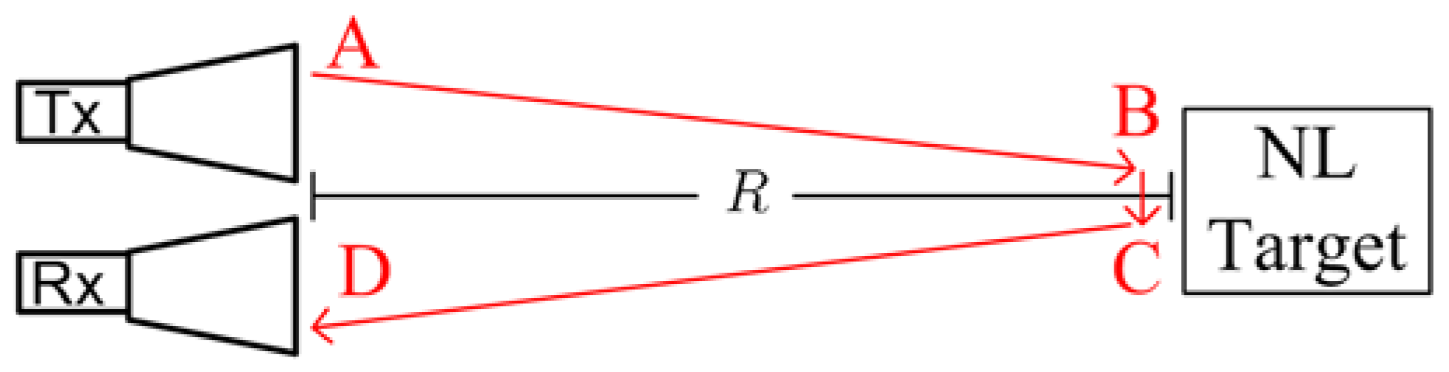
Figure 2.
Block diagram of the harmonic radar system.
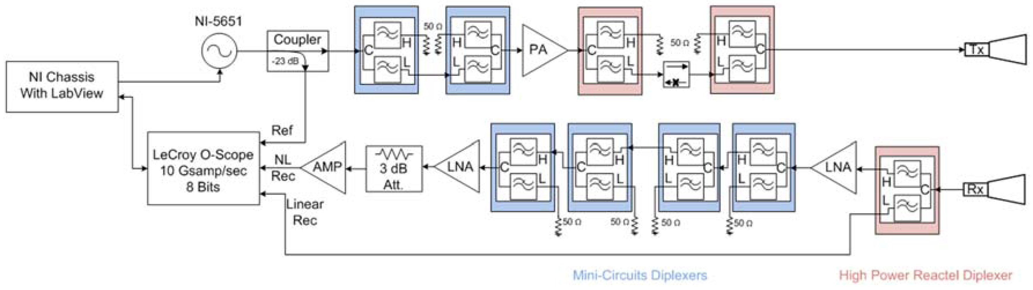
Figure 3.
Transforming the raw frequency domain data to the range domain.
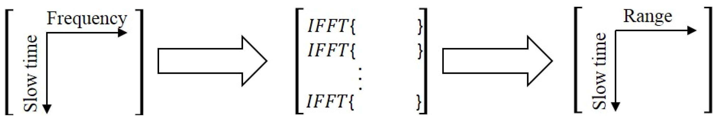
Figure 4.
Transforming the slow time domain to the Doppler speed domain.
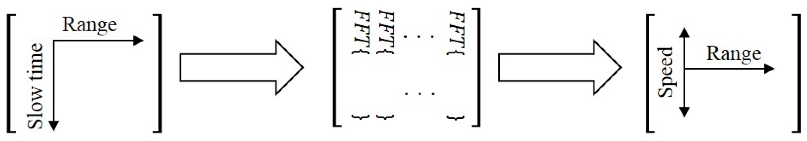
Figure 5.
(a) Test setup for moving target imaging; (b) Photograph of the nonlinear target constructed.
Figure 5.
(a) Test setup for moving target imaging; (b) Photograph of the nonlinear target constructed.
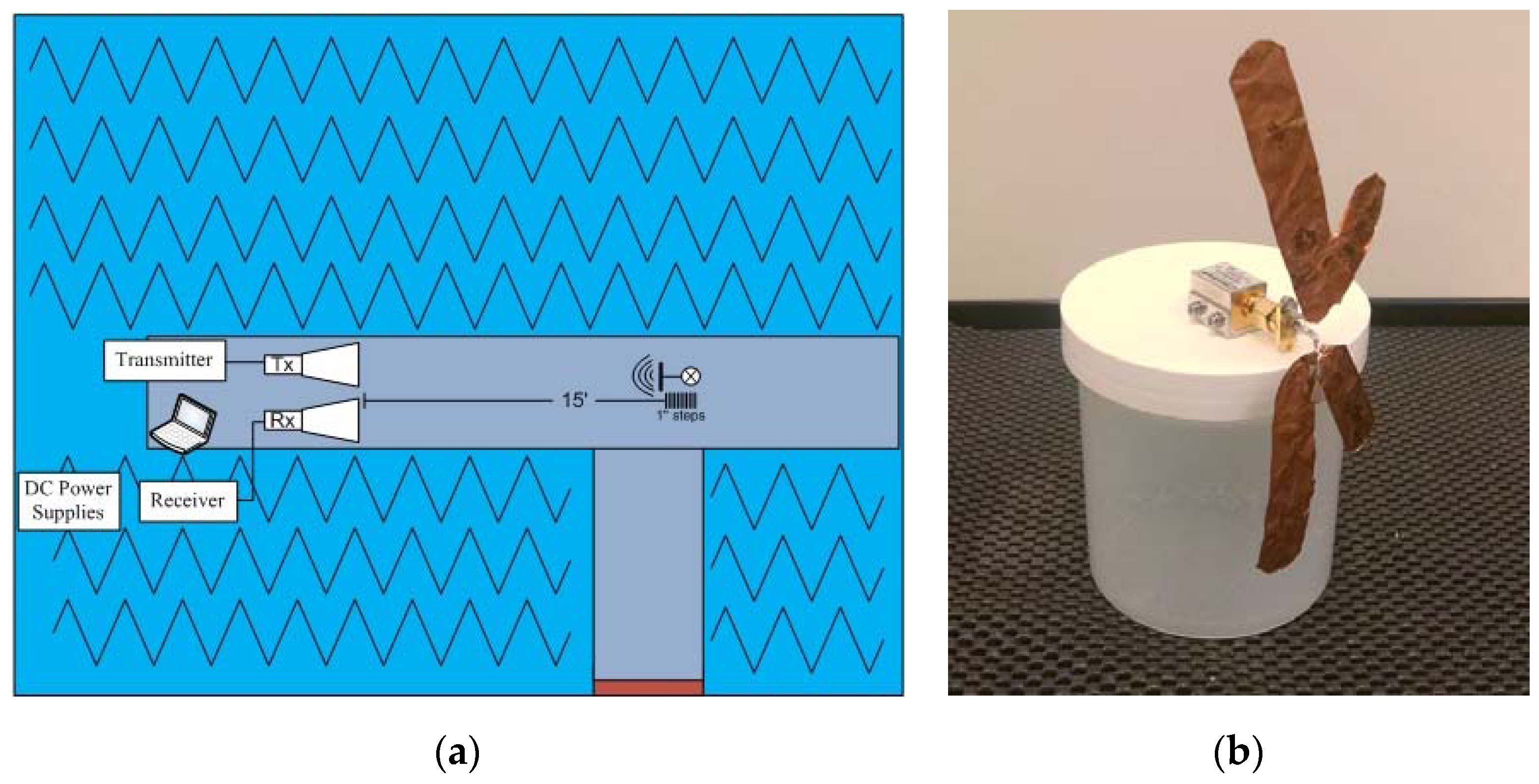
Figure 6.
Photographs of the test setup: (a) Radar transmitter; (b) Radar antennas; (c) Radar receiver.
Figure 6.
Photographs of the test setup: (a) Radar transmitter; (b) Radar antennas; (c) Radar receiver.
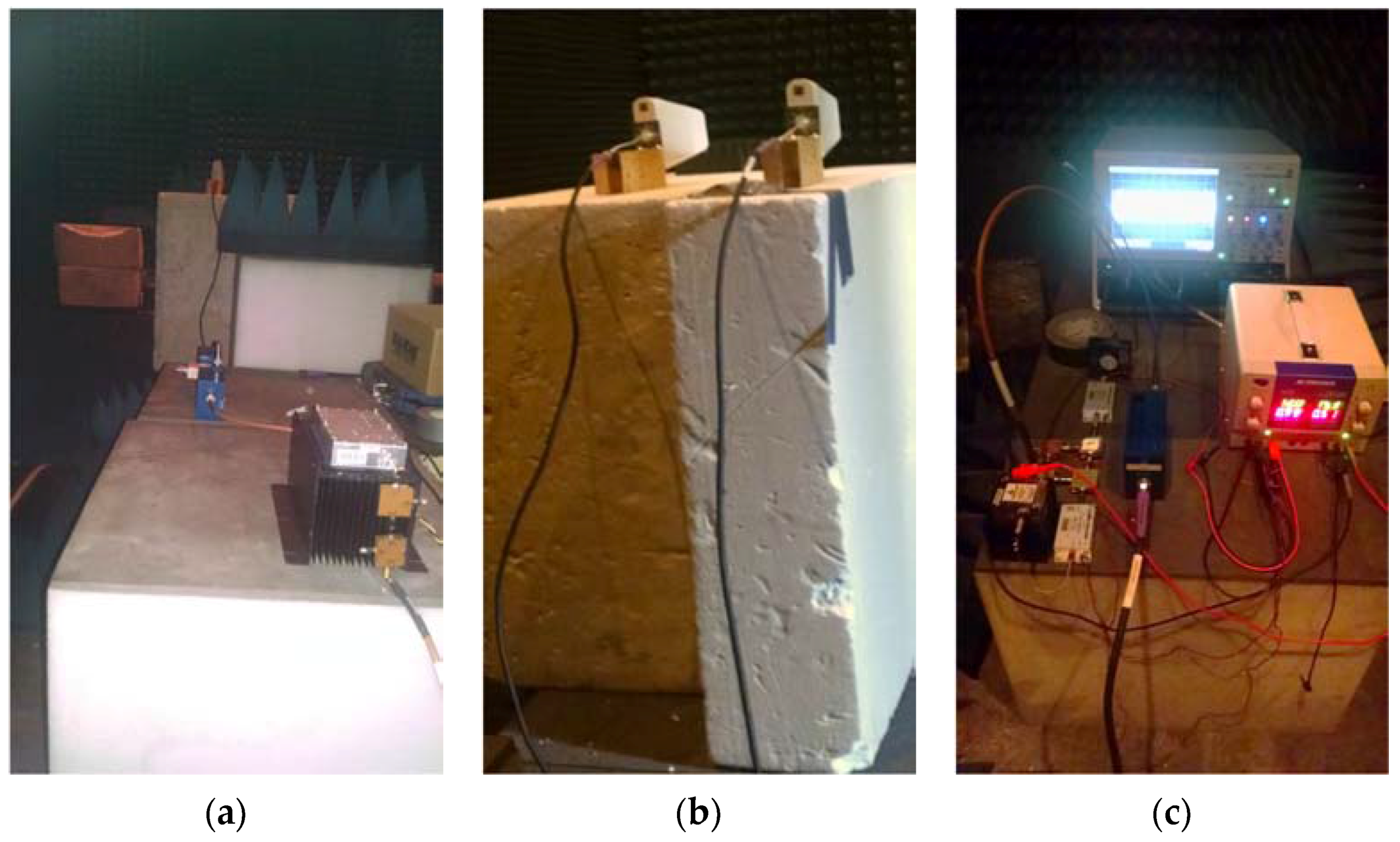
Figure 7.
Range-Doppler plots of the nonlinear moving target at: (a) Fundamental frequency; (b) Harmonic frequency.
Figure 7.
Range-Doppler plots of the nonlinear moving target at: (a) Fundamental frequency; (b) Harmonic frequency.
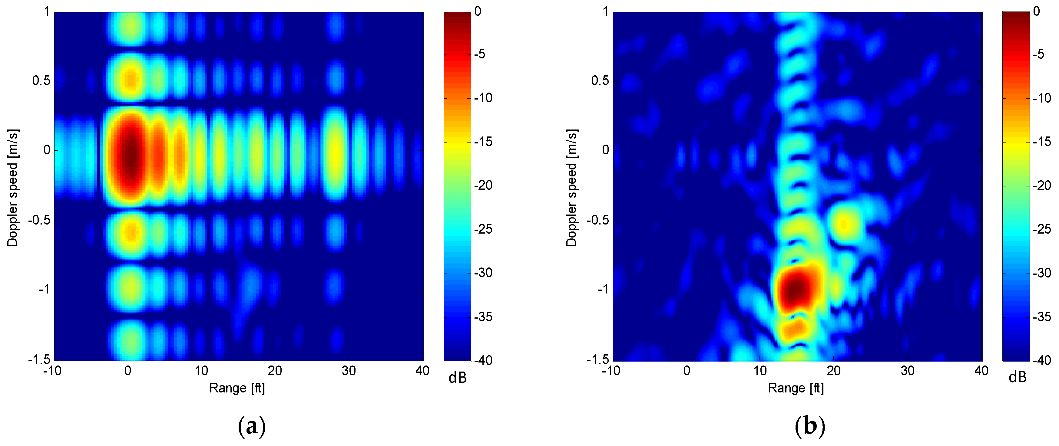
Figure 8.
Range-Doppler plots of the nonlinear moving target with Hamming window applied at: (a) Fundamental frequency; (b) Harmonic frequency.
Figure 8.
Range-Doppler plots of the nonlinear moving target with Hamming window applied at: (a) Fundamental frequency; (b) Harmonic frequency.

Figure 9.
Explanation of Figure 8 features for: (a) Fundamental frequency; (b) Harmonic frequency.
Figure 9.
Explanation of Figure 8 features for: (a) Fundamental frequency; (b) Harmonic frequency.
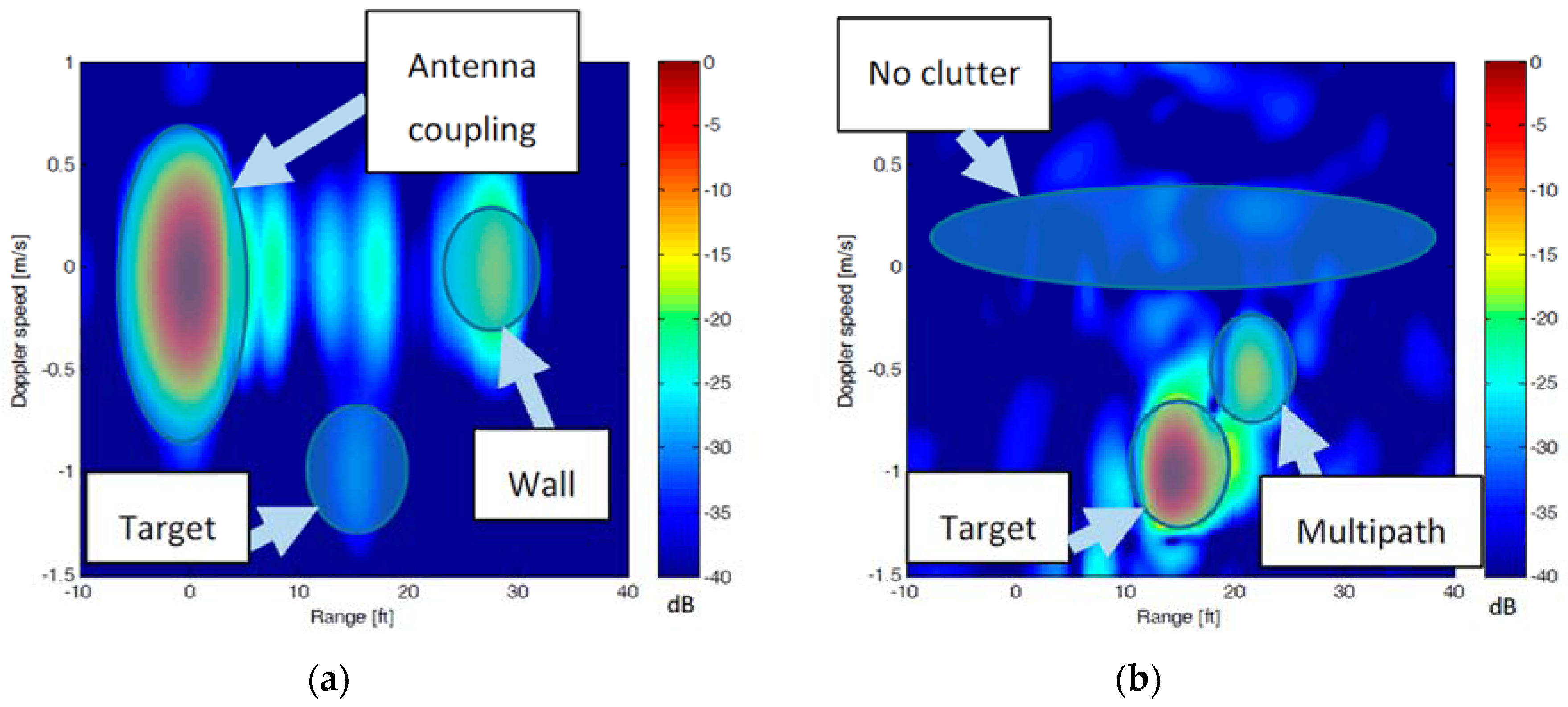
Figure 10.
Geometry of synthetic aperture radar (SAR) imaging scene.

Figure 11.
Test setup for moving aperture SAR imaging.

Figure 12.
Photographs of the harmonic SAR system.

Figure 13.
Photographs of the antennas mounted on the plastic cart and the duct tape track.
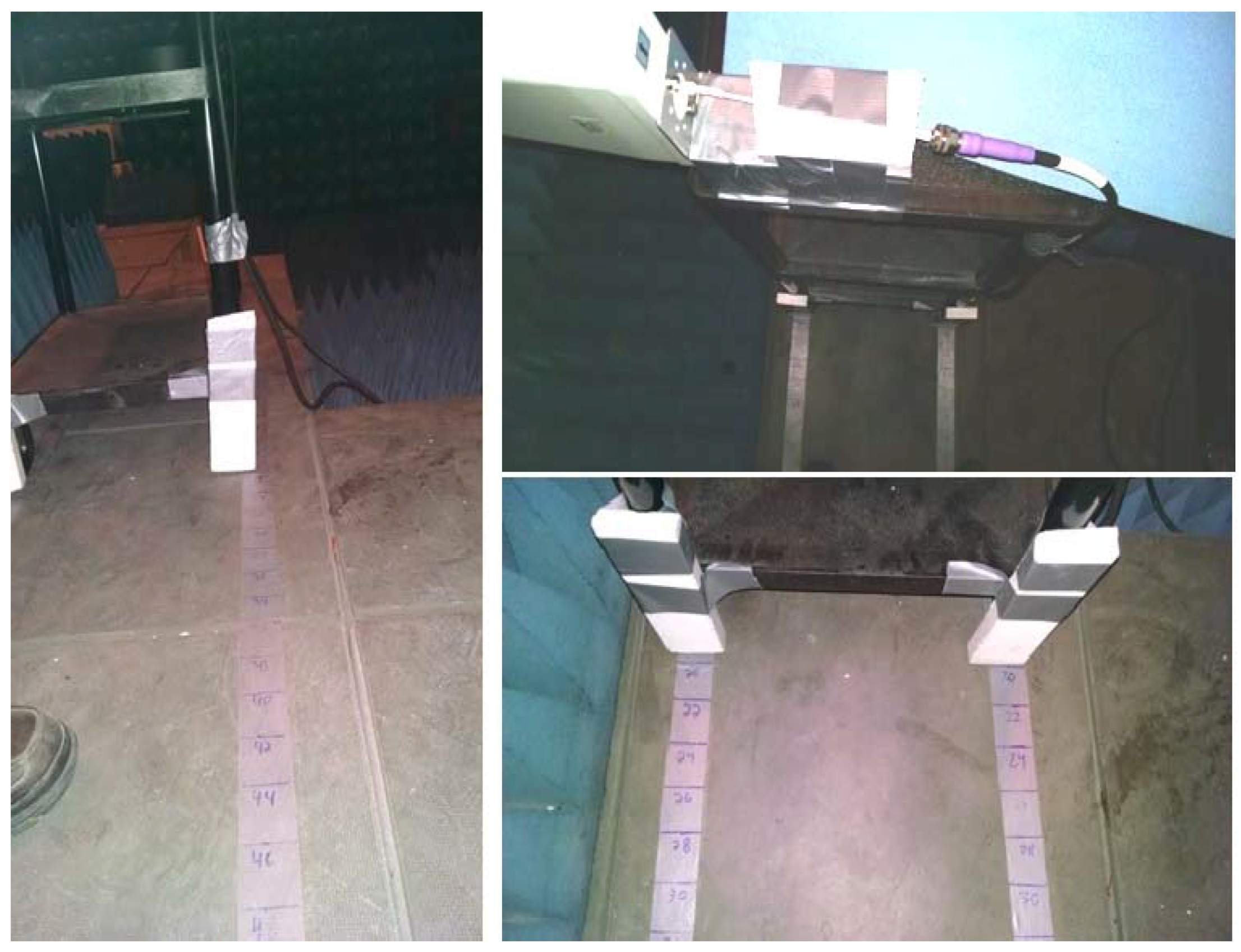
Figure 14.
Photographs of the targets used for SAR imaging: (a) Linear target; (b) Nonlinear target.
Figure 14.
Photographs of the targets used for SAR imaging: (a) Linear target; (b) Nonlinear target.

Figure 15.
SAR results from the nonlinear target at position A and the linear target at position B: (a) Linear SAR image; (b) Harmonic SAR image.
Figure 15.
SAR results from the nonlinear target at position A and the linear target at position B: (a) Linear SAR image; (b) Harmonic SAR image.

Figure 16.
Explanation of Figure 15 features for: (a) Fundamental frequency; (b) Harmonic frequency.
Figure 16.
Explanation of Figure 15 features for: (a) Fundamental frequency; (b) Harmonic frequency.
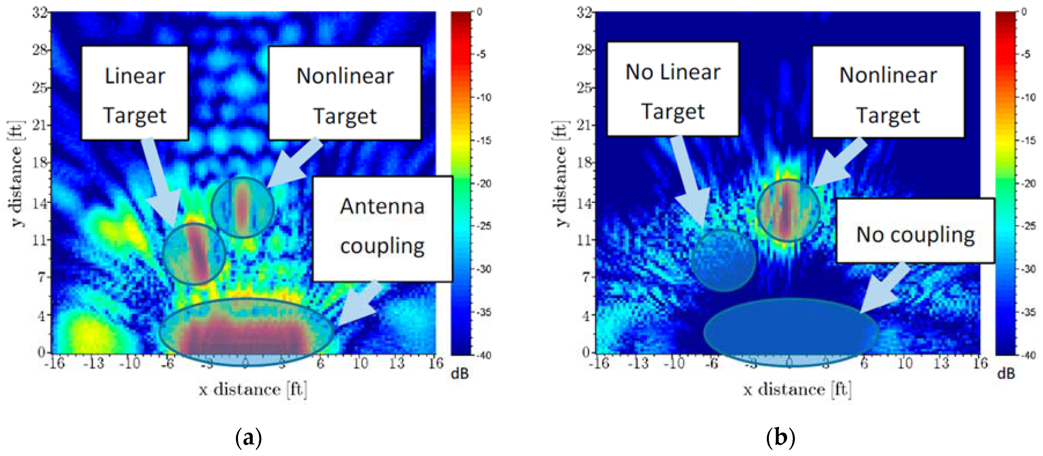
Figure 17.
Photograph of the 16-antenna array used to collect SAR images.
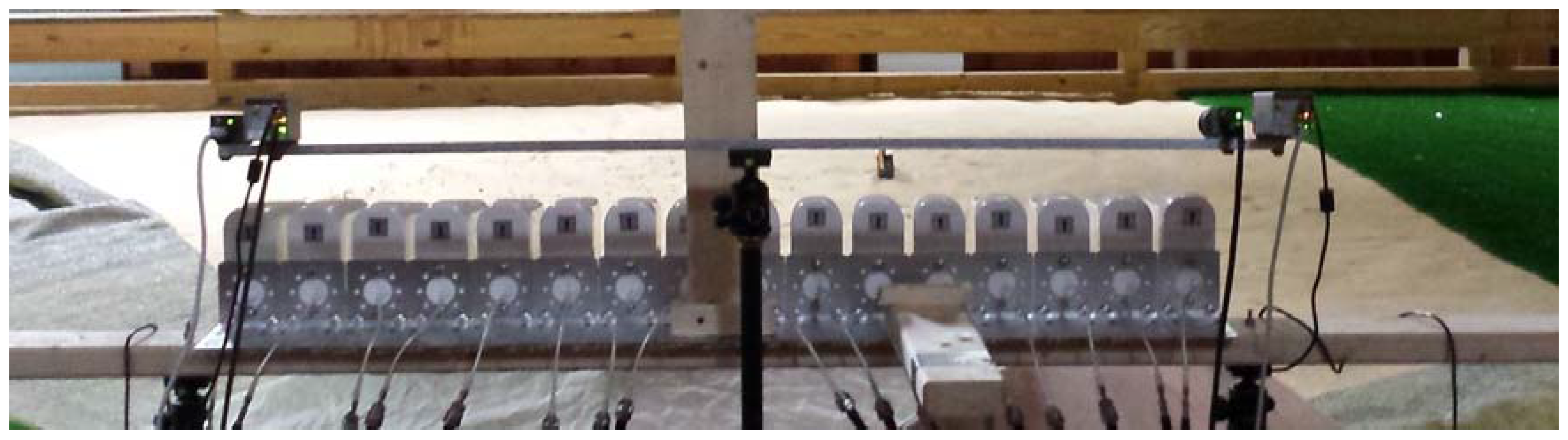
Figure 18.
Geometry of the scene used for SAR imaging. (a) Top view; (b) Side view.

Figure 19.
SAR images of Target 2 at different locations in the scene: (a) at x = −1.22 m = −4 feet, y = 7.92 m = 26 feet; (b) at x = 1.22 m = 4 feet, y = 7.92 m = 26 feet; (c) at x = −1.22 m = −4 feet, y = 5.79 m = 19 feet; (d) at x = −1.22 m = −4 feet, y = 5.79 m = 19 feet.
Figure 19.
SAR images of Target 2 at different locations in the scene: (a) at x = −1.22 m = −4 feet, y = 7.92 m = 26 feet; (b) at x = 1.22 m = 4 feet, y = 7.92 m = 26 feet; (c) at x = −1.22 m = −4 feet, y = 5.79 m = 19 feet; (d) at x = −1.22 m = −4 feet, y = 5.79 m = 19 feet.


Table 1.
Specifications of the radar system.
| Parameter | Value |
|---|---|
| Linear frequency range | 800–1000 MHz |
| Harmonic frequency range | 1.6–2 GHz |
| Transmit power | +40 dBm |
| Transmit antenna gain at fundamental | 10 dBi |
| Receive antenna gain at fundamental | 10 dBi |
| Receive antenna gain at second harmonic | 8 dBi |
| Range resolution at fundamental | 75 cm (2.46 feet) |
| Range resolution at second harmonic | 37.5 cm (1.23 feet) |
| System noise floor | −125 dBm |
Table 2.
x- and y-coordinates of target positions.
| Position | x-Coordinate (m/ft) | y-Coordinate (m/ft) |
|---|---|---|
| A | 0/0 | 4.57/15 |
| B | −0.91/−3 | 3.66/12 |
Table 3.
Target Descriptions for Switched Aperture SAR Imaging.
| Target | Description |
|---|---|
| 1 | Hand Held Radio 1 |
| 2 | Hand Held Radio 2 |
| 3 | Hand Held Radio 3 |
| 4 | Commercial RF amplifier, powered on using batteries |
| 5 | Commercial RF amplifier, no power |
© 2017 by the authors. Licensee MDPI, Basel, Switzerland. This article is an open access article distributed under the terms and conditions of the Creative Commons Attribution (CC BY) license (http://creativecommons.org/licenses/by/4.0/).
Share and Cite
MDPI and ACS Style
Gallagher, K.A.; Narayanan, R.M.; Mazzaro, G.J.; Martone, A.F.; Sherbondy, K.D. Static and Moving Target Imaging Using Harmonic Radar. Electronics 2017, 6, 30. https://doi.org/10.3390/electronics6020030
AMA Style
Gallagher KA, Narayanan RM, Mazzaro GJ, Martone AF, Sherbondy KD. Static and Moving Target Imaging Using Harmonic Radar. Electronics. 2017; 6(2):30. https://doi.org/10.3390/electronics6020030
Chicago/Turabian StyleGallagher, Kyle A., Ram M. Narayanan, Gregory J. Mazzaro, Anthony F. Martone, and Kelly D. Sherbondy. 2017. "Static and Moving Target Imaging Using Harmonic Radar" Electronics 6, no. 2: 30. https://doi.org/10.3390/electronics6020030
Note that from the first issue of 2016, this journal uses article numbers instead of page numbers. See further details here.