Subsecond Tsunamis and Delays in Decentralized Electronic Systems
by
Pedro D. Manrique
1, 
Minzhang Zheng
1,
Zhenfeng Cao
1,
David Dylan Johnson Restrepo
1,
Pak Ming Hui
2 and
Neil F. Johnson
1,* 1
Complex Systems Initiative, Physics Department, University of Miami, Coral Gables, FL 33126, USA
2
Department of Physics, Chinese University of Hong Kong, Shatin, Hong Kong SAR, China
*
Author to whom correspondence should be addressed.
Electronics 2017, 6(4), 80; https://doi.org/10.3390/electronics6040080
Submission received: 1 September 2017
/
Revised: 21 September 2017
/
Accepted: 30 September 2017
/
Published: 11 October 2017
Abstract
:Driven by technological advances and economic gain, society’s electronic systems are becoming larger, faster, more decentralized and autonomous, and yet with increasing global reach. A prime example are the networks of financial markets which—in contrast to popular perception—are largely all-electronic and decentralized with no top-down real-time controller. This prototypical system generates complex subsecond dynamics that emerge from a decentralized network comprising heterogeneous hardware and software components, communications links, and a diverse ecology of trading algorithms that operate and compete within this all-electronics environment. Indeed, these same technological and economic drivers are likely to generate a similarly competitive all-electronic ecology in a variety of future cyberphysical domains such as e-commerce, defense and the transportation system, including the likely appearance of large numbers of autonomous vehicles on the streets of many cities. Hence there is an urgent need to deepen our understanding of stability, safety and security across a wide range of ultrafast, large, decentralized all-electronic systems—in short, society will eventually need to understand what extreme behaviors can occur, why, and what might be the impact of both intentional and unintentional system perturbations. Here we set out a framework for addressing this issue, using a generic model of heterogeneous, adaptive, autonomous components where each has a realistic limit on the amount of information and processing power available to it. We focus on the specific impact of delayed information, possibly through an accidental shift in the latency of information transmission, or an intentional attack from the outside. While much remains to be done in terms of developing formal mathematical results for this system, our preliminary results indicate the type of impact that can occur and the structure of a mathematical theory which may eventually describe it.
Keywords:
electronics; complex systems; computation; ultra-fast networks; competition; modeling; latency1. Introduction
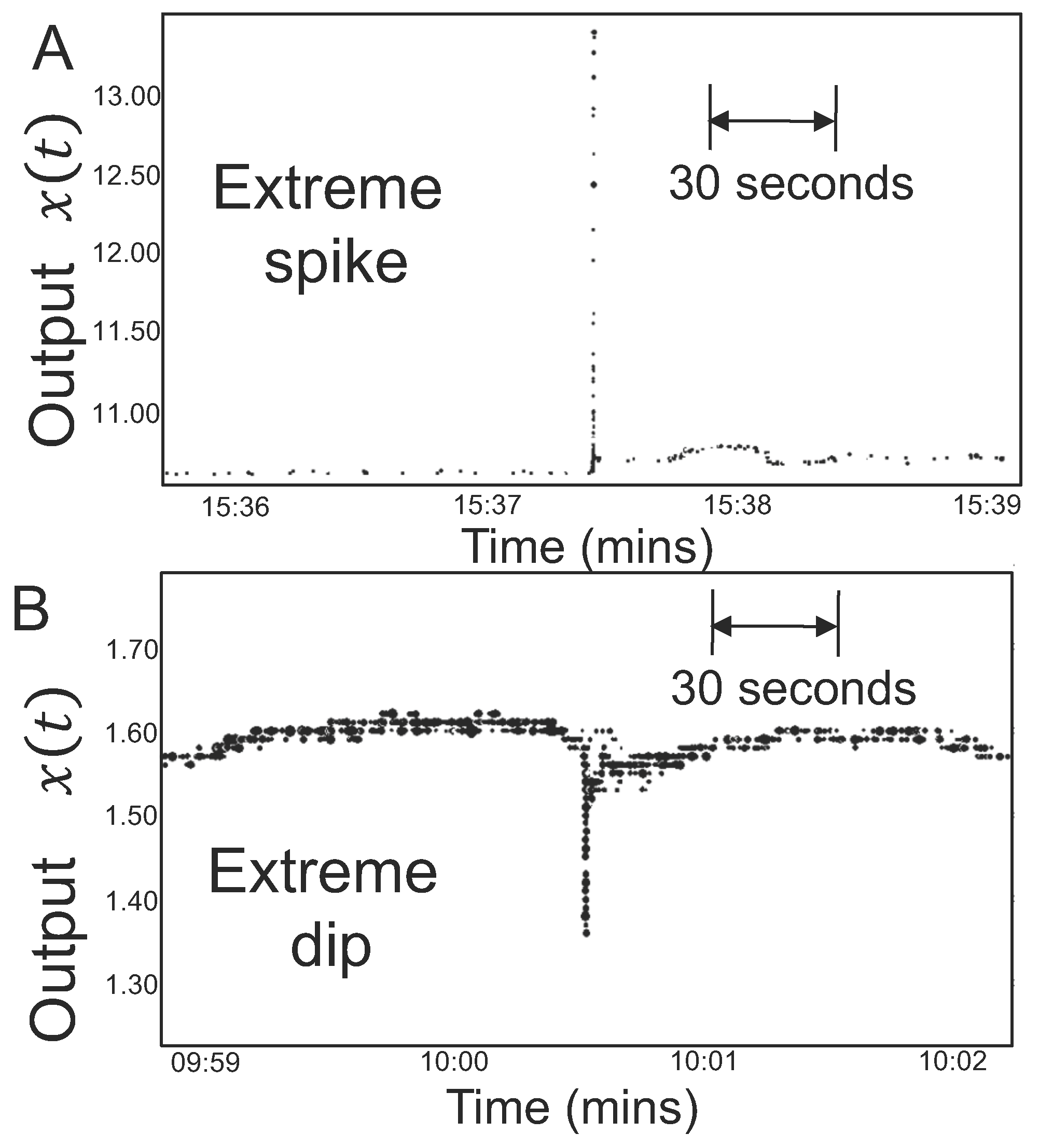
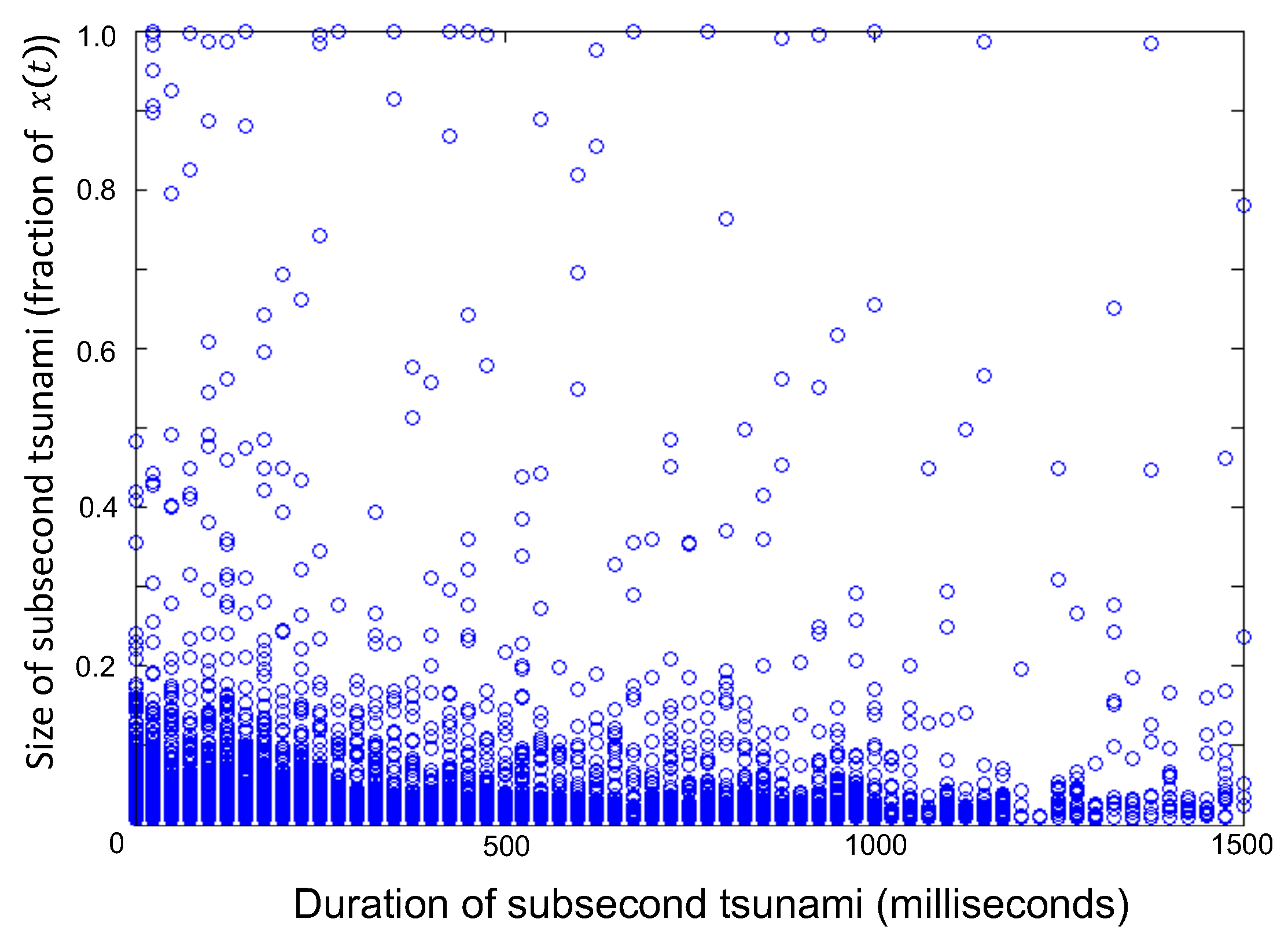
The recent technological advances in the speed and processing power of electronic components, are fueling a drive towards increased automation and global reach of society’s cyberphysical systems [1,2]. Since these systems operate in a free market economy in most countries, and each component almost by definition is looking to win, this means that such systems can be regarded as a heterogeneous collection of competitive components that operate as an ecology driven by survival of the fittest [1,2,3,4,5,6,7,8,9]. This leaves regulators with the significant problem of understanding what might go wrong at the system level, and how to prevent it. An ideal example of such a system is the decentralized network of electronic financial exchanges that has grown up across the globe. The resulting system comprises a heterogeneous, decentralized collection of adaptive, autonomous components (e.g., trading platforms and hard-wired logic gates) where each has limited information about the overall system and limited processing power [10,11,12,13]. Such financial market systems operate down to the microsecond timescale beyond human reaction times, and hence may serve as a proxy for any other all-electronic, decentralized system comprising an ecology of hardware and software components, network links, and underlying algorithms which compete to make a profit [10,11,12,13]. Figure 1 shows two examples of the type of subsecond tsunami (i.e., extreme behaviors) that have been observed in the real all-electronic exchange data (see Ref. [14] for more details). Both are more than 30 standard deviations larger than the average price movement either side of an event and so are very unlikely to have arisen by chance. During the period of study of approximately five years, we found 18,520 such ultrafast dips and spikes. Figure 2 shows a plot of their sizes and durations. There is therefore an urgent need to deepen our understanding of the stability of such decentralized electronic systems. In particular, the stability and safety of such systems will rely on understanding what extreme behaviors can occur, why, and what might be the impact of both intentional and unintentional system perturbations.
In this paper, we present a discussion of this topic based on a combination of a generic, binary model of heterogeneous, adaptive, autonomous objects with limited information and processing power, and recent subsecond data from these decentralized, all-electronic financial market exchanges. We focus on the important problem of how delayed information in such systems impacts their overall stability, in particular the appearance of sudden large changes at the system level akin to subsecond tsunamis. Such delayed information can arise either through poor individual information processing, an accidental shift in the latency of information transmission, or an intentional attack from the outside [10,11,12,13]. Much remains to be done in terms of developing formal mathematical results for this system, hence this paper should be seen as laying out a framework as opposed to solving this problem. However our preliminary results already show the type of impacts that can occur—in particular, in relation to the extreme subsecond shifts (tsunamis) which have been observed in financial market data. Such subsecond tsunamis are relatively frequent (Figure 1 and Figure 2) and yet are still not well understood. More generally, this topic of decentralized societal networks, in particular those based on financial activity, touches on a wide range of areas of interest to the electronics community, including communications and information processing, microwave and electronic system engineering, systems and control engineering.
The current work builds on the introduction provided by Ref. [15], but goes well beyond Ref. [15] by providing (1) analysis of the magnitude (i.e., severity) of an extreme event under the influence of information delays (i.e., latency); (2) analysis of the role of the confidence threshold in enhancing or suppressing latency effects on single-node extreme events; (3) inclusion of results from a null model in which each agent uses an uncorrelated decision-making mechanism, and an analysis of how the actual effects differ from the results of this null model; (4) the setting up of an analytic framework to study the system using a quasi-deterministic approach; and (5) the presentation of actual stock trade data that illustrate the extraordinary variety of subsecond extreme events that arise in the real world.
We start by giving some background to the problem (Section 2). Then we present the generic model which, we stress, is a first attempt to conceptualize the problem and open it up to quantitative analysis (Section 3). Section 4 contains results from the simulation of the model, while Section 5 gives some analytical analysis of the model. In Section 6 we provide real world examples of subsecond extreme events in stock trade data. Section 7 provides Conclusions.
2. Background
The practical problem of having a large-scale system upon which society depends, but which operates down to microsecond timescales and beyond, is trivial to deduce but has highly non-trivial implications: specifically, it becomes impossible for any human to be able to detect extreme unwanted behavior on that timescale in real time, and then step in to stop it. This is because the human response time for taking in information and then taking an action, is of the order of a second [12] and there are one million microseconds in one second. Modern financial markets only have one physical limitation in principle: the finite speed of light. Hence any technological advantages that enable one component (e.g., financial entity, and hence their electronic hardware and connectivity) to gain access to information more quickly, will be exploited. This has driven a race toward zero latency, limited only by the finite speed of light and the finite duration of the underlying physical processes in the various electronic components [10,11,12,13]. High-speed servers, and ultimately algorithms, continually take in and process information on the scale of microseconds. Most importantly, this is predicted to be reduced even further in the near future due to new hard-wired semiconductor technology [10].
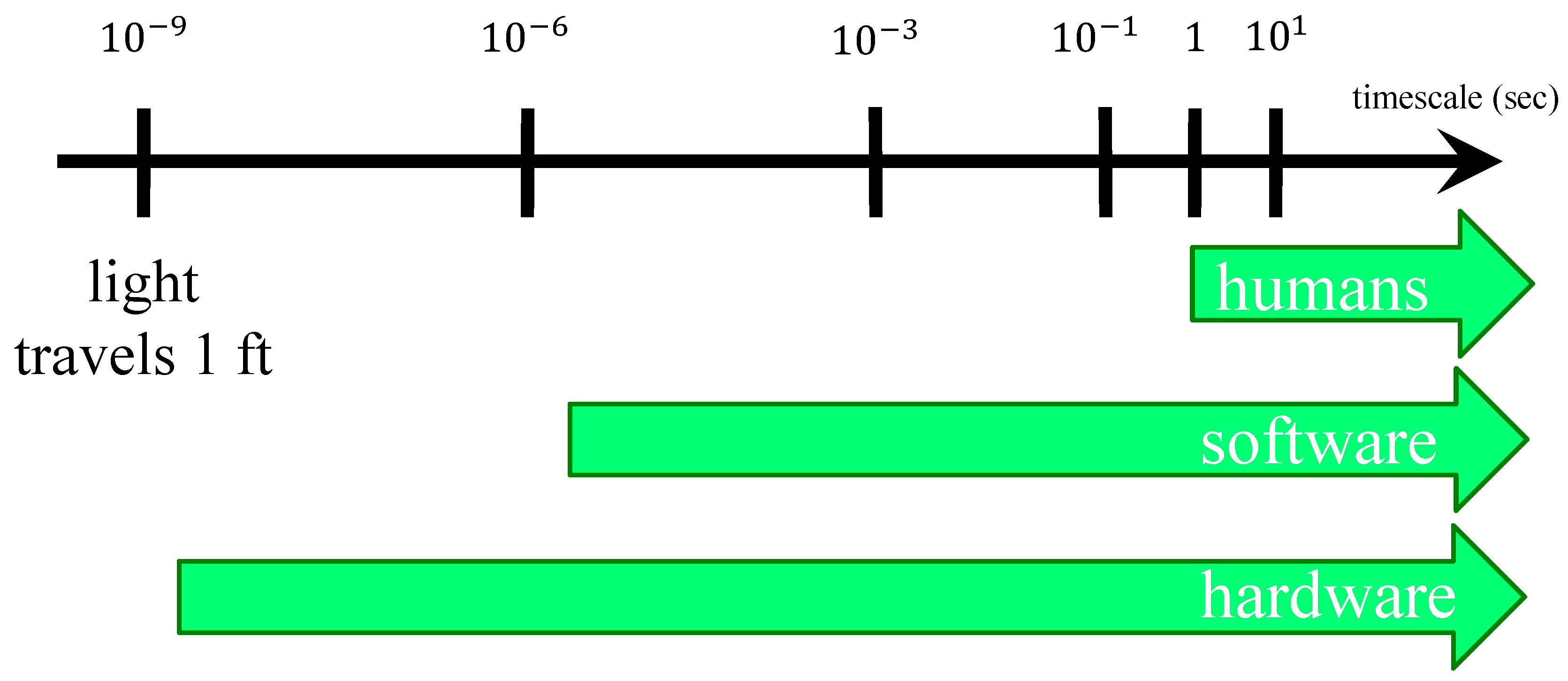
Figure 3 illustrates the problem more explicitly. There is a broad range of timescales between the nanosecond scale during which any form of electromagnetic radiation, including light and microwaves, will travel 1 foot in free space, and the second scale on which humans can operate. With typical electronic hardware therefore in principle operating down toward the nanosecond scale, and software systems operating down toward the microsecond scale, there is a huge regime of timescales (– s) in which rules, regulations and hence laws need to be applied but where the basic dynamics of collective behavior is little understood. Specifically, though each component and algorithm may be reasonably well calibrated, the collective behavior can show emergent properties, just as the collective behavior of cars (e.g., traffic jams) does not follow directly from understanding the mechanics of any single vehicle [16].
This interest in such complex systems is not just academic. Indeed, the question of what happens when for example a delay is added to the information (i.e., latency) has taken on high commercial, legal and political importance following regulators allowing a 350 microsecond delay to be intentionally introduced into one these financial exchanges. The difficulty that regulators had in taking such a decision, rests on the fact that this is a complex dynamical network system and there is a lack of mathematically tractable models for such a population of competing, heterogeneous, adaptive components. To make matters worse for regulators, substantial amounts of money and engineering effort are being put into increasing data acquisition speeds, e.g., through the building of transatlantic cables to shave milliseconds from the transfer time of financial data between London and New York [11]; through new global networks of microwave communication towers; and through new hard-wired semiconductor technology to reduce decision-making times toward the nanosecond scale [10]. Indeed, this decision by U.S. regulators to allow the Investors Exchange (IEX) group to add this intentional 350 microsecond delay ( s), has spawned similar request by other nodes in the exchange network. The IEX speed-bump is implemented by means of an additional 38 m coil of fiber-optic cable that has been added within the electronics of their exchange network [13]. While 350 microsecond seems insignificant when compared to the 2010 ‘Flash Crash’ which lasted ∼ s [17], current market conditions regularly see hundreds of orders executed electronically within one millisecond. Furthermore, there is now a looming need to quantify the impact of such systematic delays in more general complex systems. e.g., the swarms of self-driving cars that are likely to be on the streets of many cities within a decade, with each competing for bandwidth [18,19]. Similar competitive, decentralized scenarios are also likely for autonomous drones at some stage in the future [20] as well as other sociotechnical systems [21]. These considerations raise the following important questions that we explore in this paper, regarding what extreme behaviors emerge from such systems; what will the effect be of intended but also accidental delays; and what steps could be taken to mitigate such effects. By way of note, it does not seem to be a coincidence that similar issues surround our current limited understanding of the human brain which is arguably the most complex decentralized network that exists [22].
3. Model
The model that we consider in this paper is shown in schematic form in Figure 4. It is of course incomplete; it makes multiple assumptions; and there are many possible variants. However it captures some of the essential features that are of interest in complex, decentralized electronic systems: there is a population of heterogeneous, autonomous components (agents) who repeatedly act based on some limited global information that is fed back to them, where this information is the recent history of system outcomes that they collectively produced in previous recent timesteps. Each component (agent) has only limited information processing capabilities and there is no inter-agent communication. At the very least, this gives us a well-defined system for simulating and also for mathematical analysis. Of particular interest in this paper, it allows us to add a temporal perturbation in terms of a delay in the common information which is fed to each component concerning prior global outcomes. The resulting Delayed Grand Canonical Minority Game (DGCMG) therefore represents a non-trivial generalization of the Grand Canonical Minority Game (GCMG) introduced in 1999 [23,24,25,26]. The GCMG itself is a generalization of the basic Minority Game (MG) in which components (agents) only act on a given timestep if they have a strategy above a certain threshold value—in contrast to the MG where all agents act all the time [27,28,29,30]. One further technical detail in the DGCMG and GCMG is that in both cases strategy scores are only recorded over a finite time-window T (e.g., in our simulations) in contrast to the MG where they are kept from the start of the game. This restriction to a finite time-window is intended to mirror the finite memory capacity of each component. Though obviously a simplified model system, it does seem to capture the crowding phenomena that emerges in many complex systems in which members of a population of objects make decisions on a repeated basis [31,32,33], including sub-second electronic markets [14,34,35,36].
The rules governing the dynamics are shown in Figure 4 and so we will only briefly describe them here. Agents choose between two actions and at each timestep. The decision by the smaller of the two groups (i.e., the minority) is the winning one, which mimics the idea of a highly competitive environment in which there are insufficient resources. One everyday example would be a collection of autonomous vehicles choosing between two possible routes, and the winning decision is the one with less components choosing it since it is the least congested. If most agents take action then the winning group is 1, while if most agents decide to take action it is 0, though these labels 0 and 1 can be reversed without any loss of generality. In the setting of a market scenario, it makes sense that the excess demand at timestep t (and hence the change in price at timestep t) is the difference between the number of agents taking action (e.g., buy or take Route 1 in a communications network) and the number taking action (e.g., sell, or take Route 0):
At each timestep, each agent uses the global information about previous outcomes, in conjunction with their highest-scoring strategy, to work out their next individual action. This global information of previous outcomes, denoted , comprises a bit-string of length m of the global outcomes from the previous m timesteps. Since there are two possible global outcomes 0 or 1, there are possible history bit-strings which can each be represented as an integer . For , corresponds to bit-string 11, corresponds to 10, corresponds to 01, and corresponds to 00. Since a strategy provides an action or for each possible history bit-string, there are possible strategies for a given m. In the simple implementation of the games that we consider here, each agent is assigned s strategies randomly at the start of the game. Any strategy that predicts the winning action at a given timestep, gets rewarded one point—otherwise they are penalized. Hence each strategy has a score that updates every timestep, irrespective of whether it is used or not.
The system dynamics are conveniently shown as transitions on a de Bruijn graph [29]. Figure 4B gives some examples for (upper panel) which has possible nodes, and (lower panel) which has possible nodes. The arrows on the de Bruijn graph show the allowed transitions of the system from one timestep to the next. In the case here that each agent has more than one strategy (i.e., ), the strategy with the highest score is selected. When a tie arises for a given pair of strategies, then the agent flips a coin as to which one to use—which adds a source of stochasticity into the game dynamics. In the GCMG and DGCMG (but not the MG), an agent is only active at a given timestep if their highest-scoring strategy is above some minimum threshold value which is set at the beginning of the game. This threshold feature helps generate fluctuations in the number of participating agents at any given timestep, which is an essential feature for a realistic market-like model [14,23,24]. The distinguishing feature of the DGCMG as compared to the GCMG, is that at a timestep , the global information available to the agents starts being delayed by timesteps—hence it is the true global information from timestep instead of from t. This mimics either an intentional or unintentional feedback delay.
4. Results: Simulation
As a result of the threshold for activity for each agent at each timestep, both the DGCMG and GCMG can generate large fluctuations in the excess demand which mimics a price-change at timestep t, and also in the number of agents who are active which mimics a volume of trades at timestep t. An extreme change will likely arise when many agents suddenly use the same strategy, possibly because it appeared above the threshold, and hence take the same action. This will arise most frequently in the crowded regime (i.e., ) in which case many agents are likely to hold the same strategy, and hence will take the same action when it appears as the highest scoring strategy [26]. It turns out that there are multiple types of extreme change that can occur in this model. The simplest is a fixed-node extreme event where the system remains at the same node in the de Bruijn graph for multiple consecutive timesteps (Figure 4B) [24,25]. This in turn generates successive system outputs (e.g., price changes) in the same direction and hence generates an extreme behavior [24,25].
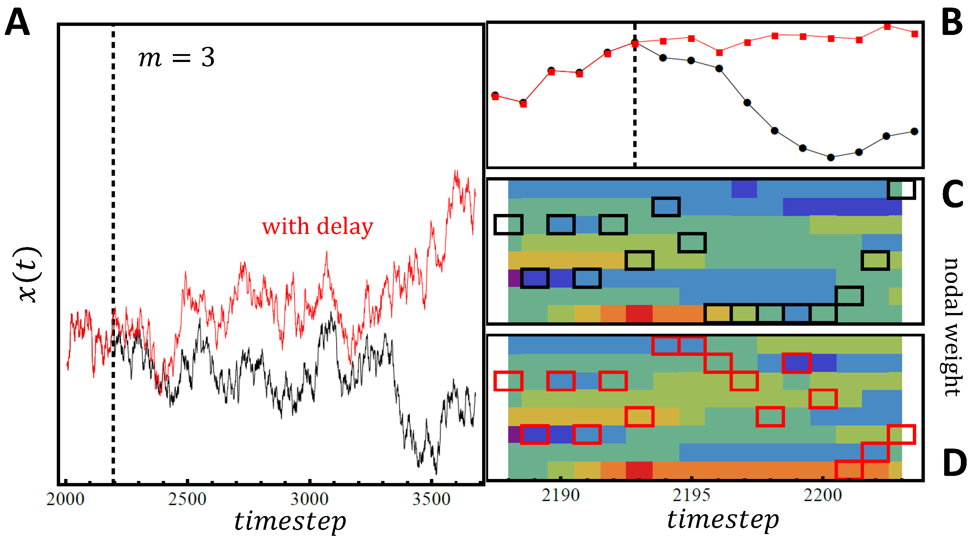
In the next section, we provide some more mathematical detail underlying these statements, but for now we focus on the numerical results from simulations of the DGCMC and GCMG. These are shown in Figure 5, Figure 6 and Figure 7. In Figure 5A we show the output (i.e., price ) of the GCMG and the DGCMG for with a small delay introduced at timestep . The population size and each agent has two strategies (). As in the basic MG, the GCMG and the DGCMG, the dimension of the strategy space is , where the memory is m[24,29]. Figure 5B shows a magnified version of Figure 5A focused around the time at which the delay is introduced . Figure 5C,D show the weights associated with the specific nodes for the GCMG (i.e., no delay) and DGCMG (i.e., with delay) respectively. A brief description will be given of the meaning of these weights in the next section, but they are discussed in detail in Ref. [25]. Although the delay introduced is small, it is interesting that the trajectories of the DGCMC (red) and GCMG (black) systems quickly diverge as a result (Figure 5A,B). This is likely because there are only 8 nodes in the de Bruijn graph for , hence the system can be easily disrupted from its Eulerian trail around it. While the GCMG is following a fixed-node behavior with persistence on a particular node (Figure 5C), by contrast the DGCMG (Figure 5D) quickly cycles out of it. Higher m values (not shown) imply a higher dimension of the strategy space, hence it might be guessed that the larger number of nodes will suppress the likelihood of the system following highly-correlated pathways in the de Bruijn graph. However this is not necessarily the case: we still find some unexpected extreme events generated by the system.
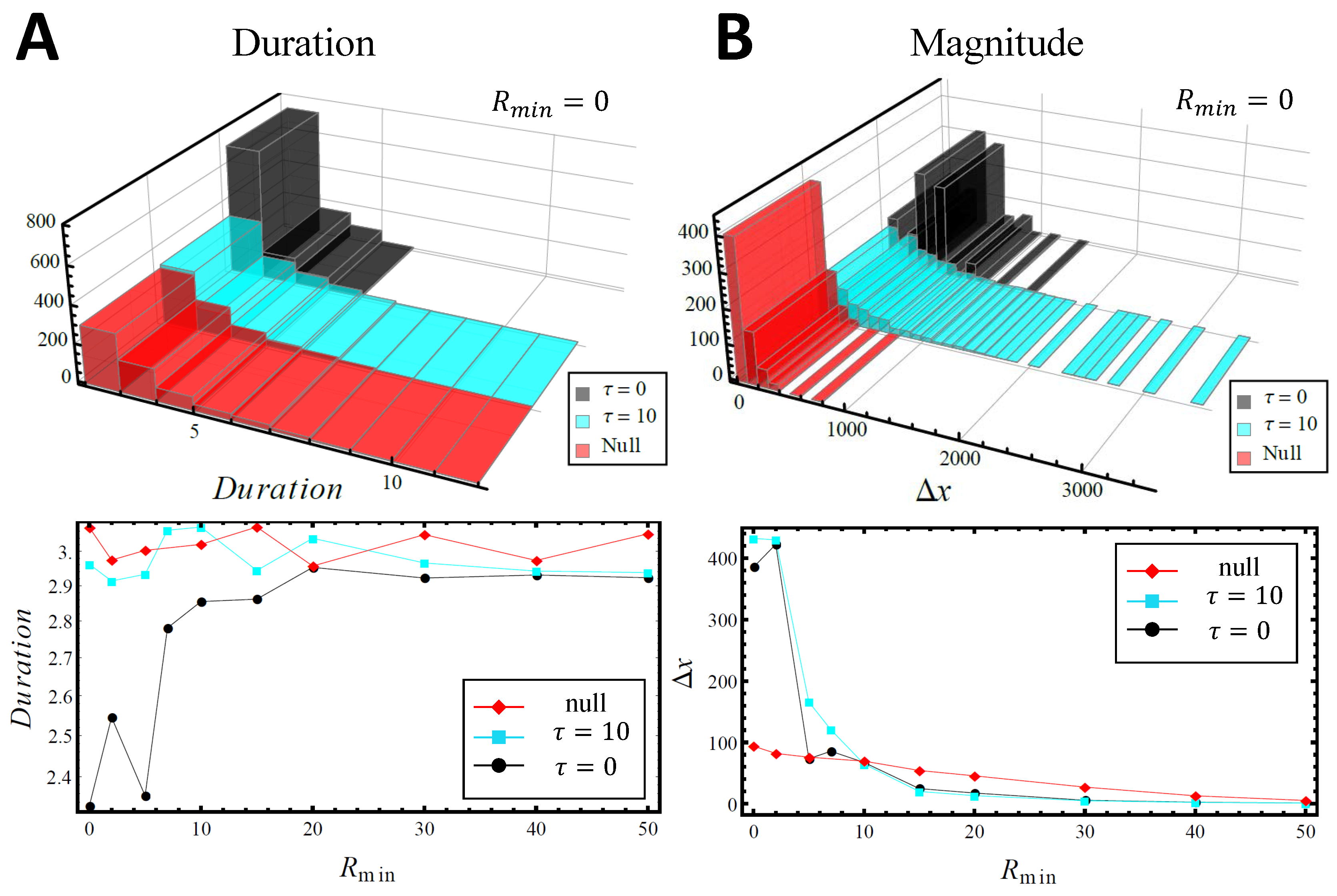
Figure 6 turns to look at the impact of the delay on the duration and magnitude (i.e., severity) of the extreme events generated by the the delay . Specifically, Figure 6 looks into single-node extreme events for three cases: GCMG, DGCMG and null-GCMG. The null-GCMG consists of an analogous set-up to the GCMG: however instead of using s strategies, agents use s coins to decide the action. Since the agents use coins, there is no pre-determined action for a particular piece of global information (i.e., a particular bit-string history length m). Instead, the coin-flip determines an equal probability for each option and . As in the GCMG, each strategy receives a score after each timestep according to its performance. Figure 6A shows our results for a single-node crash duration while Figure 6B shows the corresponding results for the magnitude. Both upper panels depict the distribution for these three models when the threshold for participation is zero over a period of timesteps (i.e., , noting that in principle can in general be set to be negative or positive). We find that although the delay tends to increase the duration of such extreme events, it is not notably different from the null version. However the magnitude shows that the DGCMG and the null-GCMG are indeed highly contrasting models showing a much larger magnitude for the DGCMG that compares, on average, to that of the GCMG. This can be explained with the fact that the null-GCMG is uncorrelated and hence the excess demand on average tends to zero. On the other hand the GCMG and DGCMG experience the crowding effect (see Section 5.1) and hence the resultant correlated excess demand contributes to a much greater extreme event magnitude. The lower panels show that as the confidence threshold for participation increases, the outcomes for the three models tend toward the same behavior for both duration and magnitude.
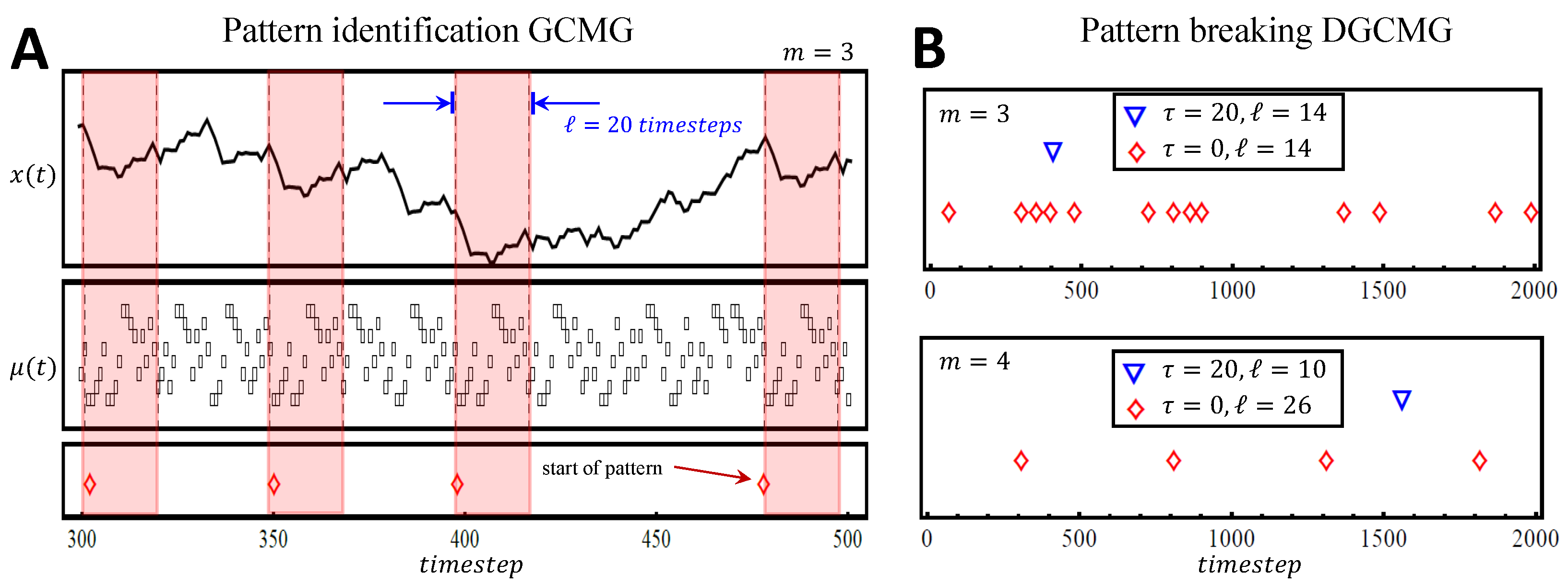
Another way to investigate the impact of latency (i.e., delays) is by looking at the pattern formation in the global information. As found in the MG, the global information frequently follows periodic patterns whose lengths agree with the quasi-deterministic Eulerian trail of period [24,29]. Figure 7 shows an example of this for the case of and where we explored latency values of , and 100. Figure 7A illustrates a pattern of time-length equal to appearing four times in an interval of 200 timesteps for the case of (Eulerian trail period is equal to 16 for ). The top panel shows the output change while the middle panel shows the global information with the shaded regions highlighting the pattern’s location. The bottom panel shows that, in a simplified way, the diamonds point to the start of the pattern. Figure 7B builds on this simplification to compare the pattern formation for the case when the latency is implemented. We find that the frequency as well as the length of the pattern is drastically reduced. For the top panel of Figure 7B illustrates that while a specific 14 step-length pattern is found 13 times over a period of 2000 game repetitions in the GCMG, it is only found once for DGCMG for the case of . Other values of latency are not found to contain this specific pattern for lengths larger than 10. For (Eulerian trail period equal to 32) a pattern of length 26 is found four times over a 2000 timestep interval, as shown in the bottom panel of Figure 7B. By contrast, the DGCMG does not show this pattern for the values explored. However a subset of length 10 of the original pattern is found only once for the case of . We attribute this pattern breaking to the systematic delay which breaks up the correspondence between the agents’ strategy scores and the global outcome. Developing a full theory of these effects and observations is currently an open question which we hope will be addressed in future work.
5. Results: Analytics
A full theory of the simulation results for both the DGCMG and the GCMG represents a fascinating open research challenge. Here we simply provide some elements of the analytics that we believe can be used as building blocks toward this goal.
5.1. Crowding
The following simple explanation of why extreme behaviors can arise more frequently and with bigger magnitude than for a system of independent stochastic components (like N coins), holds in principle for the MG, the GCMG and the DGCMG. We start with an observation about the strategy space, which then guides the argument. It turns out that the action output from two arbitrarily chosen strategies can sometimes be approximated as being either perfectly correlated, perfectly anti-correlated, or perfectly uncorrelated. While this is not typically the case for two arbitrary strategies in the full implementation of the game, it is a good approximation for the game run with a reduced strategy space. Most importantly, this reduced strategy space game produces essentially identical output to the full strategy space game, but it is much easier to analyze. Specifically, the Full Strategy Space FSS contains all possible permutations of the actions and for each history. As such there are strategies in this space. A dimensional hypercube shows all strategies from the FSS at its vertices. However one can choose a subset of strategies (i.e., Reduced Strategy Space RSS) such that any pair within this subset is either perfectly correlated, ant-correlated or uncorrelated. For example, any two agents using the same () strategy would take the same action irrespective of the sequence of previous outcomes and hence the dynamics of the game. Hence the two agents’ actions are perfectly correlated. By contrast, any two agents using the strategies and respectively, would take the opposite action irrespective of the sequence of previous outcomes. Hence the two agents’ actions are perfectly anti-correlated. Meanwhile, any two agents using the strategies and respectively, would take the opposite action for two of the four sets of previous outcomes, while they would take the same action for the remaining two. Hence the two agents’ actions are perfectly uncorrelated. Most importantly, running a given game simulation within the RSS reproduces the main features obtained using the FSS. The RSS has a smaller number of strategies than the FSS which has . In short, the RSS provides a minimal set of strategies which span the FSS and are hence representative of its full structure. It is this feature that helps us understand the size of the fluctuations to be expected. If we pair up these RSS strategies into their correlated and anti-correlated pairs, each of these pairs will be uncorrelated with each other. Given that a measure of the fluctuations in the output is given by the variance, we can therefore write the variance of the output as the sum of the variances for each correlated-anticorrelated strategy pair, i.e., the crowd and its anti-crowd. The average number of agents using strategy K therefore do the opposite of the average number using the anticorrelated strategy irrespective of the global outcome bit-string. Hence the effective group-size for each crowd-anticrowd pair is : this represents the net step-size d of the crowd-anticrowd pair in a random-walk contribution to the total variance. Hence, the net contribution by this crowd-anticrowd pair to the variance is given by
where for a random walk. Since all the strong correlations have been removed (i.e., anti-correlations), the separate crowd-anticrowd pairs execute random walks which are uncorrelated with respect to each other. Hence the total variance is given by the sum of the individual variances:
The competitive nature of the game means that no single strategy is a priori better than any other, and so the ordering of the strategies in terms of their scores will change continually and quickly. Hence we can relabel the strategies by their ranking in terms of numbers of points. To evaluate the above equation for , we just need to work out how many agents hold the strategy that is ranked the overall best at any moment. Hence we can simply sum up the number of agents who hold that strategy. The fact that there are a small number of strategies compared to the number of components (agents) means that there will be a similar number of agents holding each of the possible sets of s strategies. This means that the number holding the best strategy at any time, given by , will tend to scale like N. Since there is a threshold in the GCMG and DGCMG for playing, the number of agents who will play the anti-correlated strategy is essentially zero, since it will by definition have the lowest number of points (i.e., lowest ranking) and hence will likely be below the threshold. This means that the fluctuations will scale as , or rather that the standard deviation of will scale as N. By contrast for a system of N coins (i.e., N independent and hence uncorrelated agents), it is well known from the physics of random walks that the standard deviation of will scale as . Hence we have explained why the GCMG and DGCMG should show larger magnitude extreme behaviors than both the MG (where the number of agents playing the anti-correlated strategy can be significant) and a random null-model system comprising N independent coins.
5.2. GCMG Nodal Weighting Analysis
In the GCMG and DGCMG, the strategy score vector (with components ) is given by
where the vector contains the respective actions or for the global information at time t. Since a large fluctuation (i.e., extreme event) occurs when many agents take the same action, it will tend to occur when many agents hold the same strategy, i.e., N is much larger than the number of strategies and hence m is small. This is the regime in which the following discussion has validity.
Full details of the following discussion are given in Ref. [24] from which this material is adapted. The GCMG (and hence the DGCMG at times prior to the added delay) are both highly competitive games and hence tend to follow an anti-persistent path around the de Bruijn graph, with opposite consecutive transitions for visits to any given node. At each transition, since it either adds or removes a point to the scores according to the minority winning action, there is therefore an addition of an increment to the score vector . There are P orthogonal increment vectors since there is one for each node . If we choose the initial scores , this means that the strategy score vector can be expanded exactly in terms of these orthogonal components as follows:
where represents the ’nodal weight’ for global information node . It is these nodal weights that are shown and referred to in the earlier figures. The nodal weights all fluctuate near a net score of 0 because the strategy scores in the small m game are all highly mean-reverting. These nodal weights are very useful for building a fuller theory because they count the difference between the number of negative return transitions from node and the number of positive return transitions, in the time window . A high value of the absolute nodal weight implies that there is persistence in the transitions from that node and hence persistence in the excess demand—and hence the system can appear over consecutive timesteps to be moving in one direction or another, i.e., up or down, in a reasonably persistent way which is exactly what is required in order to have an episode of extreme behavior. In short, such extremes in the output behavior will occur when connected nodes become persistent. There are many possible forms for extreme behaviors based on the trajectories into which they become locked as a result of these nodal weights. The simplest that shows perfect nodal persistence is in which all successive changes are in the same direction (as in Figure 5C). We refer to this as a fixed-node crash or dip (or, if upwards, spike), and in general fixed-node extreme event. A slightly more complicated example can be understood by referring to the de Bruijn graph: the cycle which features four out of the five possible transitions yielding changes of the same sign. In other words, it is anti-persistent on node but is persistent on nodes . We refer to this as a cyclic-node crash or dip (or, if upwards, spike). Extreme changes can for example start as a fixed-node crash and then subsequently become a cyclic-node crash.
For the fixed-node crash, if the trajectory lands on any of the nodes with abnormally high nodal weights, there will likely be a large change in the system. For the GCMG (and DGCMG) at small m, whether a strategy is played is dictated by whether its score is above the threshold . The excess demand and volume defined earlier, can then be written approximately as
For a fixed node extreme event, we start by supposing that the persistence on node starts at time . To calculate the duration of the resulting large change, we expand the contributions into strategies with action at (), and those with action (). Suppose node was not visited during the previous T timesteps: Since and are orthogonal, the loss of score increment from time-step does not then affect on average. During the large change, at any later time , we hence have
The large change therefore ends at time when the right-hand side of Equation 7 changes sign. since decreases as the persistence time increases. This yields an expression for the persistence time or duration of the large change: . The calculation proceeds in the following way:
5.3. DGCMG Impact of Delays
In principle, a delay can be added into the above expressions and the resulting magnitude and durations calculated and compared for the GCMG and DGCMG as a function of . In this paper, however, we aim for the far more modest goal of simply stating in words the likely effect. One might think that since the delay removes the coordination between the strategy score vector and the node at which the system sits in the de Bruijn graph, it is essentially equivalent to adding more noise to the system and hence makes it more likely to be closer to the null model of coin tosses. This would suggest that the duration and magnitude of extreme changes would be smaller in the DGCMG than in the GCMG. However this argument is clearly over-simplistic since there are many examples in the simulations of the DGCMG where large events do occur – perhaps through some stochastic resonance effect. We will leave this for future study.
6. Results: Real World Data
While it is too early to be able to match up patterns from the simulation, analytics, and actual real-world extreme events, we provide here a glimpse of what arises in the actual sub-second market system. The electronic financial exchanges are not only the largest and fastest societal networks, they are the most data-rich. On a scale of microseconds, one-body and two-body interactions (quotes and trades, respectively) are automatically recorded. Given the lack of possible real-time human activity on the sub-second scale (Figure 3), it is not too surprising that the system output is often machine-like in that it appears with short-term, deterministic behaviors which are far from a coin-toss random walk [24]. Such a heavily deterministic system can drive can hence generate extreme sub-second behaviors as a result of driving the system in definite directions. Latency can also naturally occur, because of bottlenecks in communication etc.
Figure 8 provides an example of how small delays can have large unintended consequences in terms of system-level output. We stress that the underlying machinery is not as simple as the DGCMG, but it is interesting to note that delays in this real system do indeed feed back to drive the crowd of algorithmic decision-makers in the same direction, just as Figure 4 might suggest. The example of extreme sub-second system behavior that is shown in Figure 8A, arose recently from an otherwise typical stock (Suncor) on an otherwise typical day, and within a time window of 500 milliseconds (i.e., s). Figure 8B shows how the delays accumulated like shockwaves, and hence effectively provided delayed global information to the population of agents (i.e., trading algorithms) which then produced a crowd-like response which drove the price up in an unexpected and unusual way. Figure 8C provides further simulation output from the GCMG and DGCMG to show how it is not too difficult to obtain similar results from the simulations with delay. It also however warns that the question of when delays will enhance or suppress potential extreme events and behaviors, needs to be explored in a more systematic way: specifically, large change labelled 1 is apparently suppressed by the delay while large change 2 seems unchanged by it.
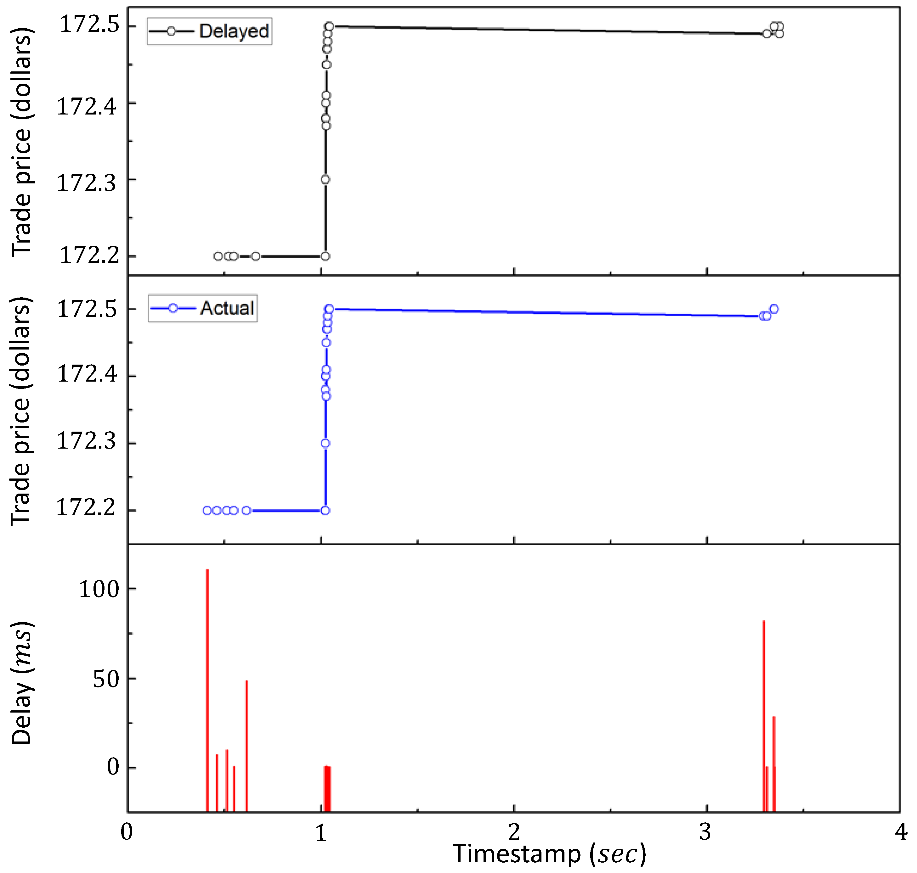
Figure 9, and the examples from Figure 1, show more generally that an extraordinarily wide variety of extreme behaviors can occur on the sub-second scale in this all-electronic decentralized system on an otherwise ordinary day. Figure 1 focused on dips and spikes, while Figure 9 shows that the system output can suddenly rise to a much larger value over a few consecutive steps, and then flatten out with no subsequent activity for a relatively long time (i.e., no participating agents). The system corresponds to the trade price of the stock AAP trading on the NYSE exchange. The top panel shows the delayed-time price which is openly available. The middle panel shows these same trades at the actual times that they occurred: these true-time data require a significant fee to access and hence most agents only have access to the delayed data. The bottom panel shows the time difference between each trade event’s actual time of occurrence and the delayed time at which it was reported. Though we cannot conclude that the large changes showed in Figure 1 or Figure 9 are caused by delays, these curious observations motivate further investigation of both the GCMG and the DGCMG.
We also stress that although a full theory and classification of such extreme behaviors awaits further analysis, the fact that they emerge from a decentralized all-electronic system should make them of interest to a far broader community than just the finance industry.
7. Conclusions
Many future electronic systems upon which society depends, will likely follow the same path that financial trading has taken in terms of evolving into an effective all-electronic ecology in which a centralized real-time controller is impractical. Even if a centralized real-time controller could be created, it would likely contradict laws forbidding monopolies and data-sharing. Instead, the individual components belonging to different companies will likely openly compete with each other based on only limited global information [1,2]. They will also likely have limited processing power and algorithmic complexity because of finite battery capacity and the need for speed. Even if most societal cyber-physical systems are not yet at that level, this is indeed currently the case with the financial exchanges in both the U.S. and Europe. Motivated by this, this paper has compared two highly non-trivial generalizations of the Minority Game: the Grand Canonical Minority Game (GCMG) and the Delayed Grand Canonical Minority Game (DGCMG) which adds delays in global information arrival. We have also tried to inspire future analytical work focused toward a full theory of these systems.
Acknowledgments
N.F.J. is very grateful to NANEX, and specifically Eric Hunsader, for freely sharing financial datasets that NANEX assembled, and to Paul Jefferies for earlier collaborations on the formalism. This material is based upon work supported by the U.S. National Science Foundation (NSF) under grant 1522693 and the Air Force Office of Scientific Research under award number FA9550-16-1-0247. Any opinions, finding, and conclusions or recommendations expressed in this material are those of the authors and do not necessarily reflect the views of the NSF or the United States Air Force.
Author Contributions
N.F.J. and P.M.H. conceived and designed the study; P.D.M. and M.Z. performed the calculations; P.D.M., M.Z., Z.C., D.D.J.R. and N.F.J. analyzed the results; N.F.J. and P.D.M. wrote the paper. All authors revised and approved the manuscript.
Conflicts of Interest
The authors declare no conflict of interest.
References
- Edward, A.L. The Past, Present and Future of Cyber-Physical Systems: A Focus on Models. Sensors 2015, 15, 4837–4869. [Google Scholar]
- Loiseau, P.; Schwartz, G.A.; Musacchio, J.; Amin, S.; Sastry, S.S. Incentive mechanisms for internet congestion management. IEEE/ACM Trans. Netw. 2014, 22, 647–661. [Google Scholar] [CrossRef]
- Lee, E.A. Computing Foundations and Practice for Cyber-Physical Systems: A Preliminary Report; Technical Report UCB/EECS-2007-72; University of California: Berkeley, CA, USA, 2007. [Google Scholar]
- Rajkumar, R. A cyber-physical future. Proc. IEEE 2012, 100, 1309–1312. [Google Scholar] [CrossRef]
- Li, X.Y.; Wang, Y.Y.; Zhou, X.S.; Liang, D.F. Approach for cyber-physical system simulation modeling. J. Syst. Simul. 2014, 3, 631. [Google Scholar]
- Liu, Y.; Peng, Y.; Wang, B.; Yao, S.; Liu, Z. Review on Cyber-physical Systems. IEEE/CAA J. Autom. Sin. 2017, 4, 27–40. [Google Scholar]
- Konstantakopoulos, I.C.; Ratliff, L.; Jin, M.; Spanos, C.; Sastry, S.S. Smart Building Energy Efficiency via Social Game: A Robust Utility Learning Framework for Closing the Loop. In Proceedings of the 1st International Workshop on Science of Smart City Operations and Platforms Engineering (SCOPE) (ACM/IEEE CPSWeek), Vienna, Austria, 12–14 April 2016. [Google Scholar]
- Calderone, D.; Mazumdar, E.; Ratliff, L.; Sastry, S.S. Understanding the Impact of Parking on Urban Mobility via Routing Games on Queue Flow Networks. In Proceedings of the IEEE 55th Conference on Decision and Control (CDC), Las Vegas, NV, USA, 12–14 December 2016. [Google Scholar]
- Zebulum, R.S.; Pacheco, M.A.C.; Vellasco, M.M. Evolutionary Electronics; CRC Press: Boca Raton, FL, USA, 2002. [Google Scholar]
- Conway, B. Wall Street’s Need For Trading Speed: The Nanosecond Age. Available online: http://blogs.wsj.com/marketbeat/2011/06/14/wall-streets-need-for-trading-speed-the-nanosecond-age/ (accessed on 1 October 2017).
- Pappalardo, J. New Transatlantic Cable Built to Shave 5 Milliseconds off Stock Trades. Available online: http://www.popularmechanics.com/technology/engineering/infrastructure/a-transatlantic-cableto-shave-5-milliseconds-off-stock-trades (accessed on 1 October 2017).
- Lewis, M. Flash Boys: A Wall Street Revolt; W.W. Norton & Company: New York, NY, USA, 2014. [Google Scholar]
- McCoy, K. IEX Exchange Readies for Mainstream Debut. 18 August 2016. Available online: http://tabbforum.com/news/iex-exchange-readies-for-mainstream-debut?utm_campaign=d19dc21bc0-UA-12160392-1&utm_medium=email&utm_source=TabbFORUM%20Alerts&utm_term=0_29f4b8f8f1-d19dc21bc0-278278873 (accessed on 18 August 2016).
- Johnson, N.F.; Zhao, G.; Hunsader, E.; Qi, H.; Johnson, N.; Meng, J.; Tivnan, B. Abrupt rise of new machine ecology beyond human response time. Sci. Rep. 2013, 3, 2627. [Google Scholar] [CrossRef] [PubMed]
- Manrique, P.D.; Zheng, M.; Restrepo, D.D.J.; Hui, P.M.; Johnson, N.F. Impact of delayed information in sub-second complex systems. Results Phys. 2017, 7, 3024–3030. [Google Scholar] [CrossRef]
- Johnson, N.F. Simply Complexity; Oneworld: Oxford, UK, 2009. [Google Scholar]
- U.S. Commodity Futures Trading Commission. Findings Regarding the Market Events of 6 May 2010. Available online: http://www.sec.gov/news/studies/2010/marketevents-report.pdf (accessed on 1 October 2017).
- Krafcik, J. Say Hello to Waymo: What’s Next for Google’s Self-Driving Car Project. Available online: https://medium.com/waymo/say-hello-to-waymo-whats-next-for-google-s-self-driving-car-project-b854578b24ee.mrpkjhhm9 (accessed on 22 February 2016).
- Uber to Introduce Self-Driving Cars within Weeks. Available online: http://www.bbc.com/news/technology-37117831. (accessed on 18 August 2016).
- Kramer, D. White House Encourages Adoption of Drones. Phys. Today 2016. Available online: http://scitation.aip.org/content/aip/magazine/physicstoday/news/10.1063/PT.5.1080?utm_source=Physics%20Today&utm_medium=email&utm_campaign=7427978_The%20week%20in%20Physics%208\T1\textendash12%20August&dm_i=1Y69,4F7GQ,E1O09U,GA27B,1 (accessed on 9 August 2016).
- Vespignani, A. Predicting the behavior of techno-social systems. Science 2009, 325, 425–428. [Google Scholar] [CrossRef] [PubMed]
- Eagleman, D. How does the timing of neural signals map onto the timing of perception? In Space and Time in Perception and Action; Nijhawan, R., Ed.; Cambridge University Press: Cambridge, UK, 2010. [Google Scholar]
- Johnson, N.F.; Hart, M.; Hui, P.M.; Zheng, D. Trader dynamics in a model market. Int. J. Theor. Appl. Financ. 2000, 3, 443. [Google Scholar] [CrossRef]
- Johnson, N.F.; Jefferies, P.; Hui, P.M. Financial Market Complexity; Jefferies, P., Phil, D., Eds.; Oxford University Press: Oxford, UK, 2003; Chapter 4. [Google Scholar]
- Jefferies, P.; Lamper, D.; Johnson, N.F. Anatomy of extreme events in a complex adaptive system. Phys. A Stat. Mech. Appl. 2003, 318, 592–600. [Google Scholar] [CrossRef]
- Johnson, N.F.; Hui, P.M. Crowd-anticrowd theory of dynamical behavior in competitive, multi-agent autonomous systems and networks. J. Comput. Intell. Electron. Syst. 2015, 3, 256–277. [Google Scholar] [CrossRef]
- Moro, E. The Minority Game: An Introductory Guide. Available online: http://arxiv.org/pdf/cond-mat/0402651.pdf (accessed on 1 October 2017).
- Challet, D.; Chessa, A.; Marsili, A.; Chang, Y.C. From Minority Games to Real Markets. Quant. Financ. 2001, 1, 168–176. [Google Scholar] [CrossRef]
- Jefferies, P.; Hart, M.; Johnson, N.F. Deterministic dynamics in the minority game. Phys. Rev. E 2002, 65, 016105. [Google Scholar] [CrossRef] [PubMed]
- Choe, S.C.; Johnson, N.F.; Hui, P.M. Error-driven global transition in a competitive population on a network. Phys. Rev. E 2004, 70, 055101. [Google Scholar] [CrossRef] [PubMed]
- Zhao, L.; Yang, G.; Wang, W.; Chen, Y.; Huang, J.; Ohashi, H.; Stanley, H.E. Herd behavior in a complex adaptive system. Proc. Natl. Acad. Sci. USA 2011, 108, 15058. [Google Scholar] [CrossRef] [PubMed]
- Liang, Y.; An, K.N.; Yang, G.; Huang, J.P. Contrarian behavior in a complex adaptive system. Phys. Rev. E 2013, 87, 012809. [Google Scholar] [CrossRef] [PubMed]
- Helbing, D. Dynamic Decision Behavior and Optimal Guidance Through Information Services: Models and Experiments. In Human Behaviour and Traffic Networks; Schreckenberg, M., Selten, R., Eds.; Springer: Berlin/Heidelberg, Germany, 2004; p. 47. [Google Scholar]
- Cartlidge, J.; Szostek, C.; De Luca, M.; Cliff, D. Too fast, too furious. In Proceedings of the 4th International Conference on Agents & Artificial Intelligence, Vilamoura, Portugal, 6–8 February 2012. [Google Scholar]
- Johnson, N.F. To slow or not? Challenges in subsecond networks. Science 2017, 355, 801–802. [Google Scholar] [CrossRef] [PubMed]
- Johnson, N.F.; Tivnan, B. Mechanistic origin of dragon-kings in a population of competing agents. Eur. Phys. J. Spec. Top. 2012, 205, 65–78. [Google Scholar] [CrossRef]
Figure 1.
Subsecond tsunamis from a real-world decentralized, all-electronic system. The data comes from the U.S. network of market exchanges. (A) an example of an extreme spike in the price of a particular stock. The points are discrete since each corresponds to a specific event (i.e., a new trade). This is consistent with our decision to focus on discrete-time models in this paper. The number of sequential up ticks is 31, and the price change is +2.75. The duration is 25 ms (i.e., 0.025 s). The percentage price change upwards is (i.e., spike size is 0.26 expressed as a fraction). The size of the dots in price chart are proportional to volume of trade; (B) an example of an extreme dip in the price of a particular stock. The number of sequential down ticks is 20, and the change in output (i.e., price change) is −0.22. The duration is 25 ms (i.e., 0.025 s). The percentage price change downwards is (i.e., dip size is 0.14 expressed as a fraction).

Figure 2.
Size and duration for the ultrafast tsunamis that we observed in the 5-year period of data. There is no well-defined relationship between their size and duration. The fact that their size and duration are not trivially linked helps confirm their surprising nature.
Figure 2.
Size and duration for the ultrafast tsunamis that we observed in the 5-year period of data. There is no well-defined relationship between their size and duration. The fact that their size and duration are not trivially linked helps confirm their surprising nature.

Figure 3.
Schematic shows the typical timescales for human action (i.e., intervention), electronic hardware operations, and for running software including trading algorithms. The limits of electronic hardware coincide with the lower limit set by the phonon scattering time. Switching processes in typical electronic circuits determine the operating time of software algorithms. As a result, the relevant regulatory bodies face a daunting task of how to ensure system safety and (in a market setting) fairness to all participants in terms of when they receive relevant information. Moreover, regulatory bodies need to provide this reassurance without relying on any real-time human intervention during moments of potential subsecond-scale instability.

Figure 4.
(A) The Delayed Grand Canonical Minority Game (DGCMG) that we study in this paper, is a modification of the Grand Canonical Minority Game which was introduced in Ref. [23]. Specifically it has an added temporal delay in the feedback of global information to the agents, as compared to the GCMG. The N components (called here ’agents’) each have s strategies (labeled by ) that are chosen randomly from the strategy space in order to mimic heterogeneity in the component population. The global information, delayed by timesteps, , and the scores of the strategies are used by each agent to decide whether to take the action or the action . For all timesteps , the delay for both the GCMG and the DGCMC. At any given timestep in both cases, only agents who have a strategy with a score greater than a threshold value will take part in the game. To mimic a highly competitive environment, we consider the winning action (i.e., global outcome) to correspond to the action taken by the minority. At time , we change from zero to a positive real number in the DGCMG introducing a temporal delay (i.e., latency). For , all timesteps in the DGCMG have this same delay value , while for the GCMG ; (B) Transitions of the global information can be shown conveniently on a de Bruijn graph, with each possible transition shown by an arrow. It is shown for (upper panel) and (lower panel). Each node carries a binary bit-string denoting the most recent m global outcomes, and the equivalent integer representation shown in red parenthesis, e.g., for the nodal bit-string
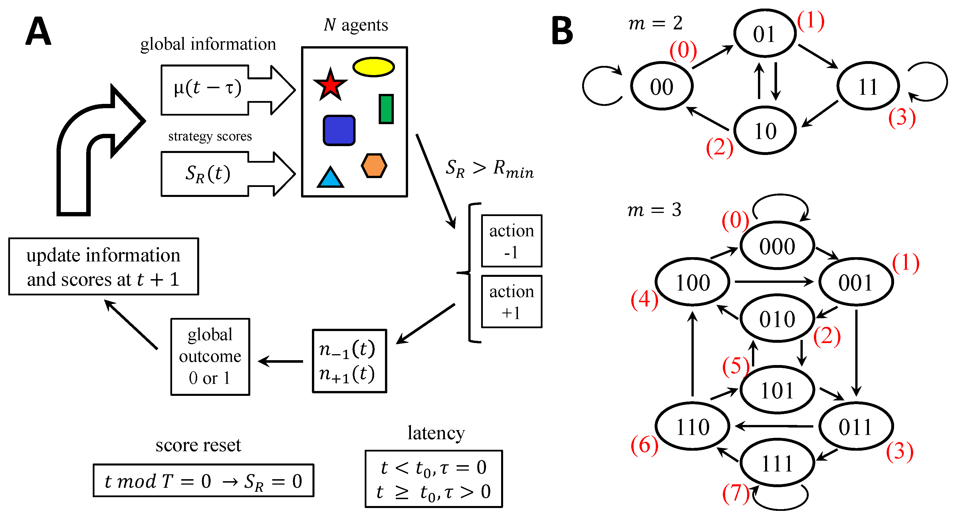
Figure 5.
(A) System output (e.g., price) for the GCMG (black line—no delay) and the DGCMG (red line—delay introduced at timestep ). The population of components (i.e., agents) has size : each inputs the system-wide reported information (see Figure 2) and can output an action; (B) Panel A magnified around , the time of the delay implementation; (C) Dynamics of GCMG shown in terms of the nodal weights (see main text); (D) Corresponding dynamics of DGCMG. In (C,D), there are nodal weights at each timestep, shown on the y-axis, corresponding to the possible nodes in the de Bruijn graph. The highest weight is red while lowest is purple.

Figure 6.
(A) Simulation results for fixed-node extreme events in a system of agents with strategies per agent and . The DGCMG corresponds to a delay of timesteps as compared to the GCMG where by definition. The null model (see text) is unchanged by a delay, since it involves memoryless coins for strategies. Upper panel shows the distribution of durations for a given threshold , while lower panel shows the mean duration as a function of ; (B) Analogous to A but for magnitude rather than duration. The magnitude is defined as the price difference before and after the event.

Figure 7.
(A) Dynamical patterns in the GCMG for the case of . Top panel shows the price (), middle panel shows the global information () and the bottom panel uses diamonds to signal the start of a dynamical pattern. The 20 timestep length patterns are highlighted by the red shaded region; (B) Pattern breaking effect of latency for (top) and (bottom). Symbols represent pattern appearances of a given length ℓ, for a delay .

Figure 8.
(A) The network of networks of U.S. electronic exchanges produces multiple examples of sub-second extreme behavior. In this example, the data-points show trades (i.e., prices of trade events) for Suncor stock within a 500 millisecond (i.e., s) time interval. Each color corresponds to a different electronic exchange network within the larger network of U.S. exchange networks. They are physically interconnected by communications channels. Data was kindly provided by NANEX; (B) Orange dots show the delay (vertical axis) between the time at which a particular trade event was reported system-wide and the time at which it actually occurred in a particular network exchange (which is shown on the horizontal axis). These delays predate the intentional 350 microsecond delay added in 2016 [13], however the fact that they show such strong temporal correlations demonstrates the possible effect of such an intentional (and hence highly temporally correlated) delay. The parallel diagonal lines show the shockwaves of successive trades eventually getting reported system-wide. The fact that these waves of system-wide reporting occur a few milliseconds ahead of significant dynamical features in panel A, is likely due to each reporting shockwave driving the networks’ trading algorithms (i.e., agents) to produce a sudden change in aggregate supply and demand, which the appears a few milliseconds later as a new dynamical feature in panel A; (C) DGCMG system output (red line) showing the price over time following a small delay introduced at . Black line shows same system but with no delay, i.e., GCMG. Window 2 shows a future extreme behavior akin to panel A that still occurs with the delay, while window 1 shows a future extreme behavior that effectively disappears when the delay is added.
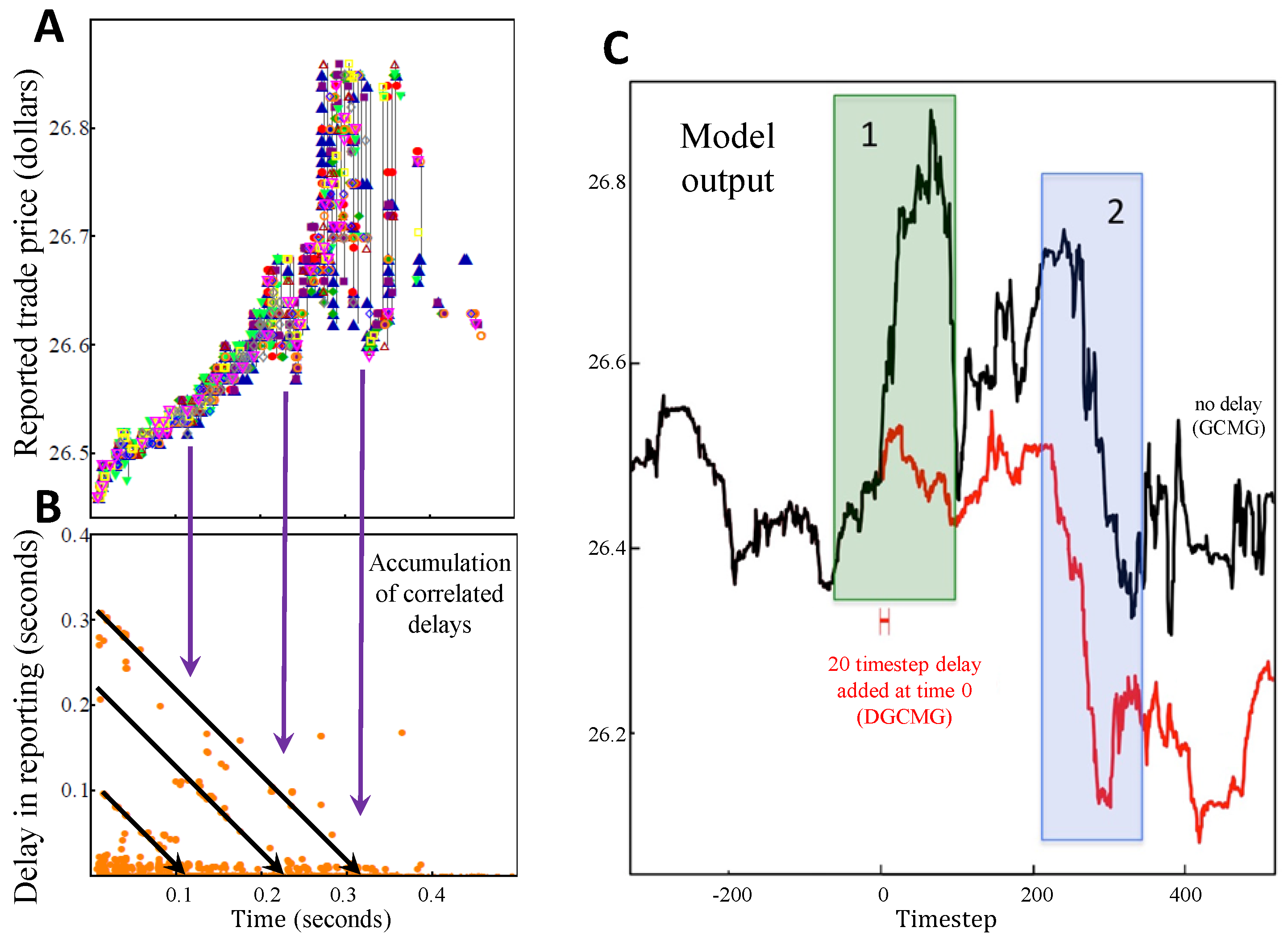
Figure 9.
Example of a stock’s trades on the NYSE exchange within a 4 s interval on an otherwise ordinary day. The top panel shows the price of each trade as a function of the delayed reporting time, which is the time information that is publicly available. Middle panel shows the actual time of the trade (i.e., without delay). Bottom panel shows the latency between the actual time and the delayed time.

© 2017 by the authors. Licensee MDPI, Basel, Switzerland. This article is an open access article distributed under the terms and conditions of the Creative Commons Attribution (CC BY) license (http://creativecommons.org/licenses/by/4.0/).
Share and Cite
MDPI and ACS Style
Manrique, P.D.; Zheng, M.; Cao, Z.; Johnson Restrepo, D.D.; Hui, P.M.; Johnson, N.F. Subsecond Tsunamis and Delays in Decentralized Electronic Systems. Electronics 2017, 6, 80. https://doi.org/10.3390/electronics6040080
AMA Style
Manrique PD, Zheng M, Cao Z, Johnson Restrepo DD, Hui PM, Johnson NF. Subsecond Tsunamis and Delays in Decentralized Electronic Systems. Electronics. 2017; 6(4):80. https://doi.org/10.3390/electronics6040080
Chicago/Turabian StyleManrique, Pedro D., Minzhang Zheng, Zhenfeng Cao, David Dylan Johnson Restrepo, Pak Ming Hui, and Neil F. Johnson. 2017. "Subsecond Tsunamis and Delays in Decentralized Electronic Systems" Electronics 6, no. 4: 80. https://doi.org/10.3390/electronics6040080
Note that from the first issue of 2016, this journal uses article numbers instead of page numbers. See further details here.