DoA and DoD Estimation and Hybrid Beamforming for Radar-Aided mmWave MIMO Vehicular Communication Systems


1
School of Electronic and Information, Shanghai Dianji University, Shanghai 201306, China
2
State Key Laboratory of Millimeter Waves, School of Information Science and Engineering, Southeast University, Nanjing 210096, China
3
Science and Technology on Electromagnetic Scattering Laboratory, Shanghai 200438, China
4
Xi’an branch of China Academy of Space Technology, Xi’an 710100, China
*
Author to whom correspondence should be addressed.
†
These authors contributed equally to this work.
Electronics 2018, 7(3), 40; https://doi.org/10.3390/electronics7030040
Submission received: 29 January 2018
/
Revised: 4 March 2018
/
Accepted: 15 March 2018
/
Published: 18 March 2018
Abstract
:In millimeter wave (mmWave) communications, the feature of relatively large signal absorption and directional transmission render new challenges for wireless communications and signal processing. To further improve the performance of mmWave communications, a novel radar-aided mmWave communication (RAMC) approach is proposed, which can be used in vehicular communications. There are two parts in the proposed RAMC system, including the radar subsystem and the mmWave communication subsystem. In the radar subsystem, the bistatic co-prime multi-input and multi-output (MIMO) arrays are considered. With the radar antenna arrays, both the directions of departure (DoD) and the directions of arrival (DoA) are estimated. Additionally, the compressed sensing (CS)-based method is proposed to obtain the target positions. Using the estimated angle and position information, the channel estimation and feedback link of the mmWave communication subsystem can be eliminated. Moreover, a hybrid beamforming algorithm is proposed in the mmWave communication subsystem, which can overcome the shortage of the analog-only beamforming. Simulation results show that the better estimation performance can be achieved by the bistatic co-prime MIMO arrays than that by the traditional uniform linear arrays (ULA), and with the radar aided, the mmWave communication subsystem can reduce the beam search time, and the cell discovery time is improved significantly.
1. Introduction
Millimeter wave (mmWave) communications have been receiving tremendous interest by academia, industry and government as an option to realize the 5G cellular systems. The frequency band for the mmWave communications is from 30 GHz to 300 GHz. Therefore, it can offer higher-bandwidth channels, and meet the requirements for the remarkable growth of wireless data traffic. However, the propagation characteristics of mmWave system are different to those of the traditional sub-6 GHz system. Additionally, the heavy rainfall also brings about 7 dB/km attenuation for the mmWave propagation at 28 GHz [1,2]. To overcome the high path and penetration losses, the multiple-input and multiple-out (MIMO) with antenna beamforming plays a pivotal role in establishing and maintaining a robust communication link [3,4,5,6,7,8]. Additionally, since the wavelength of mmWave communications is smaller than that of the sub-6 GHz wave, the large antenna arrays can be implemented in smaller size at both the transmitter and receiver. For example, IEEE 802.11ad with 32 elements has already been deployed commercially.
With the beamforming technology, the directional communication can be realized with improved link capacity. There are mainly two types of beamforming, i.e., digital beamforming and analog beamforming [6,9]. Digital beamforming is usually designed to work in baseband and provides a higher spatial degree of freedom and better performance for multi-user simultaneous transmission. Analog beamforming is usually designed to work in radio frequency (RF) chain and is effective for generating a narrow directional beamformer from a large number of antennas. Therefore, a hybrid beamforming is proposed and offers a tradeoff between the performance and the complexity [10,11,12]. Based on different applications, hybrid beamforming can be categorized into fixed weight beamforming and adaptive weight beamforming. In the fixed weight beamforming, constant antenna weights are applied to the array elements in the analog or digital domain to steer the main beam. In the adaptive beamforming, the RF radiation pattern can be adapted according to the time-varying direction-of-arrival (DoA) and direction-of-departure (DoD), where the efficient signal processing algorithms can be utilized to continuously resolve the desired signal and interfering signal.
However, in the traditional mmWave communications, the following issues have not yet been tackled efficiently. In the adaptive beam and sector selection, the training vectors are sent first, then the beam and sector with the best communication condition are chosen. However, since the position of the receiver is unknown, the existing methods including both the exhaustive search and the hierarchic search algorithms must search the whole beam space and sectors to figure out the exact beam and sector in which the receiver lies. However, the computational complexity is very high. Since the distance from the moving vehicles to the base station is unknown, it is difficult for the inter-cell handover, e.g., cell discovery and user discovery. It is a common challenge to mitigate the interference for the cell-edge users in existing multi-cell multi-user systems. Especially for the fast moving vehicles with frequent inter-cell handover, such as the high speed train (HST), much more overhead is needed to process the inter-cell handover, which will lead to low data rate, e.g., less than M bps for the GSM-R and around 2 M bps for the new-developed broadband wireless communication for HST in Japan, Taiwan and Europe. Therefore, in this paper, a radar-aided mmWave communication (RAMC) system is proposed to tackle the aforementioned issues [13,14,15,16,17]. As shown in Figure 1, there are two parts in the RAMC system:
- The MIMO radar subsystem is only involved in the transmitter, the positions and velocities of vehicles are estimated. With the assistance of the radar, it is much easier to detect and track the moving vehicles. Moreover, radar can also be used to distinguish the shape of different vehicles in civil transportations in the city, e.g., identifying the bus from cars and trucks.
- In the mmWave MIMO communication subsystem, based on the parameters including positions and velocities obtained from the MIMO radar system, the efficiency as well as the performance of channel estimation, sector and beam selection, hybrid beamforming, cell discover and inter-cell handover can all be improved.
The remainder of this paper is organized as follows. The bistatic co-prime MIMO arrays and mmWave MIMO communication system are given in Section 2, and in this section, the CS-based method is proposed for the DoD and DoA estimation. Section 3 describes the hybrid beamforming in the mmWave communication subsystem. The simulation results are given in Section 4. Finally, Section 5 concludes the paper.
Notations: denotes the expectation operation. denotes an identity matrix. denotes the complex Gaussian distribution with the mean being and the variance matrix being . , , , ⊗, , and denote the norm, the norm, Frobenius norms, the Kronecker product, the vectorization of a matrix, the matrix transpose and the Hermitian transpose, respectively.
2. System Descriptions
In the proposed RAMC system, antennas of the radar subsystem and mmWave communication subsystem are seperated. The bistatic co-prime arrays in the radar subsystem are adopted in both transmitter and receiver [18,19,20,21,22], and the massive MIMO antennas are adopted in the mmWave communication subsystem. We can describe the two parts separately in detail.
2.1. System Model for Radar Subsystem
The bistatic co-prime arrays in the radar subsystem are adopted in both transmitter and receiver [16,18,19,20,21,22,23]. The number of antennas in transmitter and receiver are () and (), respectively. Two sub-arrays are adopted in transmitter, and the relative antenna positions are denoted as () in the first sub-array, and () in the second sub-array, where d denotes the fundamental antenna spacing. Similarly, in receiver, the relative antenna positions are denoted as () in the first sub-array, and () in the second sub-array. In the first transmitter sub-array, the signal in the -th antenna is denoted as . In the second transmitter sub-array, the signal of the -th antenna is denoted as . With K far-field targets, the received signal in the -th antenna of the first receiver sub-array can be formulated as
where denotes the scattering coefficient of the k-th target, denotes a diagonal matrix with the diagonal entries from , denotes the additive white Gaussian noise (AWGN), and
Similarly, the received signals in the -th antenna of the second RX sub-array can be expressed as
where
After the matched filters corresponding to the transmitted signals, we can obtain the following vectors of the received signals
Therefore, the signals after the matched filter can be rewritten into a matrix form as
where
Then, with the received signal , we can obtain a vector form as
where , and , and . , and .
Compressed Sensing-Based DoA and DoD Estimation Method
With the received signal , we can define the following dictionary matrix
where Z denotes the number of discretized DoA or DoD, , and the z-th column of is also denoted as . Therefore, the original problem of DoA and DoD estimation will become the sparse reconstruction problem
where is adopted to control the estimation accuracy and can be usually set as , and denotes the sparse vector, the non-zero entries are the target scattering coefficients, and the positions of the non-zero entries indicate the DoA and DoD [16,17,18,24,25].
To reconstruct the sparse vector , the orthogonal matching pursuit (OMP) method [24,26,27] can be adopted. Algorithm 1 shows the details of the OMP algorithm to estimate the target scattering coefficients, DoD and DoA. The DoD and DoA can be obtained from the index set of the non-zero entries.
| Algorithm 1 OMP algorithm for DoA and DoD estimation |
|
2.2. System Model for mmWave Communication Subsystem
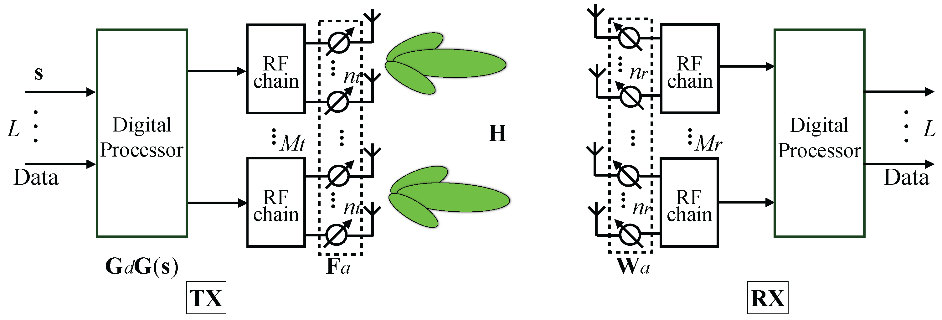
In this paper, we consider a single-user mmWave communication subsystem and mainly focus on the downlink transmission shown in Figure 2. The transmitter (TX) with antennas communicates data streams to the RX with antennas. The antenna array at the TX is connected to the analog beamformer that is implemented by phase shifters, and the analog beamformer at the RX is equipped with RF chains.
Since the mmWave channels have sparse scattering, it is inappropriate to assume the entries of to be i.i.d. Gaussian random variables, the ray-tracing representations can be used to model the mmWave channel [28]. Assuming that there are K scattering clusters and each one contributes to a single propagation path between the TX and RX. The channel can be expressed as
where is the fading gain of the path, and are the antenna array response vectors at the TX and RX, respectively. Assuming that the antenna arrays are installed in the horizontal direction, we denote and as the departure and arrival directions of the kth path, where and are the physical azimuth angles of departure and arrival. With assuming the variation of the channel is only caused by the path gains and this assumption is based on the mmWave channel measurements in [29], we can derive that the clusters’ central angles belong to large-scale fading and the path gains belong to small-scale fading. For notational convenience, (12) can be rewritten in a compact form as
where denotes the path gain matrix, and represent the transmit and receive antenna element gain at the corresponding angels of departure and arrival.
Assuming the uniform linear arrays (ULAs) are used at the TX, the array response vector can be written as
and can be obtained in the similar way.
Based on the above description, the RX received signal can be given by
where is the Gaussian noise vector.
At the TX side, assuming the transmite data symbols are precoded by the nonlinear digital procoder and mapped into data streams, . The digital beamformer , followed by an analog beamformer . The discrete-time transmitted signal is given by
For notational convenience, (16) can be rewritten in a compact form as
where denotes the hybrid digital/analog beamforming matrix, and can be written as
where represents the modulus and phase of the mth analog phase shifter, and the entries are of constant modulus.
3. The Hybrid Beamforming
In this paper, we focus on a single-user downlink transmission, where the large antenna array is driven by a limited number of transmit/receive chains. However, the same algorithms can be directly applied to the uplink system, where the channel is replaced by the uplink channel, and the analog beamformers, of the transmitter and receiver are switched.
In this section, we address the problem of designing the hybrid beamformers [30,31,32,33,34]. In the design of hybrid beamforming, the power is usually maximized, so the direction of beam can be designed to the users. Therefore, in our paper, we consider the design of weight matrix to maximize the received power.Since the analog beamformer at the RX is more simple than the transmitter, we first discuss the receiver side, and then discuss the hybird beamformer design for the transmitter.
In order to simplify the system model, there is no baseband combiner in the RX and the received signal is processed by the analog phase shifters and the digital processor directly, which result in
3.1. Analog Beamformer Design for the Receiver
For simplicity, assuming the elements in the transmitted signal ), and the average power of (19) can be represented as
substituting (13) into (20) we have
where ,
In particular, the RX analog beamforming matrix takes the form
where denotes the modulus and phase of the analog phase shifter in the antenna subarray.
According to (21) and (22), we can maximize the receive power by solving the following optimization problem
where is the sub-matrix of , which from row to the row. By solving (23), we can obtain the expression of and finally get the analog beamforming matrix .
If we relax the constraint of (23) as , it is obvious that the is the eigenvector corresponding to the biggest eigenvalue of , i.e. . Consider the constrain, we can adjust the phase of the antenna sub-array as
where “ / ” represents division of the elements, “” represents the modulus of each element.
Since can be represented by
then, using (24) to adjust will result in . To avoid this situation, we can calculate the eignvalue and the corresponding eignvectors for arbitrary , and we can obtain the expression of as follows
where .
The Hybrid Beamformer Design of the Transmitter
The hybrid beamformer design is similar with the receiver side, here we seek to maximize the average transmitted power of the K azimuth angles. The average transmitting power can be written as
where denotes the variance of the symbol stream. Since maximizing the average transmitting power is equivalent to solve the following optimization problem
where , . However, directly solving (28) is intractable, so we can first reference the solution of (23) to obtain , and then give the solution of g.
Let represent the sub-matrix of A that from row to row . By solving the eignvalue of , and the corresponding eignvector , we have
where .
According to (29), we can obtain the analog beamformer , then the digital beamforming matrix can be obtained by solving the following optimization problem
It is obvious that (30) is a convex optimization problem, we can obtain the optimize results by the KKT (Karush-Kuhn-Tucker) condition. The Lagrange function can be written as
the KKT conditions of (30) are: (a) ; (b) ; (c) ; (d) , where represents the Lagrange multiplier. The expression of the optimal that satisfy the above conditions can be written as
Since the hybrid beamforming algorithms of the transmitter and receiver both belong to long-term beamforming algorithm, the matrix and F has no relationship with the path gain , and has only been affected by the DoA, DoD and the transmit power.
4. Simulation Results
In this section, the simulation results are given, and the simulation parameters are set as follows: the carrier frequency of the transmitted signals is GHz, the speed of light is m/s, the wavelength is cm, the fundamental antenna spacing , the parameters of transmitting antennas are and , the parameters of receiving antennas are and , and the number of targets is .
In Figure 3, the OMP method is used to estimate the target positions, where the 5 targets randomly distribute in the area and . In the OMP algorithm, the numbers of discretized DoD and DoA are both 100, so the size of the dictionary matrix is , and the length of received signals is 133. The length of the vector is and only 5 entries are non-zeros, so the DoD and DoA estimation problem is a sparse reconstruction problem, and the proposed OMP method can be used. This is shown in Figure 3, where the signal-to-noise ratio (SNR) is 20 dB. The DoD and DoA can be exactly estimated in the scenario with the uncorrelated targets, but when the two targets are close to each other and the targets are correlated, the estimation performance also degraded.
In Figure 4, we compare the DoD and DoA estimation performance with different numbers of targets, where the root mean square error (RMSE) is defined as
where denote the estimated DoD and DoA in the n-th Monte Carlo simulation, respectively, and denotes the total number of the Monte Carlo simulations. As shown in Figure 4, the estimation performance is improved by improving the SNR of received signals. With less targets, the estimation performance can approach the CRLB as shown in this figure. Since the target correlation is improved with more targets, the estimation performance is also degraded by adding more targets.
In Figure 5, the DoD and DoA estimation performance of co-prime is compared with that of ULA, where the numbers of transmitting and receiving antennas are the same in both co-prime and ULA. The SNR of received signal is 20 dB. As shown in Figure 5, when the CS-based method is used to estimate the DoD and DoA, the better performance can be achieved by the bistatic co-prime MIMO arrays than that by the ULA. Therefore, the bistatic co-prime MIMO arrays outperform the transitional ULA. Figure 6 also gives the angle bias with different values of SNR.
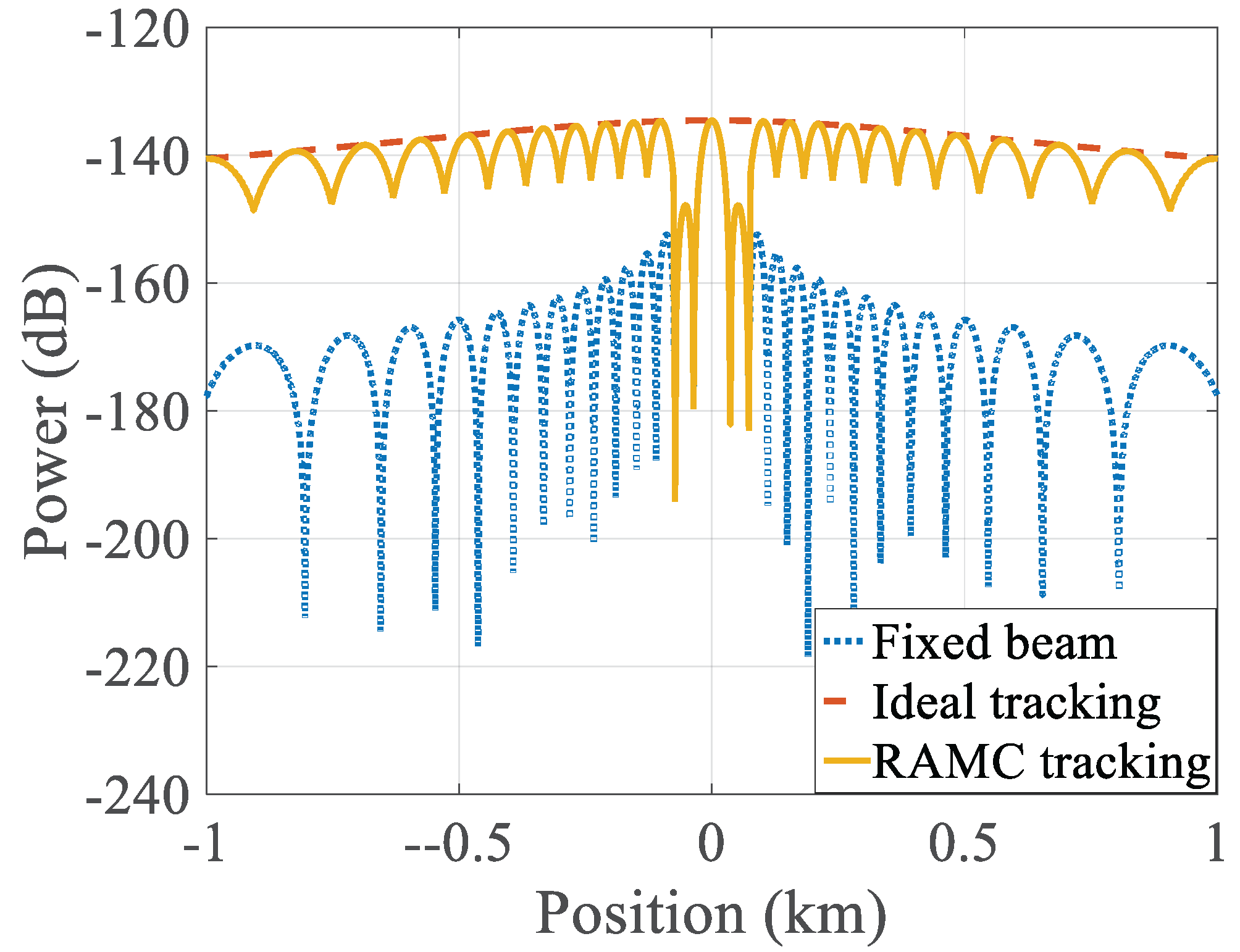
In Figure 7, we compare the received power of the RAMC system with the ideal tracking and the existing fixed beam system (no tracking). In the RAMC system, the beams are adaptively updated in every of angle. It is observed that the received power of the RAMC system can be significantly improved and closer to that of ideal tracking than the fixed beam system.
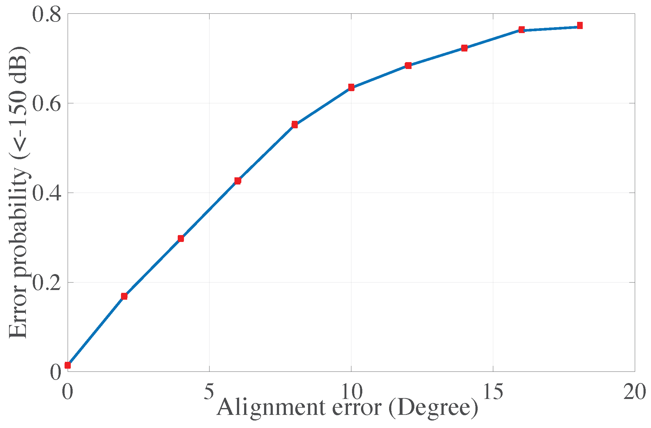
Once the beam is perfectly aligned to the vehicles, the received power will be the largest and meanwhile the power efficiency is the highest. However, in practice, it usually has some errors for the beam alignment. Figure 8 shows the probability that the received power is smaller than dB, where the largest received power is dB according to Figure 7. Therefore, in the RAMC system, MIMO radar plays an important role, where the accuracy in estimating the user position by radar determines the accuracy of beam alignment and power efficiency.
For the beam and sector selections, the position obtained by radar can help to decrease the time to search the beam that the receiver lies in. Compared with the existing algorithms including the exhaustive beam search algorithm and hierarchic beam search algorithm, the candidate beamspace for the search is substantially shrunk with the radar’s position information. As shown in Figure 9, the beam search time of both the exhaustive and hierarchical algorithms are compared with that of the proposed RAMC. In this comparison, for the initial search of the first beam, the MIMO radar system has no prior knowledge about the position of vehicle, so the search time is the same with the exhaustive search, meaning that the two curves are overlapped. However, in Figure 10, we assume that there are 50 base stations and the interval of two base stations is 2 km. After the radar detects the vehicles, it keeps the tracking of the vehicles. When the radar system starts to track the moving vehicles, the beam search time can be significantly decreased compared to both the exhaustive and hierarchical search algorithms.
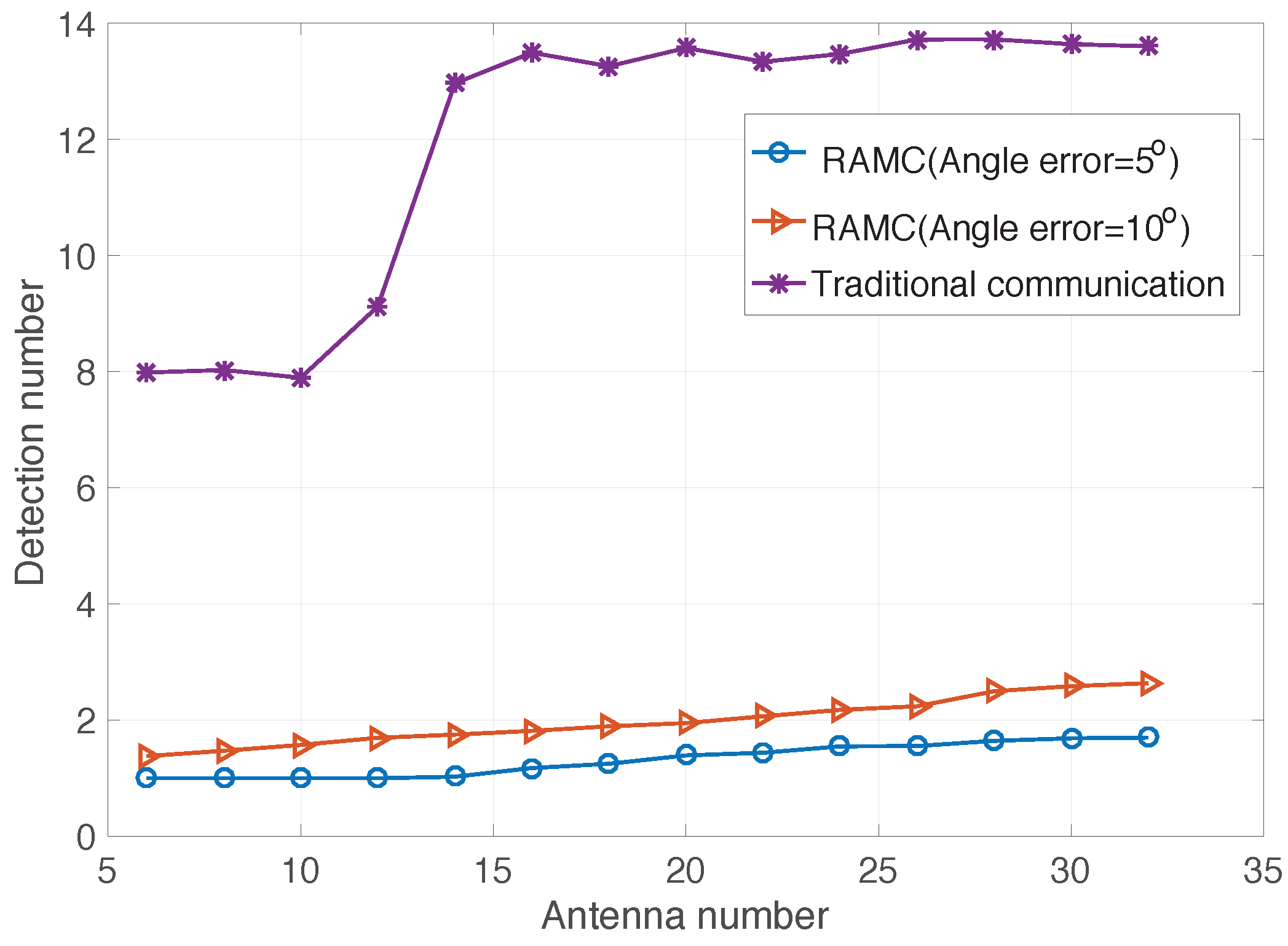
The cell discovery time in the RAMC system is compared with that of the traditional mmWave communication in Figure 11. With increasing number of antennas, the main lobe of beam pattern is becoming narrower. Therefore, more search slots are needed to find the new user. However, compared with the traditional method, since the RAMC system can detect and track the new added user, much less slots are needed in the proposed system to find the new user. Additionally, in the radar system, there are errors in the angle estimation for the new user, as shown in this figure. We compare the search slots with the maximum errors of the estimated angle being and . As shown in this figure, the accurate estimation can increase the efficiency to find the new user, so the estimation performance of the MIMO radar system must be guaranteed in the proposed system. The angle accuracy can be achieved by equipping more antennas to the MIMO radar system.
5. Conclusions
In the proposed RAMC system, the overhead for channel estimation, sector and beam selection, cell discovery and inter-cell handover can be greatly reduced. The adaptive hybrid beamforming can be implemented more easily. Note that the proposed RAMC system is different from the traditional joint radar and communication system, where the same waveform is used for both the communication and target estimation in the joint radar and communication system. In the proposed RAMC system, different waveforms are adopted for target estimation and communication. Additionally, we can set the radar and the mmWave working in different frequency bands, so that the interference between radar and communication systems can be also eliminated. Moreover, the radar and communication system can be independently optimized to further improve the performance. Future works will focus on the parameter estimation in the moving coprime arrays and the system optimization.
Acknowledgments
This work was supported in part by the National Natural Science Foundation of China (Grant No. 61601281, 61471117, 61501298, 61603239), and the Open Program of State Key Laboratory of Millimeter Waves (Southeast University, Z201804).
Author Contributions
Zhimin Chen and Peng Chen conceived and designed the experiments; Zhenxin Cao performed the experiments; Zhenxin Cao and Xinyi He analyzed the data; Yi Jin and Jingchao Li contributed reagents/materials/analysis tools; Zhimin Chen wrote the paper.
Conflicts of Interest
The authors declare no conflict of interest.
References
- Rangan, S.; Rappaport, T.S.; Erkip, E. Millimeter wave cellular wireless networks: potentials and challenges. Proc. IEEE 2014, 102, 366–385. [Google Scholar] [CrossRef]
- Heath, R.W.; González-Prelcic, N.; Rangan, S.; Roh, W.; Sayeed, A.M. An Overview of Signal Processing Techniques for Millimeter Wave MIMO Systems. IEEE J. Sel. Top. Signal Process. 2016, 10, 436–453. [Google Scholar] [CrossRef]
- MacCartney, G.R.; Rappaport, T.S. 73 GHz millimeter wave propagation measurements for outdoor urban mobile and backhaul communications in New York City. In Proceedings of the 2014 IEEE International Conference on Communications (ICC), Sydney, Australia, 10–14 June 2014; pp. 4862–4867. [Google Scholar]
- Akoum, S.; Ayach, O.E.; Heath, R.W. Coverage and capacity in mmWave cellular systems. In Proceedings of the 2012 Conference Record of the Forty Sixth Asilomar Conference on Signals, Systems and Computers (ASILOMAR), Pacific Grove, CA, USA, 4–7 November 2012; pp. 688–692. [Google Scholar]
- Singh, H.; Oh, J.; Kweon, C.; Qin, X.; Shao, H.R.; Ngo, C. A 60 GHz wireless network for enabling uncompressed video communication. IEEE Commun. Mag. 2008, 46, 71–78. [Google Scholar] [CrossRef]
- Alkhateeb, A.; Leus, G.; Heath, R.W. Limited Feedback Hybrid Precoding for Multi-User Millimeter Wave Systems. IEEE Trans. Wirel. Commun. 2015, 14, 6481–6494. [Google Scholar] [CrossRef]
- Wei, L.; Hu, R.Q.; Qian, Y.; Wu, G. Key elements to enable millimeter wave communications for 5G wireless systems. IEEE Wirel. Commun. Mag. 2014, 21, 136–143. [Google Scholar]
- Roh, W.; Seol, J.Y.; Park, J.; Lee, B.; Lee, J.; Kim, Y.; Cho, J.; Cheun, K.; Aryanfar, F. Millimeter-wave beamforming as an enabling technology for 5G cellular communications: Theoretical feasibility and prototype results. IEEE Commun. Mag. 2014, 52, 106–113. [Google Scholar] [CrossRef]
- Liang, L.; Xu, W.; Dong, X. Low-Complexity Hybrid Precoding in Massive Multiuser MIMO Systems. IEEE Wirel. Commun. Lett. 2014, 3, 653–656. [Google Scholar] [CrossRef]
- Rappaport, T.S.; MacCartney, G.R.; Samimi, M.K.; Sun, S. Wideband Millimeter-Wave Propagation Measurements and Channel Models for Future Wireless Communication System Design. IEEE Trans. Commun. 2015, 63, 3029–3056. [Google Scholar] [CrossRef]
- Alkhateeb, A.; Mo, J.; Gonzalez-Prelcic, N.; Heath, R.W. MIMO Precoding and Combining Solutions for Millimeter-Wave Systems. IEEE Commun. Mag. 2014, 52, 122–131. [Google Scholar] [CrossRef]
- Park, M.; Cordeiro, C.; Perahia, E.; Yang, L.L. Millimeter-wave multi-Gigabit WLAN: Challenges and feasibility. In Proceedings of the 2008 IEEE 19th International Symposium on Personal, Indoor and Mobile Radio Communications, Cannes, France, 15–18 September 2008; pp. 1–5. [Google Scholar]
- Hassanien, A.; Vorobyov, S.A. Transmit energy focusing for DOA estimation in MIMO radar with colocated antennas. IEEE Trans. Signal Process. 2011, 59, 2669–2682. [Google Scholar] [CrossRef]
- Amiri, R.; Behnia, F.; Zamani, H. Asymptotically efficient target localization from bistatic range measurements in distributed MIMO radars. IEEE Signal Process. Lett. 2017, 24, 299–303. [Google Scholar] [CrossRef]
- González-Prelcic, N.; Méndez-Rial, R.; Heath, R.W. Radar aided beam alignment in MmWave V2I communications supporting antenna diversity. In Proceedings of the 2016 Information Theory and Applications Workshop (ITA), La Jolla, CA, USA, 31 January–5 February 2016; pp. 1–7. [Google Scholar]
- Chen, P.; Zheng, L.; Wang, X.; Li, H.; Wu, L. Moving target detection using colocated MIMO radar on multiple distributed moving platforms. IEEE Trans. Signal Process. 2017, 65, 4670–4683. [Google Scholar] [CrossRef]
- Chen, P.; Zhan, P.; Wu, L. Clutter estimation based on compressed sensing in bistatic MIMO radar. In Proceedings of the 2017 International Conference on Communication, Control, Computing and Electronics Engineering (ICCCCEE), Khartoum, Sudan, 16–18 January 2017; pp. 1–6. [Google Scholar]
- Yang, Y.; Blum, R. MIMO radar waveform design based on mutual information and minimum mean-square error estimation. IEEE Trans. Aerosp. Electron. Syst. 2007, 43, 330–343. [Google Scholar] [CrossRef]
- Jiang, H.; Qi, H.; Yao, S. Direction finding of multiple targets using coprime array in MIMO radar. IEICE Commun. Express 2016, 6, 115–119. [Google Scholar] [CrossRef]
- Li, J.; Jiang, D.; Zhang, X. DOA estimation based on combined Uunitary ESPRIT for coprime MIMO radar. IEEE Commun. Lett. 2017, 21, 96–99. [Google Scholar] [CrossRef]
- Jia, Y.; Zhong, X.; Guo, Y.; Huo, W. DOA and DOD estimation based on bistatic MIMO radar with co-prime array. In Proceedings of the 2017 IEEE Radar Conference (RadarConf), Seattle, WA, USA, 8–12 May 2017; pp. 394–397. [Google Scholar]
- BouDaher, E.; Jia, Y.; Ahmad, F.; Amin, M.G. Multi-frequency co-prime arrays for high-resolution direction-of-arrival estimation. IEEE Trans. Signal Process. 2015, 63, 3797–3808. [Google Scholar] [CrossRef]
- Zheng, L.; Wang, X. Super-Resolution Delay-Doppler Estimation for OFDM Passive Radar. IEEE Trans. Signal Process. 2017, 65, 2197–2210. [Google Scholar] [CrossRef]
- Chen, P.; Qi, C.; Wu, L. Antenna placement optimisation for compressed sensing-based distributed MIMO radar. IET Radar Sonar Navig. 2017, 11, 285–293. [Google Scholar] [CrossRef]
- Chen, P.; Wu, L.; Qi, C. Waveform optimization for target scattering coefficients estimation under detection and peak-to-average power ratio constraints in cognitive radar. Circuits Syst. Signal Process. 2016, 35, 163–184. [Google Scholar] [CrossRef]
- Tropp, J.A.; Gilbert, A.C. Signal recovery from random measurements via orthogonal matching pursuit. IEEE Trans. Inf. Theory 2007, 53, 4655–4666. [Google Scholar] [CrossRef]
- Petropulu, A.P.; Poor, H.V. Measurement matrix design for compressive sensing—Based MIMO radar. IEEE Trans. Signal Process. 2011, 59, 5338–5352. [Google Scholar]
- Akdeniz, M.R.; Liu, Y.S. Millimeter wave channel modeling and cellular capacity evaluation. IEEE J. Sel. Areas Commun. 2014, 32, 1164–1179. [Google Scholar] [CrossRef]
- Alkhateeb, A.; Omar El Ayach, G.; Robert, W.; Heath, J. Channel Estimation and Hybrid Precoding for Millimeter Wave Cellular Systems. IEEE Trans. Signal Process. 2014, 8, 831–846. [Google Scholar] [CrossRef]
- Chen, Z.; Wu, L.; Chen, P. Efficient modulation and demodulation methods for multi-carrier communication. IET Commun. 2016, 10, 567–576. [Google Scholar] [CrossRef]
- Ayach, O.E.; Rajagopal, S.; Abu-Surra, S.; Pi, Z.; Heath, R.W. Spatially Sparse Precoding in Millimeter Wave MIMO Systems. IEEE Trans. Commun. 2014, 13, 1499–1513. [Google Scholar] [CrossRef]
- Han, S.; Chih-Lin, I.; Xu, Z.; Rowell, C. Large-scale antenna systems with hybrid analog and digital beamforming for millimeter wave 5G. IEEE Commun. Mag. 2015, 53, 186–194. [Google Scholar] [CrossRef]
- Mirza, J.; Ali, B.; Naqvi, S.S.; Saleem, S. Hybrid Precoding via Successive Refinement for Millimeter Wave MIMO Communication Systems. IEEE Commun. Lett. 2017, 21, 991–994. [Google Scholar] [CrossRef]
- Venugopal, K.; Alkhateeb, A.; Prelcic, N.G.; Heath, R.W. Channel Estimation for Hybrid Architecture Based Wideband Millimeter Wave Systems. IEEE J. Sel. Areas Commun. 2017, 35, 1996–2009. [Google Scholar] [CrossRef]
Figure 1.
Block diagram of the radar aided mmWave communication system.
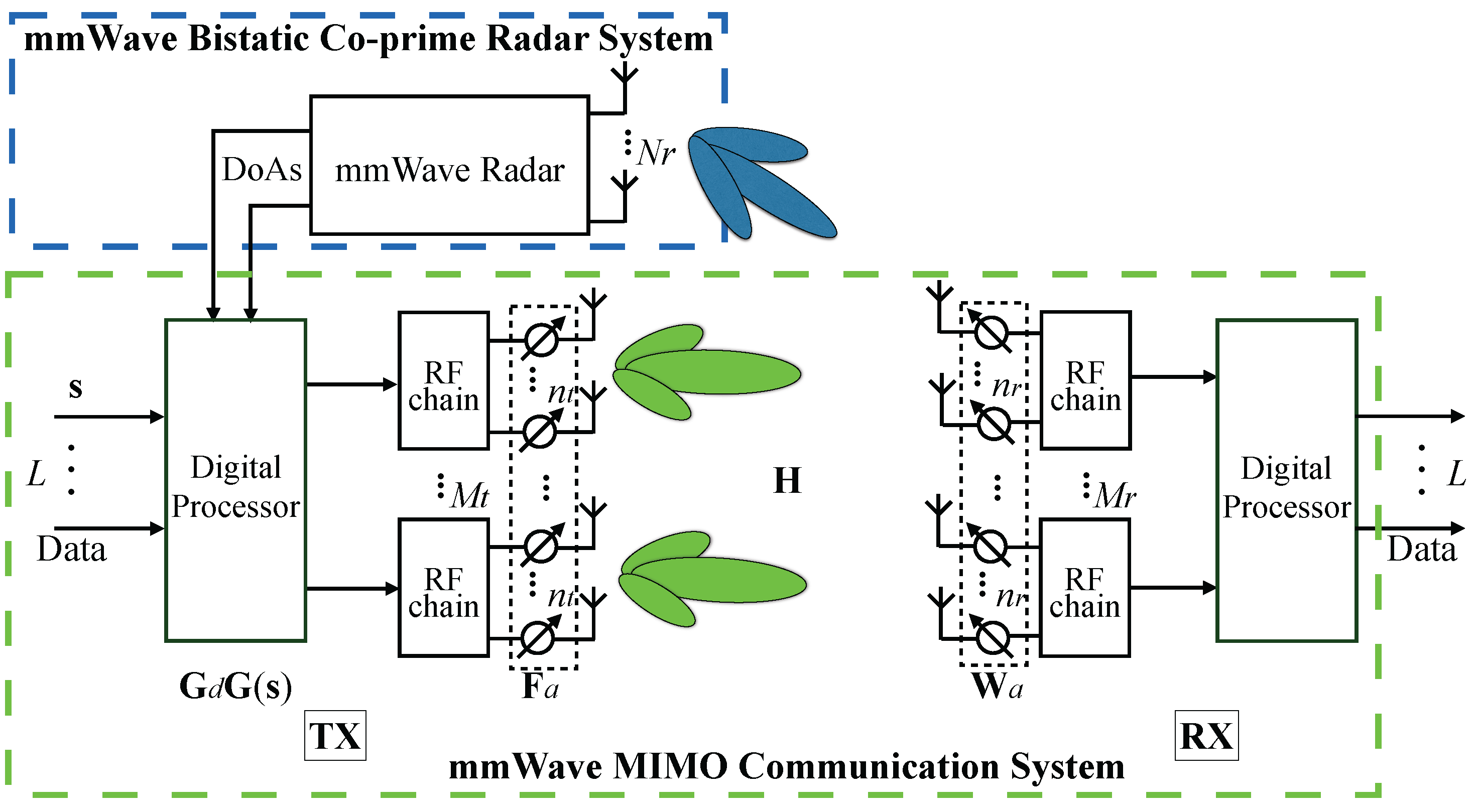
Figure 2.
The diagram of hybrid beamforming in the mmWave communication subsystem.

Figure 3.
The estimated target positions.
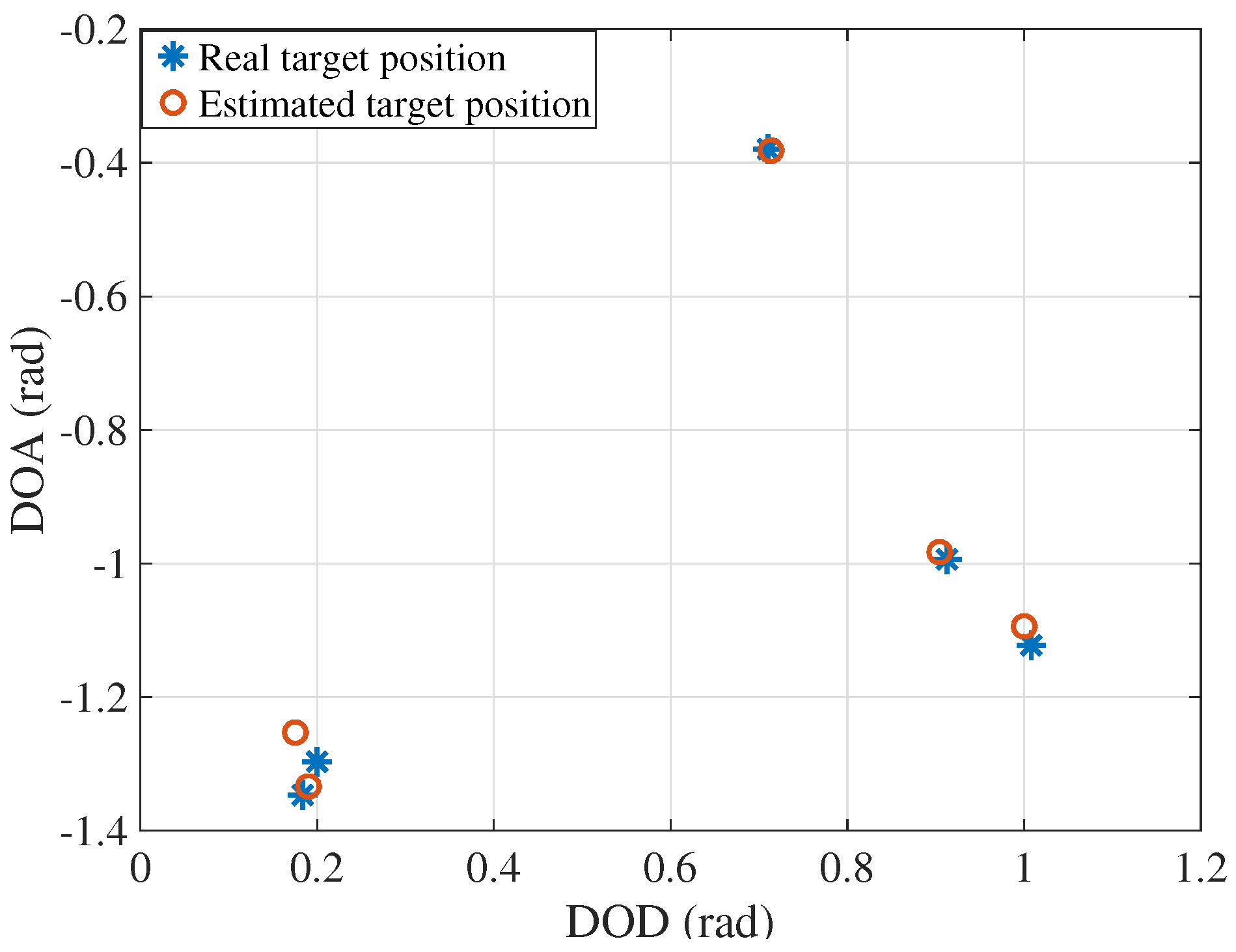
Figure 4.
The estimation performance with different numbers of targets.
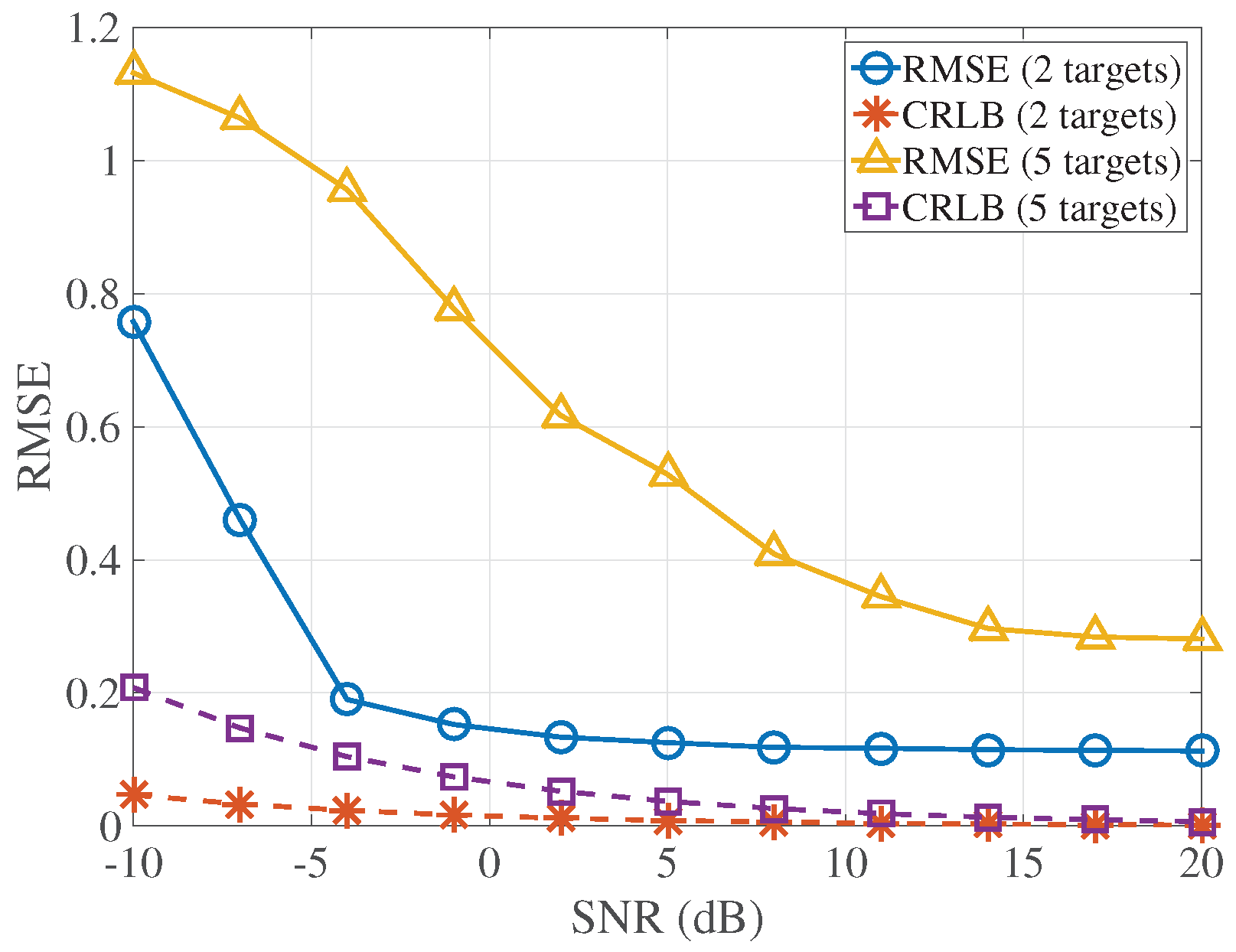
Figure 5.
The estimation performance compared with ULA.
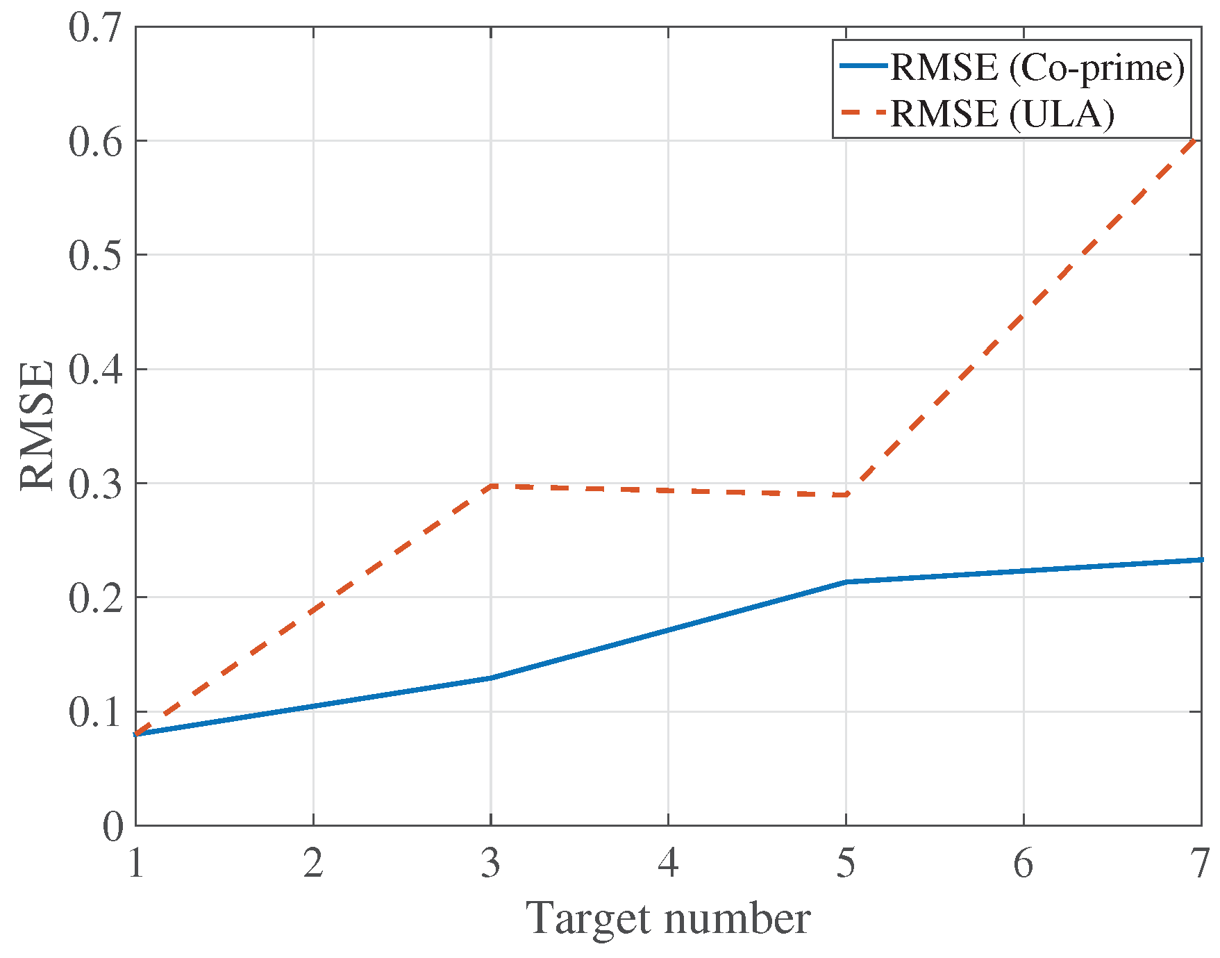
Figure 6.
The DoA and DoD estimation performance.
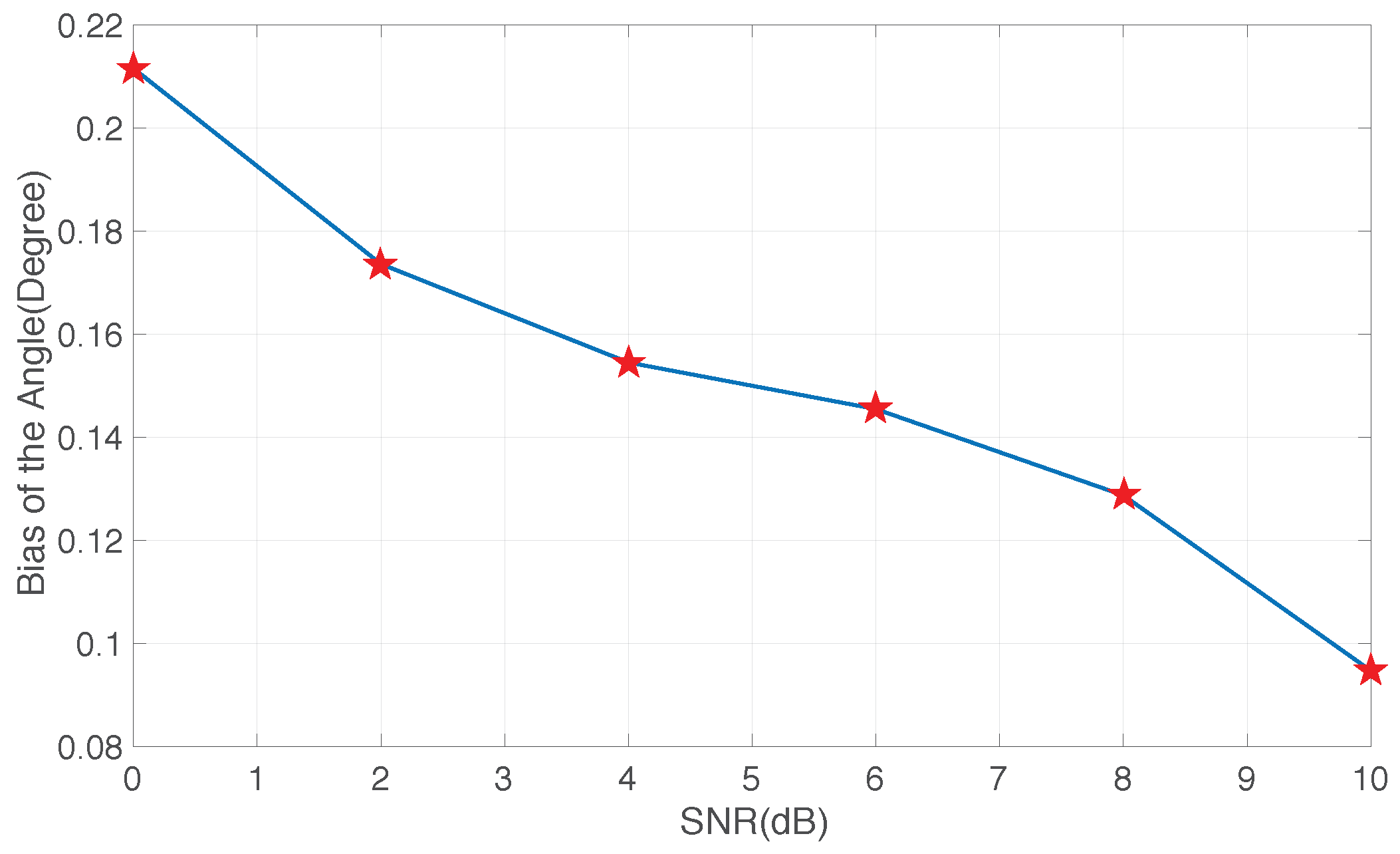
Figure 7.
Comparisons of the received power of RAMC with ideal tracking and fixed beam.

Figure 8.
The relationship between the estimated angle error and received power.

Figure 9.
Beam search time in MIMO radar system by the first base station.
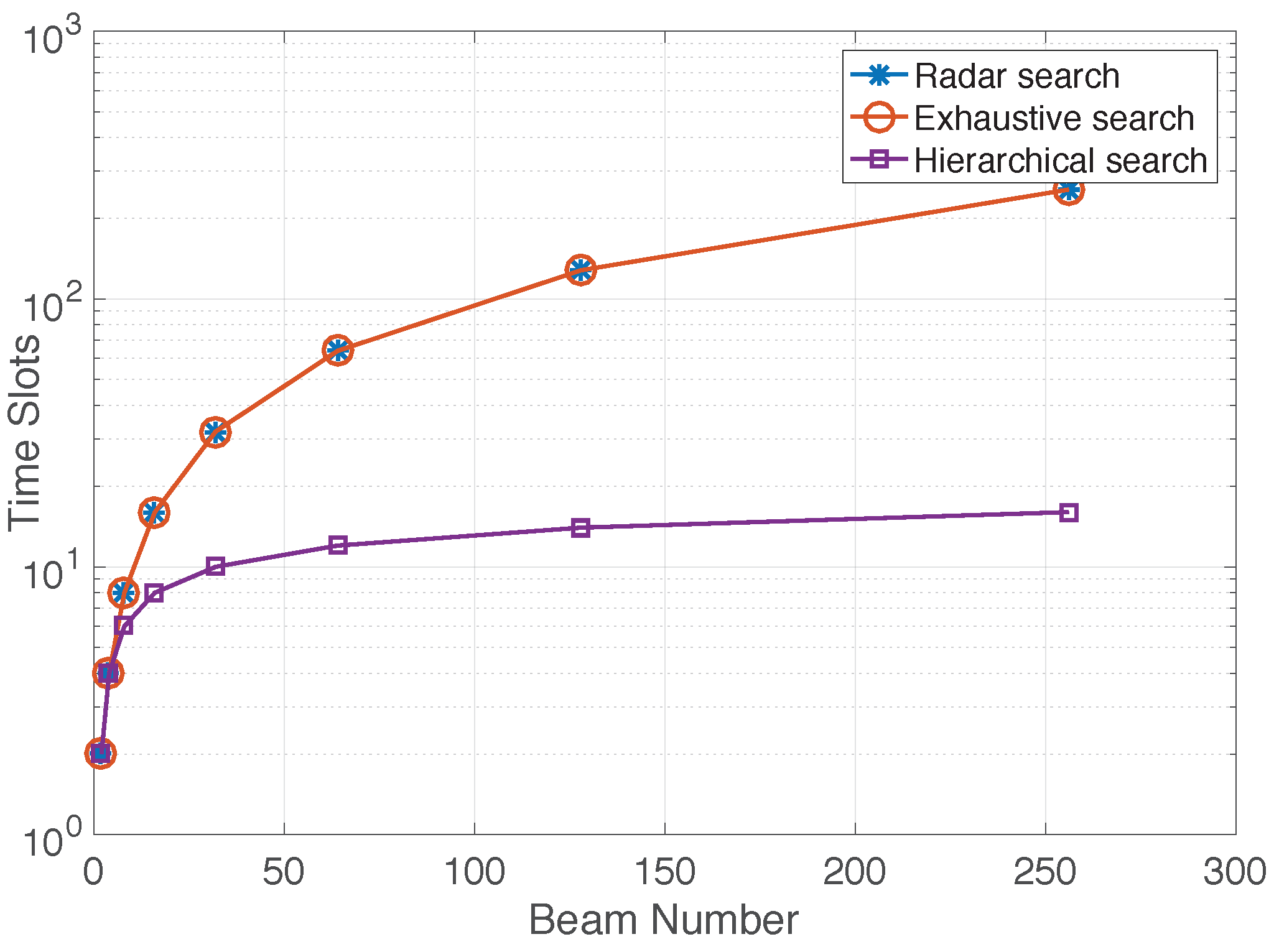
Figure 10.
Beam search time in MIMO radar system from the second base station.
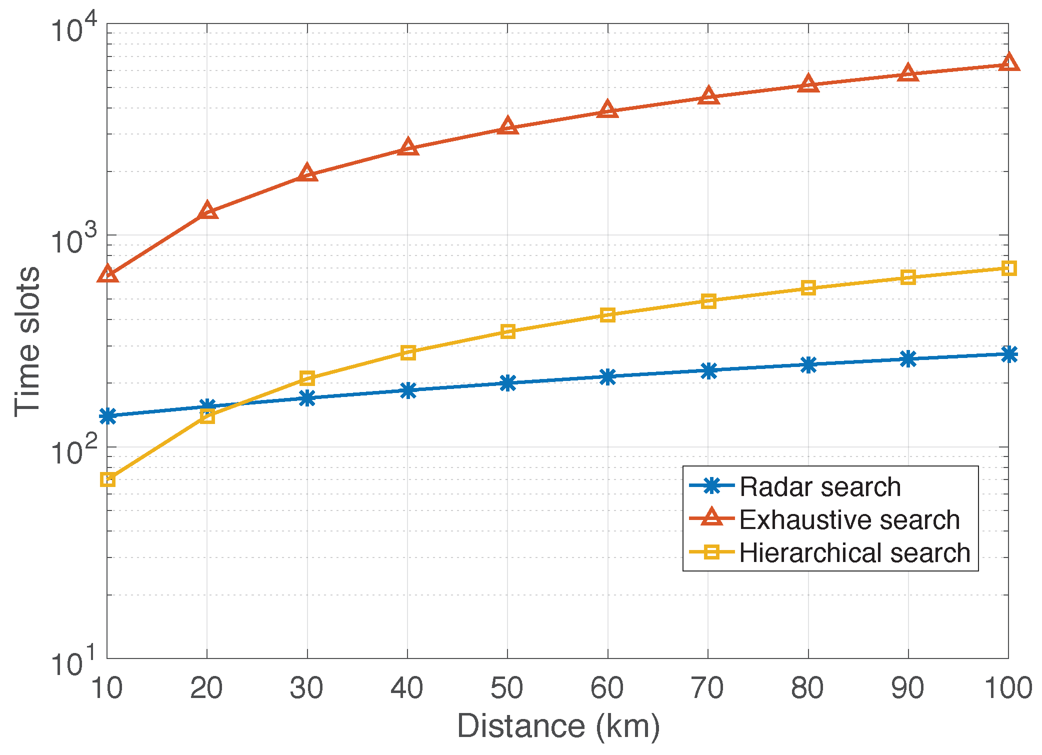
Figure 11.
Cell discovery time.

© 2018 by the authors. Licensee MDPI, Basel, Switzerland. This article is an open access article distributed under the terms and conditions of the Creative Commons Attribution (CC BY) license (http://creativecommons.org/licenses/by/4.0/).
Share and Cite
MDPI and ACS Style
Chen, Z.; Cao, Z.; He, X.; Jin, Y.; Li, J.; Chen, P. DoA and DoD Estimation and Hybrid Beamforming for Radar-Aided mmWave MIMO Vehicular Communication Systems. Electronics 2018, 7, 40. https://doi.org/10.3390/electronics7030040
AMA Style
Chen Z, Cao Z, He X, Jin Y, Li J, Chen P. DoA and DoD Estimation and Hybrid Beamforming for Radar-Aided mmWave MIMO Vehicular Communication Systems. Electronics. 2018; 7(3):40. https://doi.org/10.3390/electronics7030040
Chicago/Turabian StyleChen, Zhimin, Zhenxin Cao, Xinyi He, Yi Jin, Jingchao Li, and Peng Chen. 2018. "DoA and DoD Estimation and Hybrid Beamforming for Radar-Aided mmWave MIMO Vehicular Communication Systems" Electronics 7, no. 3: 40. https://doi.org/10.3390/electronics7030040
Note that from the first issue of 2016, this journal uses article numbers instead of page numbers. See further details here.