Article

Theoretical Tools for Relativistic Gravimetry, Gradiometry and Chronometric Geodesy and Application to a Parameterized Post-Newtonian Metric

1
SYRTE, Observatoire de Paris, PSL Research University, CNRS, Sorbonne Universités, UPMC University, Paris 06, LNE, 61 avenue de l’Observatoire, 75014 Paris, France
2
Czech Metrology Institute, Okružní 31, 63800 Brno, Czech Republic
*
Author to whom correspondence should be addressed.
Universe 2017, 3(1), 24; https://doi.org/10.3390/universe3010024
Submission received: 2 February 2017 / Revised: 8 March 2017 / Accepted: 8 March 2017 / Published: 13 March 2017

Abstract

:
An extensive review of past work on relativistic gravimetry, gradiometry and chronometric geodesy is given. Then, general theoretical tools are presented and applied for the case of a stationary parameterized post-Newtonian metric. The special case of a stationary clock on the surface of the Earth is studied.

1. Introduction

Physical geodesy is the study of the gravity field and of the figure of the Earth. One classical way to describe the “figure of the Earth” is to study the geoid, which is defined as one of the equipotentials of the Earth’s gravity (Newtonian) potential, which best coincides with the (mean) surface of the oceans. Therefore, heights are both physically and geometrically defined, and the objects of study of physical geodesy are both the physical Earth (underground masses, Earth and ocean topography, Earth rotation, etc.) and the gravitational field it generates. It implies a high intricacy between the three main pillars of geodesy—the determination of variations of Earth’s rotation, the geometric shape of the Earth and the spatial and temporal variations of its gravity field—but also with geodynamics and geophysics. Therefore, the International Association of Geodesy (IAG) established a “flagship” project named GGOS (Global Geodetic Observing System); it aims at connecting different communities in order to have a global understanding of the Earth system and to develop a common theoretical framework of high accuracy, which has to be based consistently (whenever this is necessary with respect to the measurement accuracy goal) on Einstein special and general relativity.
Many different techniques are used to monitor the Earth’s system: space geodetic techniques (VLBI, SLR/LLR, GNSS, DORIS, altimetry, InSAR and gravity missions), as well as terrestrial techniques (leveling, absolute and relative gravimetry, gradiometry and tide gauges). Moreover, the advent of space and ground transportable atomic clocks [1,2] will bring a completely new observable in geodesy: the direct measurement of gravity potential differences [3,4,5]. The high accuracy of most of these techniques necessitates their description in a relativistic framework. A review of several space geodetic techniques in a relativistic framework can be found in [6], as well as a detailed relativistic model for VLBI observations in [7].
In this article, we develop a general framework for relativistic geodesy with a focus on relativistic gravimetry, gradiometry and chronometric geodesy. An extensive review of these scientific fields is given in Section 2. In Section 3, we introduce some theoretical tools necessary to do the calculation of relativistic geodesy observables: the local frame, the geodesic equation and a theoretical description of the observables of relativistic gravimetry, gradiometry and chronometric geodesy. In Section 4, we calculate these observables for the special case of a parameterized post-Newtonian (PPN) metric of a stationary spacetime. Finally, in Section 5, we apply further our calculations to the case of a static clock relative to the Earth surface and give orders of magnitude.

2. Review of Past Work in Relativistic Gravimetry, Gradiometry and Chronometric Geodesy

Probably the first author who began the theoretical investigation of relativistic effects in gravimetry was Will [8]. He determined the Newtonian gravitational constant G as measured locally by means of Cavendish experiments in a parametrized post-Newtonian (PPN) framework [9,10,11], showing that in such a theoretical framework, an anisotropy appears in the locally measured G. This anisotropy implies a variation in gravimeter readings, such that Δ g / g = α ( Δ G / G ) , which have periods of 12 h sidereal time. By comparing with gravimeter data (measurements of “Earth tides”), he was able to rule out Whitehead’s theory, which predicted an effect 200-times larger than the experimental limit, as well as putting an upper limit on the parameter combination ( Δ 2 + ξ 1 ) to within three percent.

2.1. Chronometric Geodesy

The next application of relativistic geodesy to be explored, and probably the most interesting and promising, is the use of clocks to determine the spacetime metric. Indeed, the gravitational redshift effect discovered by Einstein must be taken into account when comparing the frequencies of distant clocks. Instead of using our knowledge of the Earth gravitational field to predict frequency shifts between distant clocks, one can revert the problem and ask if the measurement of frequency shifts between distant clocks can improve our knowledge of the gravitational field. To do simple orders of magnitude estimates, it is good to have in mind some correspondences:
1 meter Δ ν ν 10 16 Δ W 10 m 2 · s 2
where one meter is the height difference between two clocks, Δ ν is the frequency difference in a frequency transfer between the same two clocks and Δ W is the gravity potential difference between the locations of these clocks.
From this correspondence, we can already recognize two direct applications of clocks in geodesy: if we are capable to compare clocks to 10 16 accuracy, we can determine height differences between clocks with one-meter accuracy (leveling) or determine geopotential differences with 10-m 2 ·s 2 accuracy.
The first article to explore seriously this possibility was written in 1983 [12]. The article is named “chronometric leveling”. The term “chronometric” seems well suited for qualifying the method of using clocks to determine directly gravitational potential differences, as “chronometry” is the science of the measurement of time. However, the term “leveling” seems too restrictive with respect to all of the applications one could think of for using the results of clock comparisons. Therefore, we will use the term “chronometric geodesy” to name of the scientific discipline that deals with the measurement and representation of the Earth, including its gravitational field, with the help of atomic clocks. It is sometimes named “clock-based geodesy” or “relativistic geodesy”. However, this last designation is improper as relativistic geodesy aims at describing all possible techniques (including, e.g., gravimetry and gradiometry) in a relativistic framework. The natural arena of chronometric geodesy is the four-dimensional space-time. At the lowest order, there is proportionality between relative frequency shift measurements, corrected from the first order Doppler effect, and (Newtonian) gravity potential differences. To calculate this relation, one does not need the theory of general relativity, but only to postulate local position invariance. Therefore, if the measurement accuracy does not reach the magnitude of the higher order terms, it is perfectly possible to use clock comparison measurements, corrected for the first order Doppler effect, as a direct measurement of (the differences of) the gravity potential that is considered in classical geodesy. Comparisons between two clocks on the ground generally use a third clock in space. In this article, we calculate explicitly the higher order terms in the PPN formalism.
In his article, Martin Vermeer explores the “possibilities for technical realization of a system for measuring potential differences over intercontinental distances” using clock comparisons [12]. The two main ingredients are of course accurate clocks and a means to compare them. He considers hydrogen maser clocks. For the links, he considers a two-way satellite link over a geostationary satellite, or GPS receivers in interferometric mode. He has also to consider a means to compare the proper frequencies of the different hydrogen maser clocks. Today, this can be overcome by comparing primary frequency standards (PFS), which have a well-defined proper frequency based on a transition of cesium 133, used for the definition of the second. Secondary frequency standards, i.e., standards based on a transition other than the defining one, may nevertheless be used if the uncertainty in systematic effects has been fully evaluated, in the same way as for a PFS. It often happens that this evaluation can be done more accurately than for the defining transition. This is one of the purposes of the European project “International timescales with optical clocks” [13] (projects.npl.co.uk/itoc), where optical clocks based on different atoms are compared to each other locally and to the PFS. It is planned also to do a proof-of-principle experiment of chronometric geodesy, by comparing two optical clocks separated by a height difference of around 1 km using an optical fiber link. For more information about atomic clock relativistic time and frequency transfer, see [3,14].
Few authors have seriously considered chronometric geodesy. Following the Vermeer idea, the possibility of using GPS observations to solve the problem of the determination of geoid heights has been explored in [15]. They consider two techniques based on frequency comparisons and direct clock readings. However, they leave aside the practical feasibility of such techniques. The value and future applicability of chronometric geodesy has been discussed in [16], including direct geoid mapping on continents and joint gravity-geopotential surveying to invert for subsurface density anomalies. They find that a geoid perturbation caused by a 1.5-km radius sphere with a 20 percent density anomaly buried at a 2-km depth in the Earth’s crust is already detectable by atomic clocks of achievable accuracy. The potentiality of the new generation of atomic clocks has been shown in [17], based on optical transitions, to measure heights with a resolution of around 30 cm.
The possibility of determining the geopotential at high spatial resolution thanks to chronometric geodesy is thoroughly explored and evaluated in [18]. The authors consider the Alps-Mediterranean area, which comprises high reliefs and a land/sea transition, leading to variations of the gravitational field over a range of spatial scales. In such type of region, the scarcity of gravity data is an important limitation in deriving accurate high resolution geopotential models. Through numerical simulations, the contribution of clocks comparisons data in the geopotential recovery is assessed in combination with ground gravity measurements. It is shown that adding only a few clock data (around 30 comparisons) reduces the geopotential recovery bias significantly and improves the standard deviation by a factor of three. The effect of the data coverage and data quality are explored, as well as the trade-off between the measurement noise level and the number of data.

2.2. The Chronometric Geoid

Arne Bjerhammar in 1985 gave a precise definition of the “relativistic geoid” [19,20]:
“The relativistic geoid is the surface where precise clocks run with the same speed and the surface is nearest to mean sea level”
This is an operational definition, which has been translated in the context of post-Newtonian theory [21,22]. A different operational definition of the relativistic geoid has been introduced based on gravimetric measurements: a surface orthogonal everywhere to the direction of the plumb-line and closest to mean sea level. They call the two surfaces obtained with clocks and gravimetric measurements respectively the “u-geoid” and the “a-geoid”. They prove that these two surfaces coincide in the case of a stationary metric. In order to distinguish the operational definition of the geoid from its theoretical description, it is less ambiguous to give a name based on the particular technique to measure it. The term “relativistic geoid” is too vague, as Soffel et al. have defined two different ones. The names chosen by Soffel et al. are not particularly explicit, so instead of “u-geoid” and “a-geoid”, one can call them “chronometric geoid” and “gravimetric geoid”, respectively. There can be no confusion with the geoid derived from satellite measurements, as this is a quasi-geoid that does not coincide with the geoid on the continents [23]. Other considerations on the chronometric geoid can be found in [6,24,25].
We notice that the problem of defining a reference isochronometric surface is closely related to the problem of realizing terrestrial time (TT). This is developed in more detail in Section 3.4.
Recently, extensive work has been done aiming at developing an exact relativistic theory of Earth’s geoid undulation [26], as well as developing a theory of the reference level surface in the context of post-Newtonian gravity [27,28]. This goes beyond the problem of the realization of a reference isochronometric surface and tackles the tough work of extending all concepts of classical physical geodesy (see, e.g., [23]) in the framework of general relativity.

2.3. Gravimetry and Gradiometry

Following Will’s work, a PPN theory of gravimetric measurements was developed [21] taking into account only PPN parameters γ and β [11], with an accuracy of 10 11 g. In particular, they take into account the influence of all bodies in the Solar System and show that the relative second order corrections to gravimetric measurements (of order c 2 ) are of the form ( γ + 2 β 2 ) U / c 2 and ( γ 4 β + 3 ) U * / c 2 , where U and U * are respectively potentials related to the Earth and to all other Solar System bodies. It is claimed in [29] that it is impossible to measure the second order corrections to gravimetric measurements with two measurements, one at the South Pole and another one at the Equator, because of the errors induced by the uncertainty in the Earth’s flatness and mean equatorial radius. However, the study could go further and consider using more points at different latitudes.
In parallel, a theory of gradiometry measurements was developed, with a particular emphasis on measurements on-board a satellite and the feasibility of such measurements with superconducting gradiometers [30,31,32,33,34,35]. Recently, a test of the Chern–Simons modified gravity has been proposed with such an experiment [36], as well as a test of post-Newtonian physics of semi-conservative metric theories [37].

3. Theoretical Tools of Relativistic Geodesy

The theoretical background for relativistic geodesy is general relativity. We consider the spacetime as a Lorentzian manifold ( M , g ) of dimension four. We consider the components of the metric g μ ν to be given in an initial coordinate system ( x μ ) , defined in an open subset U . The infinitesimal interval d s 2 = g μ ν d x μ d x ν between two neighboring events is invariant under coordinate transformation.
All of the theoretical tools introduced in this section can be applied to any initial metric g , which is an exact or approximate solution of the Einstein equations and the components of which are given in any coordinate system. For applications in the vicinity of the Earth or in the Solar System, the International Astronomical Union (IAU) recommends to use respectively the GCRSor the BCRS, which both use harmonic coordinates. Explicit expressions of the metric components in these coordinate systems are given in [38]. Other approaches exist in this context based on generalized Fermi coordinates [39,40,41], or a perturbed Schwarzschild metric [42]. In the different context of a slowly-rotating astronomical object, the Kerr metric is used in [35].
The goal of this section is to describe a local experiment, such as a gravimeter, a gradiometer or a clock. To do so, we need to introduce a local frame and local coordinates adapted to the apparatus. There are several ways of introducing a local frame and coordinates [43]. From the principle of general covariance, any coordinate system can be used to describe the local measurements. Here, we use Fermi normal coordinates, which have the advantage of displaying “beautiful ties” to the Riemann curvature tensor, as well as to the physical acceleration and rotation of the observer. Indeed, the metric components in the Fermi normal coordinates can be expressed with the help of the Riemann tensor, as well as the accelerations and rotations measured by the observer. The metric components are the same as the ones of special relativity up to the first order in the local coordinates, such that they are “as Minkowskian as possible” [44,45]. As a consequence, the Fermi normal frame can be spatially fixed w.r.t. to an observer in any kinematical state.
The use of Fermi coordinates is not adapted for a self-gravitating body, the mass-energy of which contributes to the determination of the initial metric g when solving the Einstein equations. For this reason, harmonic coordinates are preferred and recommended for the definition and realization of relativistic celestial reference systems [25,38,46,47], where the frame origin can be centered on the center-of-mass of a massive body. However, a local apparatus is a test body that does not contribute to the background metric. Therefore, the definition of the Fermi coordinates is not a problem in this context. On the contrary, they have the advantage of separating the problem of the determination of the background metric and the observer trajectory in the initial coordinate system, on the one hand, and from the definition, description and modelization of the observables of the local experiment, on the other hand.
When using Fermi normal coordinates, unlike the harmonic coordinates approach, no matching procedure between the initial frame and the local frame is required in order to obtain the metric in the local frame, and the explicit coordinate transformations from the initial coordinate system to the local one are not required. Moreover, all frames obtained from a spatial rotation of the Fermi normal frame are still Fermi normal frames. This is not the case for the harmonic frame, as the harmonic gauge condition does not admit the rigidly rotating frames of [25] (Chapter 8). Therefore, obtaining a harmonic frame with a spatially-fixed axis w.r.t. the apparatus is a priori not possible. For all these reasons, we believe that using a Fermi frame and corresponding Fermi coordinates is a better choice in order to describe a local experiment. When possible, we will compare the results from both approaches: the Fermi normal frame and the harmonic frame.

3.1. Notations and Conventions

In this work, the signature of the Lorentzian metric g is ( + , , , ) . Greek indices run from zero to three, and Latin indices run from one to three. The partial derivative of A will be noted A , α = A / x α . We use the summation rule on repeated indices (one up and one down). η α β are the components of the Minkowski metric. The convention for the Riemann tensor is:
R μ α ν β = Γ μ α ν , β Γ μ α β , ν Γ μ ν σ Γ σ α β + Γ μ β σ Γ σ α ν
In this section, the indices for tensor components in the proper reference frame and the Fermi frame are denoted with a hat, i.e., A α ^ ( A 0 ^ , A ı ^ ) , as well as the partial derivative in the Fermi frame, i.e., A α ^ , ȷ ^ = A α ^ / X ȷ ^ .

3.2. The Local Frame

Let C be the observer world line; this world line is a timelike path ( d s 2 > 0 ). We call τ, the proper time, that is the integral value d τ d s 2 / c 2 along C between a chosen origin O and an arbitrary event P along C . The observer world line is parameterized with the proper time:
C : x μ = f μ ( τ )
The four-velocity is u μ = d f μ / d τ , and the four-acceleration is γ μ = D u μ / D τ , where D / D τ is the covariant differentiation along the world line C .

The Proper Reference Frame

We define the proper reference frame with coordinates ( X α ^ ) as in [45]. It is entirely determined by these two conditions:
  • On the observer world line, the temporal coordinate X 0 ^ / c of the proper reference frame is equal to the proper time τ of the observer, and the spatial coordinates X ı ^ are constant.
  • At first order in the new coordinates X α ^ , we want to recover the metric of an accelerated and rotating observer in special relativity [44].
The new coordinate system ( X α ^ ) is defined in an ad-hoc subset U C U , so that C is included in U C . We select P an event along C , so that x P μ = f μ ( τ ) . From Condition (1) we infer:
X P 0 ^ = c τ
where c is the velocity of light in vacuum.
The origin O is defined so that x O μ = f μ ( 0 ) , without loss of generality. The coordinate transformation from ( X α ^ ) to ( x μ ) is a diffeomorphism Y : X α ^ ( U C ) x μ ( U C ) . The partial derivatives of Y at point P are defined by the components of the Jacobian matrix:
e α ^ β = { x , α ^ β } P x ¯ , α ^ β
where x β = x β ( X α ^ ) are the components of Y , and the bar stands for the value of a function at point P (as P is arbitrary along the world line C , then the bar stands for the value of the function all along C , which means that all quantities with the bar over them are functions of the proper time τ). The inverse transformations follow:
e μ β ^ e α ^ μ = δ α ^ β ^
e μ β ^ e β ^ ν = δ μ ν
where δ is the Kronecker delta. We note that e 0 ^ μ = u μ / c .
For the sake of simplicity, X ı ^ ( C ) = 0 , i.e., the world line constitutes the spatial origin of the proper reference frame. The vector e 0 ^ μ is determined by the observer world line, while the vectors e ȷ ^ μ are chosen, such that ( e α ^ μ ) constitutes a basis of the tangent space for each event along C . ( e ȷ ^ μ ) is the spatial frame of the observer at event P. The transformation relations of the metric tensor are:
g α ^ β ^ = g μ ν x , α ^ μ x , β ^ ν
where g α ^ β ^ are the components of the metric tensor in the proper reference frame. For simplicity, we choose the vectors e α ^ μ , so that they form an orthonormal basis, so-called a tetrad, such that:
g α ^ β ^ ( C ) η α ^ β ^ = g μ ν ( C ) e α ^ μ e β ^ ν
where η α ^ β ^ is the Minkowski metric.
Then, it is shown in [45] that the metric in the proper reference frame can be written, up to first order in the new coordinates ( X α ^ ) :
d s 2 = 1 2 γ ȷ ^ X ȷ ^ + O X 2 c 2 d τ 2 + 2 Ω m ^ ȷ ^ X ȷ ^ + O X 2 d X m ^ c d τ + η l ^ m ^ + O X 2 d X l ^ d X m ^
where Ω α ^ β ^ is the antisymmetric rotation matrix defined with:
Ω α ^ β ^ = 1 2 g ¯ μ ν e α ^ μ D e β ^ ν D τ e β ^ μ D e α ^ ν D τ
and γ ȷ ^ = Ω ȷ ^ 0 ^ = g μ ν ( C ) e ȷ ^ μ γ ν . The function Ω α ^ β ^ ( τ ) defines the tetrad transport along the observer trajectory:
D e β ^ μ D τ = Ω α ^ β ^ e α ^ μ
where Ω α ^ β ^ = g ¯ σ ^ α ^ Ω σ ^ β ^ .
Moreover, we define the vector Ω k ^ , so that Ω ı ^ ȷ ^ = ε ı ^ ȷ ^ k ^ Ω k ^ , with ε ı ^ ȷ ^ k ^ the Levi–Civita symbol. Ω k ^ is the rotation of the observer spatial frame ( e ȷ ^ μ ) , as it can be measured with three gyroscopes. γ k ^ is the acceleration vector of the observer, as it can be measured with accelerometers. If Ω k ^ = 0 , the frame is Fermi–Walker transported; if Ω k ^ = 0 and γ k ^ = 0 , the frame is parallel transported (i.e., C is a geodesic).

The Fermi Normal Frame

Up to the second order in the coordinates, there is a certain choice of freedom to prolongate the coordinates lines of the proper reference frame. For the sake of mathematical simplicity, what is usually done is to define the Fermi normal frame, where the coordinate lines are taken as geodesics [45]. In the Fermi normal frame, the metric can be written:
d s 2 = 1 2 γ ȷ ^ X ȷ ^ + Ω α ^ ȷ ^ Ω α ^ k ^ + R ¯ 0 ^ ȷ ^ 0 ^ k ^ X ȷ ^ X k ^ + O X 3 c 2 d τ 2 + 2 Ω m ^ ȷ ^ X ȷ ^ + 4 3 R ¯ 0 ^ ȷ ^ m ^ k ^ X ȷ ^ X k ^ + O X 3 d X m ^ c d τ + η l ^ m ^ + 1 3 R ¯ l ^ ȷ ^ m ^ k ^ X ȷ ^ X k ^ + O X 3 d X l ^ d X m ^
A different approach is used in [24,25], where harmonic coordinates are used to build the local frame, named the topocentric reference frame. We prefer to name it the harmonic frame here as a reference to the corresponding harmonic coordinates. As a result, the metric components are very different when using harmonic coordinates (HC) [25] (see Equations (8.40) to (8.42)) from the ones using Fermi normal coordinates (FNC). The cross-component of the metric has no first order term in the HC, while in the FNC, the first order term depends on the observer rotation as in special relativity. Indeed, the harmonic frame is dynamically non-rotating [24,48], and therefore, it cannot be adapted to rotating observers. As in special relativity, there is no first order term in the spatial component of the metric in the FNC, while there is one when using the HC. The metric calculated in the HC in [24,25] is an expansion in both the local coordinates and c 1 (post-Newtonian approach), while there in no post-Newtonian expansion in the approach presented here. Finally, as a consequence of the equivalence principle, the metric components in the FNC do not depend on the chosen initial coordinate system, while the metric components in the HC do through the matching procedure. Moreover, the metric components in the FNC are expressed in terms of the Riemann tensor, acceleration and rotation of the observer, while in the HC, the metric components are expressed with non-tensorial quantities to be determined through the matching procedure.

3.3. Geodesic Equation in the Local Frame

The gravimetric and gradiometric observables can be deduced from the general dynamical equation of a test body written in the local frame:
d 2 X α ^ d λ 2 + c 2 Γ α ^ 0 ^ 0 ^ d τ d λ 2 + 2 c Γ α ^ 0 ^ ı ^ d τ d λ d X ı ^ d λ + Γ α ^ ı ^ ȷ ^ d X ı ^ d λ d X ȷ ^ d λ = F α ^ m Γ α ^
where λ is an affine parameter along the test body trajectory.
From [49], we can write it in all generality. We will consider the gravimeter/gradiometer to be made of components that are at rest with respect to the local frame, i.e., d X ı ^ / d λ = d 2 X ı ^ / d λ 2 = 0 , thanks to some local forces voluntarily applied to the apparatus components. In the local frame, we decompose a four-vector as ( V 0 ^ , V ı ^ ) ( V 0 ^ , V ) . Therefore, we deduce from [49] (Equation (25)):
Γ ı ^ = γ ı ^ + Ω × Ω × X ı ^ + η × X ı ^ + c 2 X l ^ R 0 ^ ı ^ 0 ^ l ^ + 1 c 2 ( γ · X ) γ ı ^ b · X Ω × X ı ^ 2 γ · Ω × X Ω × X ı ^ 1 3 γ k ^ R ı ^ l ^ k ^ m ^ X l ^ X m ^ 2 c X l ^ Ω × X k ^ R 0 ^ l ^ ı ^ k ^ + 2 X l ^ γ · X R 0 ^ ı ^ 0 ^ l ^ + c 2 2 R ı ^ l ^ m ^ 0 ^ ; 0 ^ + R ı ^ 0 ^ l ^ 0 ^ ; m ^ X l ^ X m ^ + O X 3
where b = d γ d τ + Ω × γ and η = d Ω d τ .
The geodesic equation using harmonic coordinates can be found in [24,25]. As the harmonic frame is dynamically non-rotating, all terms depending on rotation are absent. Moreover, the coefficients of the equation are found through the matching procedure; therefore, they depend on the choice of the initial metric and coordinate system. Then, it is not possible to compare the terms with Equation (14) here, which is more general.

3.3.1. Gravimetric Observables

We suppose that we apply a force to the gravimeter mass to keep it at the center of the local frame. Therefore, Equation (14) reduces to:
Γ ı ^ = γ ı ^
which is simply the physical acceleration of the local frame. We emphasize that here we suppose that the mass of the gravimeter is kept fixed at the center of the local frame. Therefore, the measured quantity is the force vector F applied to the mass in order to be still, such that Γ ı ^ = F ı ^ / m .

3.3.2. Gradiometric Observables

Suppose now that we have a two masses located in the direction e ȷ ^ of the spatial part of the local frame basis, at a distance l / 2 and l / 2 from the center of the frame. The local distance l is supposed to be constant here, e.g., by putting both accelerometers on a rigid structure. We define the local distance as the Euclidean distance calculated in terms of the coordinates of the local frame: l = ı ^ ( X ı ^ ) 2 . Then, we define the quantities measured by the differential accelerometer, or gradiometer, with:
Γ ı ^ ȷ ^ = 1 l Γ ı ^ τ , l 2 e ȷ ^ Γ ı ^ τ , l 2 e ȷ ^
By doing this, we suppose that the geometrical center of the gradiometer is at the origin of the local frame. From Equation (14), we deduce:
Γ ı ^ ȷ ^ = [ Ω × ( Ω × e ȷ ^ ) ] ı ^ + ( η × e ȷ ^ ) ı ^ + c 2 R 0 ^ ı ^ 0 ^ ȷ ^ + 1 c 2 γ ı ^ γ ȷ ^ + O l 2
In case of a free-falling and non-rotating gradiometer, one simply has:
Γ ı ^ ȷ ^ = c 2 R 0 ^ ı ^ 0 ^ ȷ ^ + O l 2

3.4. Clock Frequency Comparisons and Syntonization

The principle of clock frequency comparison is to measure the frequency of an electromagnetic signal with the help of the emitting clock, A, and then with the receiving clock, B. We obtain respectively two measurements ν A and ν B . However, in general, one measures the time of flight of the electromagnetic signal between emission and reception. Then, the ratio ν A / ν B can be obtained by deriving the time of flight measurements with respect to the time of reception.
Let S ( x α ) be the phase of the electromagnetic signal emitted by clock A. It can be shown that light rays are contained in hypersurfaces of constant phase. The frequency measured by A / B is:
ν A / B = 1 2 π d S d τ A / B
where τ A / B is the proper time along the world line of clock A / B . We introduce the wave vector k α A / B = ( α S ) A / B to obtain:
ν A / B = 1 2 π k α A / B u A / B α
where u A / B α = d x A / B α / d τ is the four-velocity of clock A / B . Finally, we obtain a fundamental relation for frequency transfer:
ν A ν B = k α A u A α k α B u B α
This formula does not depend on a particular theory and then can be used to perform tests of general relativity. It is needed in the context of relativistic geodesy, in order to calculate the gravitational potential difference between two clocks from the measurement of the ratio of the frequencies ν A / ν B .
Introducing v i = d x i / d t and k ^ i = k i / k 0 , it is usually written as:
ν A ν B = u A 0 u B 0 k 0 A k 0 B 1 + k ^ i A v A i c 1 + k ^ i B v B i c
From Equation (19), we deduce that:
ν A ν B = d τ B d τ A = d t d τ A d t B d t A d τ d t B
In the case of propagation in free space, if we suppose that the space-time is stationary, i.e., 0 g α β = 0 , then it can be shown that k 0 is constant along the light ray, meaning that k 0 A = k 0 B . Then, from Equations (22) and (23), we deduce that:
d t B d t A = 1 + k ^ i A v A i c 1 + k ^ i B v B i c
This term depends on how the signal propagates from A to B. For a free propagation in a vacuum, it is calculated up to order c 3 in [50], for the more general metric GCRS. Up to second order, it does not depend on the gravitational field, but only on the relative motion of the two clocks. It is simply the first order Doppler effect of order v c . At third order, there is a term of order G m r c 2 v c . It is less than 3 . 6 × 10 14 for a satellite and around 2 . 2 × 10 15 on the ground. In [51], the term (24) is calculated for the metric given later in Equations (27) to (29) up to the fourth order. It is stressed that the J 2 term of the expansion (30) in the third order term can amount to 1 . 3 × 10 16 for a satellite in low orbit.
If the signal propagates in an optical fiber, the term (24) has been calculated up to order c 3 in [52]. Up to second order, it does not depend on the gravitational field, as for the free propagation in vacuum. The first order term is due to the variation of the fiber length (e.g., due to thermal expansion) and of its refractive index. For a 1000-km fiber with refractive index n = 1 . 5 , this term is equal to 3 . 6 × 10 14 . The second order term is the derivative of the Sagnac effect, which is of order 10 19 or less for a 1000-km fiber. Finally, the third order term is of the order of 10 22 for a 1000-km fiber.
Syntonization is a different problem and is needed for the realization of coordinate time scales (such as TAI (Temps Atomique International)). It depends on the particular coordinate system chosen as a reference and is given by the derivative of proper time with respect to coordinate time. In a metric theory, one has c d τ = g α β d x α d x β , so that:
d τ d t ( u 0 ) 1 = g 00 + 2 g 0 i v i c + g i j v i v j c 2 1 / 2
where we defined the coordinate velocity v i = d x i / d t .
In the context of relativistic geodesy, this quantity is needed for the realization of the chronometric geoid. An isochronometric surface is a surface where all clocks beat at the same rate with respect to a reference coordinate time, such that the quantity (25) is constant. This reference coordinate time is usually taken as TT (terrestrial time), for which TAI is a realization, or TCG (Temps Coordonné géocentrique). The chronometric geoid is a reference isochronometric surface that should coincide up to some level with the classical geoid—a level surface of the gravity potential closest to the topographic mean sea level—so that a possible definition is:
d τ d ( T T ) = 1
TT is itself defined with respect to TCG with d ( T T ) / d ( T C G ) = 1 L G , where L G is a defining constant [38], chosen such that the reference isochronometric surface defined from TT (26) coincides with some level with the classical geoid.
An interesting problem is that the chronometric geoid will differ in the future from the classical geoid. Indeed, the value of the potential on the geoid, W 0 , depends on the global ocean level, which changes with time. In addition, there are several methods to realize that the geoid is “closest to the mean sea level”, so that there is yet no adopted standard to define a reference geoid and W 0 value (see, e.g., the discussion in [53]). Several authors have considered the time variation of W 0 (see, e.g., [54,55]), but there is some uncertainty in what is accounted for in such a linear model. A recent estimate over 1993 to 2009 is d W 0 / d t = 2 . 7 × 10 2 m 2 ·s 2 ·year 1 , mostly driven by the sea level change of +2.9 mm/year [55]. However, the rate of change of the global ocean level could vary during the next few decades, and predictions are highly model dependent [56]. Nevertheless, to state an order of magnitude, considering a systematic variation in the sea level of order 2 mm/year, different definitions of a reference surface for the gravity potential could yield differences in the frequency of order 2 × 10 18 in a decade. Comparisons of accurate clocks could therefore help in the future to establish a worldwide vertical datum.

4. Application to a Stationary PPN Metric Tensor

4.1. PPN Metric of an Isolated, Axisymmetric Rotating Body

In order to calculate the observables of relativistic geodesy with respect to the initial coordinate system and evaluate the higher order terms, we simplify the Earth metric. We consider that the Earth is a body in uniform rotation, isolated and axisymmetric. Moreover, in order to assess the potential of relativistic geodesy for general relativity tests, we generalize the metric to the so-called Will–Nordtvedt formalism [10,11]. This formalism contains ten parameters γ, β, ξ, α 1 , …, α 3 , ζ 1 , …, ζ 4 . The parameters α and γ are the usual Eddington–Robertson–Schiff parameters used to describe the classical tests of general relativity (=1 in GR), while other parameters measure preferred-location and preferred-frame effects and the violation of the conservation of total momentum. They are all zero in GR. Theories that possess conservation laws for total momentum, called “semi-conservative”, have five free PPN parameters (γ, β, ξ, α 1 , α 2 ). The PPN parameter γ has been constrained to | γ 1 | 2 . 3 × 10 5 using the Cassini spacecraft [57], β to | β 1 | 3 × 10 5 thanks to planetary ephemeris [58] and α 1 and α 2 to | α 1 | 6 × 10 6 and | α 2 | 3 . 5 × 10 5 thanks to refined values of Solar System planetary precessions [59]. Many other constraints have been put on PPN parameters, and a summary of these constraints can be found in, e.g., [11,60].
The assumptions done in this article to write the metric are simplistic, and for the analysis of a particular experiment, one should use a complete description of the metric around the Earth (see, e.g., [38,61]). This has been done in particular in the context of the detection of the Lense–Thirring effect in the Solar System (see, e.g., [62,63] and the references therein).
For the sake of simplicity, the only PPN parameters used here are γ, β and α 1 . w is the speed of the Earth center of mass with respect to a preferred rest frame, if one exists. We use a non-rotating geocentric reference system with initial coordinate system ( c t ; x i ) ( c t ; x ) . This case has been rigorously studied in [51]; the metric is stationary, and it is given by:
g 00 ( x ) = 1 2 c 2 W ( x ) + 2 β c 4 W 2 ( x ) + O ˜ 6
g 0 j ( x ) = 2 c 3 1 + γ + α 1 4 W ( x ) + 1 4 α 1 W ( x ) w + O ˜ 5
g i j ( x ) = δ i j 1 + 2 γ c 2 W ( x ) + O ˜ 4
where:
W ( x ) = G M r 1 n = 2 J n R r n P n ( cos θ ) ,
W ( x ) = G I ω × x 2 r 3 1 n = 1 K n R r n P n + 1 ( cos θ ) ,
r = x , θ is the angle between x and the axis of rotation of the Earth, ω its angular velocity, assumed constant, R its equatorial radius, the P n the Legendre polynomials, and the coefficients M, J 2 , …, J n , … and I, K 1 , …, K n , … are the multipole moments of the multipolar expansion of the potentials W and W , for which convergence is assumed. The angular momentum of the central body is J = I ω . The order of the metric expansion is:
O ˜ n = G M r c 2 n / 2
This is a practical notation: the term O ˜ n , when it is at the end of a sum, means O ( O ˜ n ) .

4.2. Clock Observables

From Equations (25) and the given metric (27) to (29), we calculate:
( u 0 ) 1 d τ d t = 1 1 c 2 W + 1 2 v 2 + 1 c 4 β 1 2 W 2 γ + 1 2 W v 2 1 8 v 4 + 2 γ + 1 + α 1 4 W · v + 1 2 α 1 W v · w + O 1 c 6
where v = | d x / d t | is the coordinate velocity; from which we deduce that:
( u 0 ) A ( u 0 ) B = 1 + 1 c 2 W A W B + 1 2 v A 2 1 2 v B 2 + 1 c 4 ( γ + 1 ) ( W A v A 2 W B v B 2 ) + 3 8 v A 4 1 8 v B 4 1 4 v A 2 v B 2 + 2 γ + 1 + α 1 4 ( W B · v B W A · v A ) + 1 2 α 1 w · ( v B W B v A W A ) 1 2 ( W A W B ) W A W B + 2 ( 1 β ) ( W A + W B ) + v A 2 v B 2 + O 1 c 6
This result coincides with the one of [51] when putting α 1 = 0 .

4.3. Gravimetry Observables

We find a tetrad that satisfies e 0 ^ α = u α / c and Equation (8) for the metric (27) to (29), valid for a general trajectory with coordinate velocity v i :
e 0 ^ 0 = 1 + 1 c 2 W + 1 2 v 2 + 1 c 4 β 3 2 W 2 + γ + 3 2 W v 2 + 3 8 v 4 2 γ + 1 + α 1 4 W · v 1 2 α 1 W v · w + O 1 c 6
e 0 ^ i = 1 c v i e 0 ^ 0
e ȷ ^ 0 = 1 c v j + 1 c 3 v j ( γ + 2 ) W + 1 2 v 2 g 0 j + O 1 c 5
e ȷ ^ i = δ i j + 1 c 2 1 2 v i v j δ i j γ W + O 1 c 4
where δ i j is the Kronecker symbol and g 0 j is given by (28). This tetrad coincides with the results found elsewhere for the the GR case, e.g., [47] (Equation (5.21)). Here, the tetrad is chosen such that it is identity at zeroth order: the spatial part is non-rotating with respect to distant stars as for the initial coordinate system. The case of a rotating tetrad does not change the gravimetry observable, as it is defined as a local quantity. However, it will be studied for the gradiometry observable.
As in Section 3.3, a four-vector is decomposed in the local frame defined in (35) to (38) as ( V 0 ^ , V ı ^ ) ( V 0 ^ , V ) , while it is decomposed as ( V 0 , V i ) ( V 0 , V ) in the initial coordinate system.
Then, we calculate the antisymmetric rotation matrix with Formula (10). We deduce from this matrix the physical acceleration experienced by the observer:
γ = a W + 1 c 2 ( γ + 2 β 2 ) W W + 2 γ + 1 + α 1 4 v × ( × W ) ( γ + 1 ) v 2 W + 2 γ + 3 4 ( v · W ) v + v 2 + ( γ + 2 ) W a + 1 2 α 1 W ( v · w ) w ( v · W ) + 1 2 ( v · a ) v + O 1 c 4
where a = d v / d t , and its rotation as measured with gyroscopes:
Ω = Ω LT + Ω dS + Ω Th + O 1 c 4
where:
Ω LT = 1 2 c 2 × g = 1 c 2 1 + γ + α 1 4 × W + α 1 4 W × w
Ω dS = 1 c 2 γ + 1 2 v × W
Ω Th = 1 2 c 2 v × γ
where ( g ) j c 3 g 0 j . This result coincides with the results found elsewhere (see, e.g., [64] (Equation (3.4.38)) for α 1 = 0 and [65] (Equations (5) to (7))).

4.4. Gradiometry Observables

Now, we consider a gradiometer fixed to the surface of the Earth and rotating together with the Earth. In this paper, we suppose a uniform rotation of the Earth and a stationary metric. Irregularities in the Earth rotation are not included here. We define a tetrad e ( α ) μ fixed to the gradiometer, such that the axes of the gradiometer are in the direction of the tetrad axes. This tetrad is related to the tetrad (35) to (38) aligned with the GCRS system by the following relations:
e ( 0 ) μ = e 0 ^ μ = u μ / c
e ( i ) μ = Λ ( i ) ȷ ^ e ȷ ^ μ
i.e., the spatial part is rotated by a matrix Λ ( i ) ȷ ^ S O ( 3 ) . This matrix is a function of a parameter along the gradiometer path, e.g., Λ ( i ) ȷ ^ ( t ) with t being the GCRS coordinate time. The gradiometer rotates together with the Earth surface, i.e., in cylindrical coordinates ( c t , ρ , ϕ , z ) related to the GCRS coordinates ( c t , x ) = ( c t , x , y , z ) as x = ρ cos ϕ ,   y = ρ sin ϕ ; its points move along orbits of the vector field t + ω ϕ where ω = d ϕ / d t is the angular velocity of the Earth surface. The tetrad e ( α ) μ is then Lie transported (to the order of interest) by this vector field. We obtain:
Λ ( i ) ȷ ^ ( t ) = B ( i ) ( k ) A ( k ) ȷ ^ ( t )
with:
A ( k ) ȷ ^ ( t ) = cos ω ( t t 0 ) sin ω ( t t 0 ) 0 sin ω ( t t 0 ) cos ω ( t t 0 ) 0 0 0 1 , B ( i ) ( k ) Λ ( i ) k ^ ( t 0 ) .
This leads to:
d Λ ( i ) ȷ ^ d t = Λ ( i ) k ^ ε ȷ ^ k ^ l ^ ω l ^
with ω l ^ = ( 0 , 0 , ω ) .
We can calculate the vector Ω ( j ) based on Formula (10) for the rotating tetrad e ( α ) μ . We obtain Ω ( j ) = ( Λ 1 ) ı ^ ( j ) Ω ı ^ = Λ ( j ) ı ^ Ω ı ^ with:
Ω = ω + 1 c 2 W + 1 2 v 2 ω + Ω LT + Ω dS + Ω Th + O 1 c 4
where Ω LT , Ω dS and Ω Th are defined respectively in (41) to (43).
Here, a four-vector is decomposed in the rotating local frame defined in (44) to (45) as ( V ( 0 ) , V ( i ) ) ( V ( 0 ) , V ˜ ) . For the first term of (17), we then obtain:
Ω ˜ × Ω ˜ × e ˜ ( n ) ( m ) = ( Λ 1 ) ı ^ ( m ) Λ ( n ) ȷ ^ [ Ω × ( Ω × e ȷ ^ ) ] ı ^ = Λ ( m ) ı ^ Λ ( n ) ȷ ^ [ Ω × ( Ω × e ȷ ^ ) ] ı ^
with:
[ Ω × ( Ω × e ȷ ^ ) ] ı ^ = [ ω × ( ω × e ȷ ^ ) ] ı ^ 1 + 1 c 2 2 W + v 2 + 2 ω ( ı ^ Ω ȷ ^ ) LT 2 δ ȷ ^ ı ^ ω k ^ Ω k ^ LT + 2 ω ( ı ^ Ω ȷ ^ ) dS 2 δ ȷ ^ ı ^ ω k ^ Ω k ^ dS + 2 ω ( ı ^ Ω ȷ ^ ) Th 2 δ ȷ ^ ı ^ ω k ^ Ω k ^ Th + O 1 c 4
= [ ω × ( ω × e ȷ ^ ) ] ı ^ 1 + 1 c 2 2 W + v 2 + 1 c 2 ( ω ( ı ^ ε j ) m n δ ȷ ^ ı ^ ω k ^ ε k m n ) 2 γ + 2 + α 1 2 W m , n + α 1 2 w m W , n + 1 c 2 ( ω ( ı ^ ε j ) m n δ ȷ ^ ı ^ ω k ^ ε k m n ) v m a n ( 2 γ + 2 ) W , n + O 1 c 4
The second term of (17) containing the angular acceleration is non-vanishing due to the term with vector w in the Lense–Thirring part of the angular velocity, which is not axially symmetric. The angular acceleration η ˜ = d Ω ˜ d τ is given as η ( j ) = ( Λ 1 ) ı ^ ( j ) η ı ^ = Λ ( j ) ı ^ η ı ^ with the components η ı ^ given by:
η = 1 c 2 α 1 4 ( w · W ) ω ( ω · W ) w + O 1 c 4
For the second term of (17), we then obtain:
( η ˜ × e ˜ ( n ) ) ( m ) = ( Λ 1 ) ı ^ ( m ) Λ ( n ) ȷ ^ ( η × e ȷ ^ ) ı ^ = Λ ( m ) ı ^ Λ ( n ) ȷ ^ ( η × e ȷ ^ ) ı ^ .
The third term of (17) can be obtained based on Formula (2.26) of [32]. This formula was derived for the metric (27) to (29) with w = 0 and general functions W ( x ) and W ( x ) ( U * ( x i ) and V j ( x i ) in the notation of [32]) and using the tetrad (35) to (38). The terms with w can be added by substitution of a corresponding function for V j . Thus, we get R ( 0 ) ( m ) ( 0 ) ( n ) = Λ ( m ) ı ^ Λ ( n ) ȷ ^ R 0 ^ ı ^ 0 ^ ȷ ^ with:
c 2 R 0 ^ ı ^ 0 ^ ȷ ^ = W , i j + 1 c 2 [ 2 ( β + γ 1 ) W ( γ + 1 ) v 2 W , i j + ( 2 β + 2 γ 1 ) W , i W , j γ δ i j | W | 2 + ( 2 γ + 1 ) v k v ( i W , j ) k γ δ i j v m v n W , m n + 2 γ + 2 + α 1 2 ( v k W k , i j v k W ( i , j ) k ) + α 1 2 ( v k w k W , i j v k w ( i W , j ) k ) + O 1 c 4
The last term of (17) can be expressed as γ ( m ) γ ( n ) = ( Λ 1 ) ı ^ ( m ) ( Λ 1 ) ȷ ^ ( n ) γ ı ^ γ ȷ ^ = Λ ( m ) ı ^ Λ ( n ) ȷ ^ γ ı ^ γ ȷ ^ , where using (39), we obtain:
1 c 2 γ ı ^ γ ȷ ^ = 1 c 2 a i W , i a j W , j + O 1 c 4
with a i being the centrifugal acceleration (circular motion is considered) of the center of the gradiometer with GCRS coordinates x c , y c given as a i = ω 2 ( x c , y c , 0 ) .

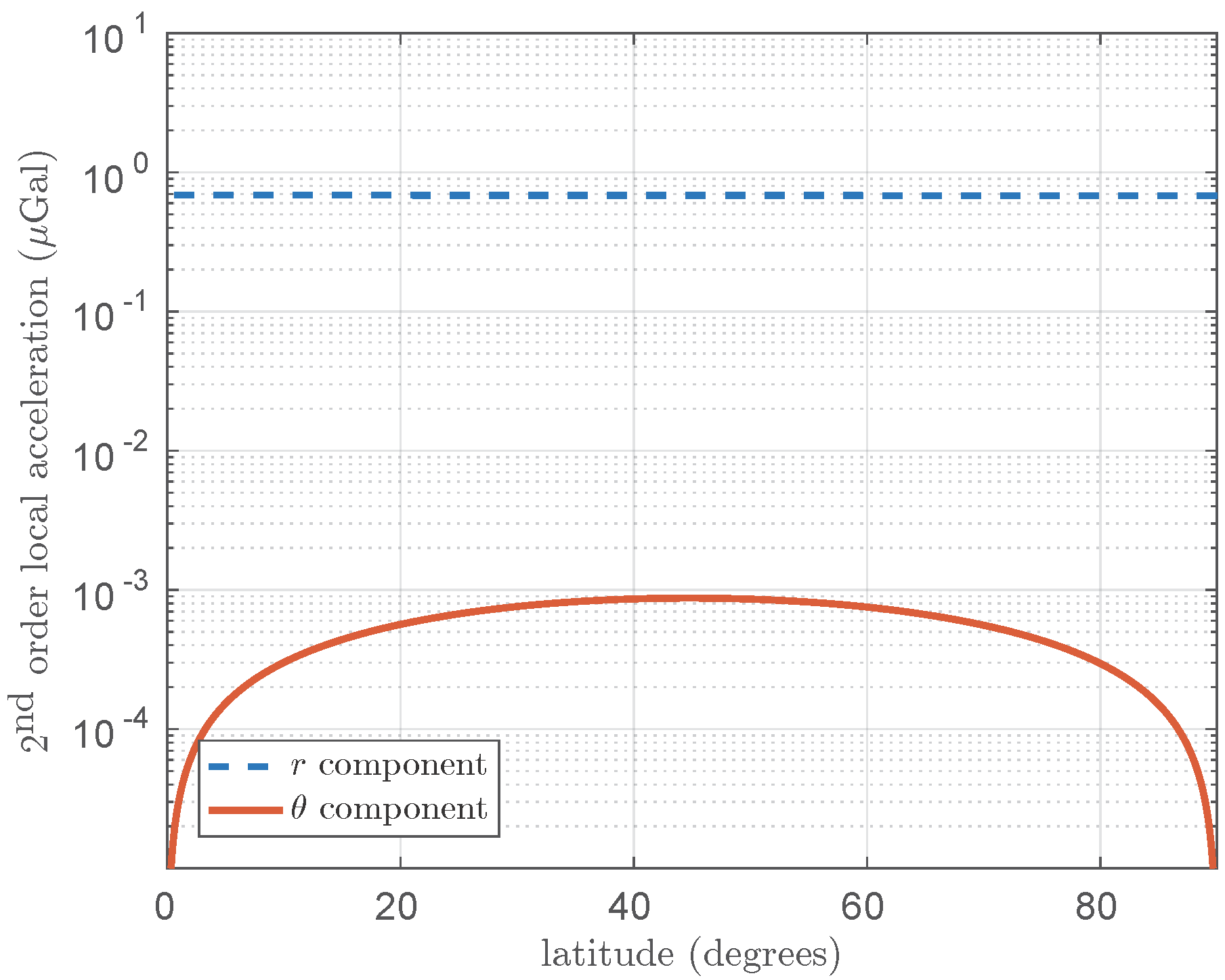
5. Orders of Magnitudes

Let us take a clock that is on the surface of the Earth, at rest in the rotating Earth frame. Then, in usual spherical coordinates ( r , θ , ϕ ) , one has:
v = v ϕ u ϕ = R ω sin θ u ϕ
a = a r u r + a θ u θ = R ω 2 sin θ sin θ u r + cos θ u θ
where R and ω are the Earth radius and angular velocity. Assuming that W = W ( r , θ ) , W = W ϕ ( r , θ ) u ϕ , γ = β = 1 and α 1 = 0 , we deduce from (39):
γ r = a r 1 + 1 c 2 v ϕ 2 + 3 W W , r 1 + 1 c 2 2 v ϕ 2 W + 4 c 2 v ϕ r ( r W ϕ ) r
γ θ = a θ 1 + 1 c 2 v ϕ 2 + 3 W W , θ r 1 + 1 c 2 2 v ϕ 2 W + 4 c 2 v ϕ r sin θ ( W ϕ sin θ ) θ
γ ϕ = 0
We take into account the gravitational potential up to second order:
W ( r , θ ) = G M r 1 J 2 R r 2 P 2 ( θ )
where P 2 ( θ ) = 1 2 3 cos 2 θ 1 is the Legendre function and J 2 1 . 083 × 10 3 is the Earth’s flatness. Moreover, we take into account only the monopole of the gravitational potential vector:
W ( r , θ ) = G J × r 2 r 3
where J = I ω is the Earth angular momentum. Attempts to measure the monopole of the gravitational potential vector with orbiting gyroscopes and satellites were performed in recent years (see, e.g., [66,67,68] and the references therein).
The order of magnitude of the fourth order relativistic effect in the absolute clock observable (33) is 2 × 10 19 , which is below the current clock accuracy. In terms of geoid height, it corresponds to 2 mm, which is also below the actual accuracy of the geoid determination (which is around 1 to 10 cm). The different contributions of non-linear terms to the geoid height are given in more detail in [6].
The second order contribution to the local acceleration γ is shown in Figure 1. One can see that the relativistic effects are below or just at the μGal level (1 Gal = 10 2 m·s 2 ), which is the accuracy of the best absolute gravimeters nowadays.
For gradiometry, the contribution of the relativistic effect is of the order of a few μ E (1 E = 1 eotvos = 10 9 s 2 ), when the accuracy of the best gradiometers to date is of the order of a few 100 μ E. However, it has been claimed that by integrating the effect over one year, it could become observable [32,69].

6. Conclusions

We have reviewed the literature of relativistic geodesy. We introduced the theoretical tools of relativistic geodesy and applied them for a stationary PPN metric. We applied the calculation to the case of a stationary clock on the Earth. Some interesting conclusions concerning post-Newtonian corrections are that:
  • differences between the chronometric geoid and the Newtonian geoid are of order 2 mm;
  • post-Newtonian corrections for gravimeters are below or just at the level of current accuracy of the best absolute gravimeters, which is about 1 μGal;
  • post-Newtonian corrections for gradiometers are below current accuracy, a few μ E, but could be measurable by integrating for a long time.

Acknowledgments

This work was partly funded by the European Metrology Research Programme (EMRP) within the SIB-55 ITOCproject. The EMRP is jointly funded by the EMRP participating countries within EURAMET and the European Union.

Author Contributions

P.D. and J.G. conducted all calculations and wrote the article together.

Conflicts of Interest

The authors declare no conflict of interest.

References

  1. Cacciapuoti, L.; Salomon, C. Space Clocks and Fundamental Tests: The ACES Experiment. Eur. Phys. J. Spec. Top. 2009, 172, 57–68. [Google Scholar] [CrossRef]
  2. Koller, S.B.; Grotti, J.; Vogt, S.; Al-Masoudi, A.; Dörscher, S.; Häfner, S.; Sterr, U.; Lisdat, C. Transportable Optical Lattice Clock with 7 × 10⁻¹⁷ Uncertainty. Phys. Rev. Lett. 2017, 118, 073601. [Google Scholar] [CrossRef] [PubMed]
  3. Delva, P.; Lodewyck, J. Atomic Clocks: New Prospects in Metrology and Geodesy. Acta Futura 2013, 7, 67–78. [Google Scholar]
  4. Flury, J. Relativistic Geodesy. J. Phys. Conf. Ser. 2016, 723, 012051. [Google Scholar] [CrossRef]
  5. Denker, H.; Timmen, L.; Voigt, C.; Weyers, S.; Peik, E.; Margolis, H.S.; Delva, P.; Wolf, P.; Petit, G. Geodetic methods to determine the relativistic redshift at the level of 10−18 in the context of international timescales—A review and practical results. J. Geod. 2017, in press. [Google Scholar]
  6. Müller, J.; Soffel, M.; Klioner, S.A. Geodesy and Relativity. J. Geod. 2007, 82, 133–145. [Google Scholar] [CrossRef]
  7. Soffel, M.; Kopeikin, S.; Han, W.B. Advanced Relativistic VLBI Model for Geodesy. J. Geod. 2016, 1–19. [Google Scholar] [CrossRef]
  8. Will, C.M. Relativistic Gravity in the Solar System. II. Anisotropy in the Newtonian Gravitational Constant. Astrophys. J. 1971, 169, 141–155. [Google Scholar] [CrossRef]
  9. Will, C.M. Theoretical Frameworks for Testing Relativistic Gravity. II. Parametrized Post-Newtonian Hydrodynamics, and the Nordtvedt Effect. Astrophys. J. 1971, 163, 611–628. [Google Scholar] [CrossRef]
  10. Will, C.M. Theory and Experiment in Gravitational Physics; Cambridge University Press: Cambridge, UK, 1993. [Google Scholar]
  11. Will, C.M. The Confrontation between General Relativity and Experiment. Living Rev. Relativ. 2014, 17, 4. [Google Scholar] [CrossRef] [PubMed]
  12. Vermeer, M. Chronometric Levelling; Technical Report; Finnish Geodetic Institute: Helsinki, Finland, 1983. [Google Scholar]
  13. Margolis, H.; Godun, R.; Gill, P.; Johnson, L.; Shemar, S.; Whibberley, P.; Calonico, D.; Levi, F.; Lorini, L.; Pizzocaro, M.; et al. International Timescales with Optical Clocks (ITOC). In Proceedings of the 2013 Joint European Frequency and Time Forum International Frequency Control Symposium (EFTF/IFC), Prague, Czech Republic, 21–25 July 2013; pp. 908–911.
  14. Petit, G.; Wolf, P.; Delva, P. Atomic Time, Clocks, and Clock Comparisons in Relativistic Spacetime: A Review. In Frontiers in Relativistic Celestial Mechanics—Volume 2: Applications and Experiments; Kopeikin, S.M., Ed.; De Gruyter Studies in Mathematical Physics; De Gruyter: Berlin, Germany, 2014; pp. 249–279. [Google Scholar]
  15. Brumberg, V.A.; Groten, E. On Determination of Heights by Using Terrestrial Clocks and GPS Signals. J. Geod. 2002, 76, 49–54. [Google Scholar] [CrossRef]
  16. Bondarescu, R.; Bondarescu, M.; Hetényi, G.; Boschi, L.; Jetzer, P.; Balakrishna, J. Geophysical Applicability of Atomic Clocks: Direct Continental Geoid Mapping. Geophys. J. Int. 2012, 191, 78–82. [Google Scholar] [CrossRef]
  17. Chou, C.W.; Hume, D.B.; Rosenband, T.; Wineland, D.J. Optical Clocks and Relativity. Science 2010, 329, 1630–1633. [Google Scholar] [CrossRef] [PubMed]
  18. Lion, G.; Panet, I.; Wolf, P.; Guerlin, C.; Bize, S.; Delva, P. Determination of a High Spatial Resolution Geopotential Model Using Atomic Clock Comparisons. J. Geod. 2017, 1–15. [Google Scholar] [CrossRef]
  19. Bjerhammar, A. On a Relativistic Geodesy. Bull. Geod. 1985, 59, 207–220. [Google Scholar] [CrossRef]
  20. Bjerhammar, A. Relativistic Geodesy; Technical Report NON118 NGS36; National Oceanic and Atmospheric Administration (NOAA): Silver Spring, MD, USA, 1986.
  21. Soffel, M.; Herold, H.; Ruder, H.; Schneider, M. Relativistic Theory of Gravimetric Measurements and Definition of the Geoid. Manuscr. Geod. 1988, 13, 143–146. [Google Scholar]
  22. Soffel, M.H. Relativity in Astrometry, Celestial Mechanics, and Geodesy; Springer: New York, NY, USA, 1989. [Google Scholar]
  23. Hofmann-Wellenhof, B.; Moritz, H. Physical Geodesy; Springer Science & Business Media: New York, NY, USA, 2006. [Google Scholar]
  24. Kopejkin, S.M. Relativistic Manifestations of Gravitational Fields in Gravimetry and Geodesy. Manuscr. Geod. 1991, 16, 301–312. [Google Scholar]
  25. Kopeikin, S.M.; Efroimsky, M.; Kaplan, G. Relativistic Celestial Mechanics of the Solar System; John Wiley & Sons: New York, NY, USA, 2011. [Google Scholar]
  26. Kopeikin, S.M.; Mazurova, E.M.; Karpik, A.P. Towards an Exact Relativistic Theory of Earth’s Geoid Undulation. Phys. Lett. A 2015, 379, 1555–1562. [Google Scholar] [CrossRef]
  27. Kopeikin, S.M.; Han, W.; Mazurova, E. Post-Newtonian Reference Ellipsoid for Relativistic Geodesy. Phys. Rev. D 2016, 93, 044069. [Google Scholar] [CrossRef]
  28. Kopeikin, S.M. Reference Ellipsoid and Geoid in Chronometric Geodesy. Front. Astron. Space Sci. 2016, 3, 5. [Google Scholar] [CrossRef]
  29. Iorio, L. On the Impossibility of Measuring the General Relativistic Part of the Terrestrial Acceleration of Gravity with Superconducting Gravimeters. Geophys. J. Int. 2006, 167, 567–569. [Google Scholar] [CrossRef]
  30. Mashhoon, B.; Theiss, D.S. Relativistic Tidal Forces and the Possibility of Measuring Them. Phys. Rev. Lett. 1982, 49, 1542–1545. [Google Scholar] [CrossRef]
  31. Theiss, D.S. A General Relativistic Effect of a Rotating Spherical Mass and the Possibility of Measuring It in a Space Experiment. Phys. Lett. A 1985, 109, 19–22. [Google Scholar] [CrossRef]
  32. Mashhoon, B.; Paik, H.J.; Will, C.M. Detection of the Gravitomagnetic Field Using an Orbiting Superconducting Gravity Gradiometer. Theoretical Principles. Phys. Rev. D 1989, 39, 2825–2838. [Google Scholar] [CrossRef]
  33. Li, X.Q.; Shao, M.X.; Paik, H.J.; Huang, Y.C.; Song, T.X.; Bian, X. Effects of Satellite Positioning Errors and Earth’s Multipole Moments in the Detection of the Gravitomagnetic Field with an Orbiting Gravity Gradiometer. Gen. Relativ. Gravit. 2014, 46, 1–14. [Google Scholar] [CrossRef]
  34. Xu, P.; Paik, H.J. First-Order Post-Newtonian Analysis of the Relativistic Tidal Effects for Satellite Gradiometry and the Mashhoon-Theiss Anomaly. Phys. Rev. D 2016, 93, 044057. [Google Scholar] [CrossRef]
  35. Bini, D.; Mashhoon, B. Relativistic Gravity Gradiometry. Phys. Rev. D 2016, 94, 124009. [Google Scholar] [CrossRef]
  36. Qiang, L.E.; Xu, P. Testing Chern-Simons Modified Gravity with Orbiting Superconductive Gravity Gradiometers: The Non-Dynamical Formulation. Gen. Relativ. Gravit. 2015, 47, 1–15. [Google Scholar] [CrossRef]
  37. Qiang, L.E.; Xu, P. Probing the Post-Newtonian Physics of Semi-Conservative Metric Theories through Secular Tidal Effects in Satellite Gradiometry Missions. Int. J. Mod. Phys. D 2016, 25, 1650070. [Google Scholar] [CrossRef]
  38. Soffel, M.; Klioner, S.A.; Petit, G.; Wolf, P.; Kopeikin, S.M.; Bretagnon, P.; Brumberg, V.A.; Capitaine, N.; Damour, T.; Fukushima, T.; et al. The IAU 2000 Resolutions for Astrometry, Celestial Mechanics, and Metrology in the Relativistic Framework: Explanatory Supplement. Astron. J. 2003, 126, 2687–2706. [Google Scholar] [CrossRef]
  39. Fukushima, T. The Fermi Coordinate System in the Post-Newtonian Framework. Celest. Mech. 1988, 44, 61–75. [Google Scholar] [CrossRef]
  40. Ashby, N.; Bertotti, B. Relativistic Perturbations of an Earth Satellite. Phys. Rev. Lett. 1984, 52, 485–488. [Google Scholar] [CrossRef]
  41. Ashby, N.; Bertotti, B. Relativistic Effects in Local Inertial Frames. Phys. Rev. D 1986, 34, 2246–2259. [Google Scholar] [CrossRef]
  42. Kostić, U.; Horvat, M.; Gomboc, A. Relativistic Positioning System in Perturbed Spacetime. Class. Quantum Gravity 2015, 32, 215004. [Google Scholar] [CrossRef]
  43. De Felice, F.; Bini, D. Classical Measurements in Curved Space-Times; Cambridge University Press: Cambridge, UK, 2010. [Google Scholar]
  44. Misner, C.W.; Thorne, K.S.; Wheeler, J.A. Gravitation; W. H. Freeman: New York, NY, USA, 1973. [Google Scholar]
  45. Delva, P.; Angonin, M.C. Extended Fermi Coordinates. Gen. Relativ. Gravit. 2012, 44, 1–19. [Google Scholar] [CrossRef]
  46. Kopejkin, S.M. Celestial Coordinate Reference Systems in Curved Space-Time. Celest. Mech. 1988, 44, 87–115. [Google Scholar] [CrossRef]
  47. Damour, T.; Soffel, M.; Xu, C. General-Relativistic Celestial Mechanics. I. Method and Definition of Reference Systems. Phys. Rev. D 1991, 43, 3273–3307. [Google Scholar] [CrossRef]
  48. Brumberg, V.A.; Kopejkin, S.M. Relativistic Reference Systems and Motion of Test Bodies in the Vicinity of the Earth. Nuovo Cimento 1989, 103, 63–98. [Google Scholar] [CrossRef]
  49. Li, W.Q.; Ni, W.T. Coupled Inertial and Gravitational Effects in the Proper Reference Frame of an Accelerated, Rotating Observer. J. Math. Phys. 1979, 20, 1473–1480. [Google Scholar] [CrossRef]
  50. Blanchet, L.; Salomon, C.; Teyssandier, P.; Wolf, P. Relativistic Theory for Time and Frequency Transfer to Order. Astron. Astrophys. 2001, 370, 320–329. [Google Scholar] [CrossRef]
  51. Linet, B.; Teyssandier, P. Time transfer and frequency shift to the order 1/c4 in the field of an axisymmetric rotating body. Phys. Rev. D 2002, 66, 024045. [Google Scholar] [CrossRef]
  52. Geršl, J.; Delva, P.; Wolf, P. Relativistic Corrections for Time and Frequency Transfer in Optical Fibres. Metrologia 2015, 52, 552. [Google Scholar] [CrossRef]
  53. Sánchez, L. Towards a Vertical Datum Standardisation under the Umbrella of Global Geodetic Observing System. J. Geod. Sci. 2012, 2, 325–342. [Google Scholar] [CrossRef]
  54. Burša, M.; Kenyon, S.; Kouba, J.; Šíma, Z.; Vatrt, V.; Vítek, V.; Vojtíšková, M. The Geopotential Value W0 for Specifying the Relativistic Atomic Time Scale and a Global Vertical Reference System. J. Geod. 2006, 81, 103–110. [Google Scholar] [CrossRef]
  55. Dayoub, N.; Edwards, S.J.; Moore, P. The Gauss–Listing Geopotential Value W0 and Its Rate from Altimetric Mean Sea Level and GRACE. J. Geod. 2012, 86, 681–694. [Google Scholar] [CrossRef]
  56. Jevrejeva, S.; Moore, J.C.; Grinsted, A. Sea Level Projections to AD2500 with a New Generation of Climate Change Scenarios. Glob. Planet. Chang. 2012, 80–81, 14–20. [Google Scholar] [CrossRef]
  57. Bertotti, B.; Iess, L.; Tortora, P. A Test of General Relativity Using Radio Links with the Cassini Spacecraft. Nature 2003, 425, 374–376. [Google Scholar] [CrossRef] [PubMed]
  58. Pitjeva, E.V.; Pitjev, N.P. Relativistic Effects and Dark Matter in the Solar System from Observations of Planets and Spacecraft. Mon. Not. R. Astron. Soc. 2013, 432, 3431–3437. [Google Scholar] [CrossRef]
  59. Iorio, L. Constraining the preferred frame α1, α2 parameters from Solar System planetary precessions. Int. J. Mod. Phys. D 2013, 23, 1450006. [Google Scholar] [CrossRef]
  60. Debono, I.; Smoot, G.F. General Relativity and Cosmology: Unsolved Questions and Future Directions. Universe 2016, 2, 23. [Google Scholar] [CrossRef]
  61. Soffel, M.; Frutos, F. On the Usefulness of Relativistic Space-Times for the Description of the Earth’s Gravitational Field. J. Geod. 2016, 90, 1345–1357. [Google Scholar] [CrossRef]
  62. Iorio, L.; Lichtenegger, H.I.M.; Ruggiero, M.L.; Corda, C. Phenomenology of the Lense-Thirring Effect in the Solar System. Astrophys. Space Sci. 2010, 331, 351–395. [Google Scholar] [CrossRef]
  63. Renzetti, G. History of the Attempts to Measure Orbital Frame-Dragging with Artificial Satellites. Open Phys. 2013, 11, 531–544. [Google Scholar] [CrossRef]
  64. Ciufolini, I.; Wheeler, J.A. Gravitation and Inertia; Princeton University Press: Princeton, NJ, USA, 1995. [Google Scholar]
  65. Angonin, M.C.; Tourrenc, P.; Delva, P. Cold Atom Interferometer in a Satellite: Orders of Magnitude of the Tidal Effect. Appl. Phys. B 2006, 84, 579–584. [Google Scholar] [CrossRef]
  66. Everitt, C.W.F.; Muhlfelder, B.; DeBra, D.B.; Parkinson, B.W.; Turneaure, J.P.; Silbergleit, A.S.; Acworth, E.B.; Adams, M.; Adler, R.; Bencze, W.J.; et al. The Gravity Probe B Test of General Relativity. Class. Quantum Gravity 2015, 32, 224001. [Google Scholar] [CrossRef]
  67. Iorio, L. An Assessment of the Systematic Uncertainty in Present and Future Tests of the Lense-Thirring Effect with Satellite Laser Ranging. Space Sci. Rev. 2009, 148, 363–381. [Google Scholar] [CrossRef]
  68. Renzetti, G. First Results from LARES: An Analysis. New Astron. 2013, 23–24, 63–66. [Google Scholar] [CrossRef]
  69. Paik, H.J. Detection of the Gravitomagnetic Field Using an Orbiting Superconducting Gravity Gradiometer: Principle and Experimental Considerations. Gen. Relativ. Gravit. 2008, 40, 907–919. [Google Scholar] [CrossRef]
Figure 1. Second order ( c 2 ) contributions to the local acceleration γ .
Universe 03 00024 g001

