1. Introduction
It has been suggested that our universe may not be the only universe but is part of a vast complex of universes by inflationary cosmology and string landscape. This is called a multiverse. Until recently, however, the multiverse idea has been a source of debate and criticized as a philosophical proposal because it is not testable. However, if quantum entanglement exists between two causally disconnected universes in the multiverse, the idea may be validated. In the multiverse, once inflation occurs, an infinite number of local universes with enormous diversity of environments can be produced as child universes in some parent universe. This is reminiscent of virtual particles which are created and annihilated continuously as entangled pairs in a vacuum state of quantum mechanics. Then our universe may have been nucleated as an entangled pair of universes coherently under certain causal mechanisms. Then our universe and the partner universe may have been separated off by the exponential expansion of space between us. Our parter universe may exist beyond the Hubble horizon afterwards. Since the quantum fluctuations as the origin of our universe may have been entangled with those of the unobservable universe out there, some effects of the entanglement with unobservable universe may appear in the CMB of our universe.
Recently, Maldacena and Pimentel calculated the entanglement entropy in a quantum field theory in the Bunch-Davies vacuum in de Sitter space [
1] in the course of progress in string theory. They showed that quantum entanglement can exist between two causally separated regions in de Sitter space. Then [
2] examined the spectrum of vacuum fluctuations by using the reduced density matrix in an open chart derived by [
1] and found that the quantum entanglement affects the shape of the spectrum on large scales comparable to or greater than the curvature radius. Since the scales larger than the curvature radius are beyond our current observable region, we now hope to find any signatures of entnaglmenet on smaller scales.
The research [
3,
4] showed that the entanglement of an initial state between two causally disconnected de Sitter spaces may remain even on small scales. Also the research [
5] explored that an initially entangled state between two scalar fields may produce its effect on the spectrum even on small scales. In this paper, we consider two universes in the inflationary multiverse. We simply assume the presence of entanglement and the initial state of our universe may not be settled down to the vacuum state during inflation. Assuming that one of them is our universe, we demonstrate how the difference between entangled and non-entangled initial states reflects on the spectrum of vacuum fluctuations. This has been done by us in [
6,
7] and this contribution is a report of the work.
This paper is organized as follows. In
Section 2, we construct an entanged state between two causally disconnected de Sitter spaces by using Bogoliubov transformations. In
Section 3, we consider an initially entangled state and calculate the spectrum of vacuum fluctuations in our universe. In
Section 4, we consider the same system with an initially non-entangled state and compute the spectrum. In
Section 5, we present another example that the quantum interference contributes to the spectrum directly for the non-entangled state. Our results are summarized in
Section 6.
2. Entangled States
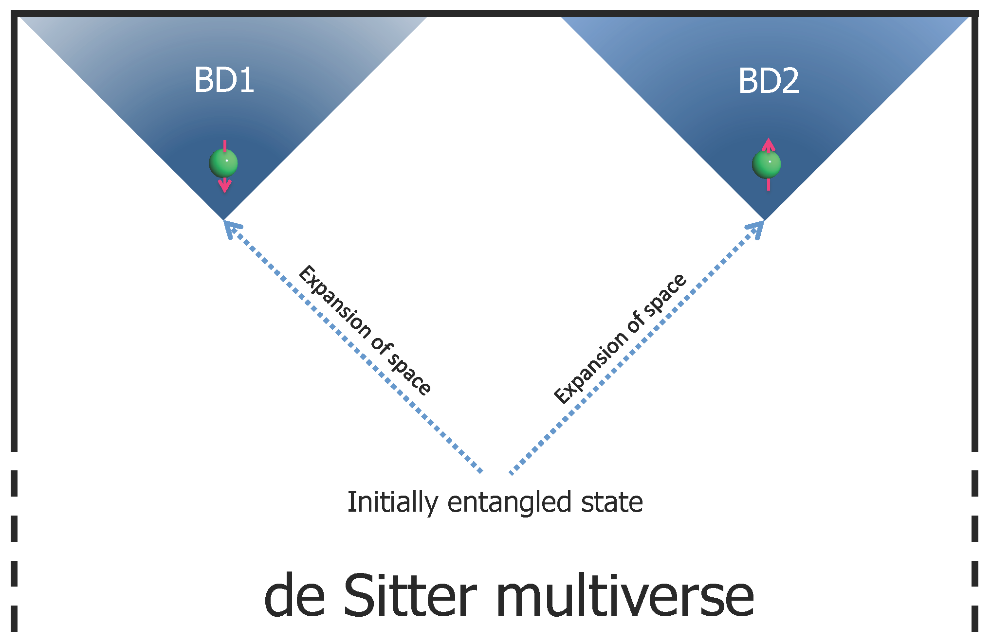
In order to discuss quantum entanglement between two causally disconnected de Sitter spaces (BD1 and BD2) depicted in
Figure 1, in this section, we show that entangled states are described as truncation of a squeezed state of pairs of
n-particles between BD1 and BD2. A quantum mechanical system consists of subsystems BD1 and BD2. The Hilbert space is a direct product
. We suppose that our universe is, say, BD2 and we have no access to BD1.
We consider a single mode
of a massless scalar field in de Sitter space. The vacuum state for each BD1 and BD2 is defined by different annihilation operators such as
where
and
are annihilation operators for BD1 and BD2. We omit the indices
for the state for simplicity unless there may be any confusion below. Let us consider a state
defined by Bogoliubov transformations that mix the operator of our partner universe
with the one of our universe
that is,
where
and
are the Bogoliubov coefficients that satisfy
. This state
is then written by
where
N is the normalization factor. This describes a squeezed state of pairs of
n-particles between BD1 and BD2. In fact, if we expand the exponent in
, we see the squeezed state clearly
where the states
and
are the vacuum and the one-particle states of the mode
in BD1 and similarly for BD2. This is called an entangled state of the
space. If we truncate the above at the one particle state order, we get the standard form of entanglement. Then the degree of entanglement expressed by the Bogoliubov coefficients may depend on the wavenumber
.
3. Initially Entangled State and Its Spectrum
In this section, we consider an initial state where the vacuum and one-particle states are entangled, as a simple example. We consider the flat slice for simplicity and assume that spatial curvature does not affect the point of discussion below. This example gives a clear difference in the spectrum whether BD1 and BD2 were initially entangled or not.
3.1. Initially Entangled State
We focus on a single mode with indices
of the scalar field as an initial state. Then an initially entangled state is described as truncation of Equation (
5) at the one particle state order such as
where the degree of entanglement expressed by the Bogoliubov coefficients
and
and the normalization
N in Equation (
5) is written by
and
.
is the probability to observe the state
.
is defined to conserve the probability
where
is a phase factor. When
, the state becomes maximally entangled state. The Bunch-Davies vacuum is recovered both for BD1 and BD2 when
and then
. In general, both
and
depend on the wavenumber
[
7,
8]. For simplicity, we omit the indices
unless there may be any confusion below.
3.2. Density Matrix
Since we have no access to the causally disconnected BD1, we have to trace out the degrees of freedom of BD1 and effectively to lose information about the inaccessible BD1. We derive the reduced density matrix of our universe BD2,
where
. Note that our quantum mechanical system becomes a mixed state by tracing out the inaccessible BD1 if the state is entangled.
3.3. Spectrum
Now we compute the spectrum of vacuum fluctuations by using the reduced density matrix (
8). For this purpose, in this section, we consider the mode function of a massless scalar field in de Sitter space as a simple example. However, as we will see, the following discussion is independent of the choice of the mode function.
The the spectrum of vacuum fluctuations is calculated by using the reduced density matrix (
8):
where we focused on a single mode with indices
.
In order to compute the above spectrum explicitly, we consider mode functions in our universe (BD2). For simplicity, we consider a massless minimally coupled scalar filed in de Sitter space. We expand the scalar field as
where
η is the conformal time and the mode expansion is given by
A vacuum state for BD2 is a state annihilated by
as defined in Equation (
1). The mode function
satisfies
Here a prime denotes derivative with respect to the conformal time
η and
where
a is the scale factor. The action for the mode
is,
The standard positive frequency function at far past
is
The spectrum of quantum fluctuation (
9) is calculated by using the mode function in (
11)
Putting the positive frequency mode Equation (
14) into the above, the spectrum after horizon exit (
) is evaluated as
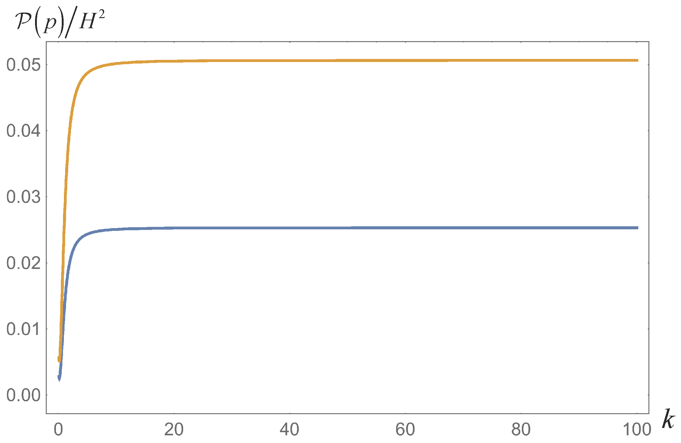
We see that the spectrum of the Bunch-Davies vacuum is recovered when
. The amplitude of spectrum is enhanced by factor 2 when the initial state is maximally entangled (
). The enhanced spectrum compared with the spectrum of the Bunch-Davies vacuum is plotted in
Figure 2.
4. Initially Non-Entangled State and Its Spectrum
In the previous section, we found that the quantum mechanical system becomes a mixed state by tracing out the inaccessible BD1 if the state is entangled. Then it turned out that the reduced density matrix consist of only diagonal elements. In this section, we consider an initially non-entangled state in order to clearly see the effect of entanglement and we will see that the off-diagonal elements due to quantum interference appear in the reduced density matrix. This effect may produce a modulation in the spectrum.
4.1. Initially Non-Entangled State
The one-particle states tend to enhance the spectrum compared with that of the Bunch-Davies vacuum, so the difference between the spectra for the entangled state and the vacuum is not solely due to the entanglement. Therefore, we consider a non-entangled state that includes one-particle states. Such a state is given by a direct product form
The above state gives the same probability for the vacuum and one-particle states as that for the entangled state (
6), if one focuses on either of the universe. This case contains extra two states
and
, if we compare it with Equation (
6).
4.2. Spectrum
We trace out the state of BD1 as we did in Equation (
8), then we find that the extra two states contribute to the spectrum of the form
Because the number of operators in the state does not match with that of operators
, those off-diagonal elements vanish. However, those off-diagonal elements give their effects on the spectrum in the form of the one point functions
and
. They produce a nonzero value
. Thus, in this case, we have to compute the spectrum with the variance
for the non-entangled state. The square of the mean value is found to be
Finally the spectrum becomes different from the one of entangled state Equation (
16),
We find the Bunch-Davies vacuum is recovered for .
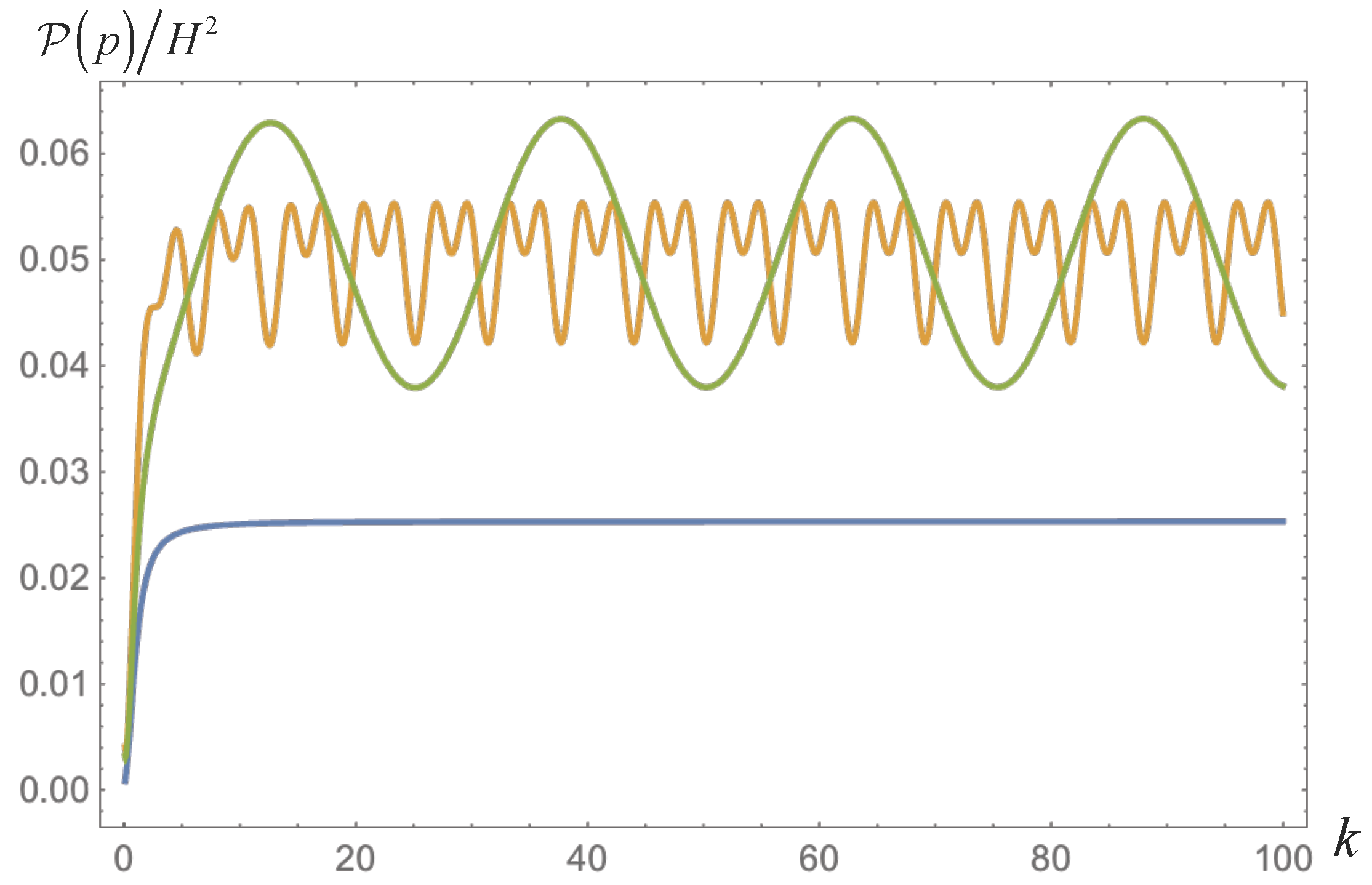
Since the off-diagonal elements represent quantum interference, we found that the quantum interference contributes to the spectrum in the form of variance. This effect distinguishes the spectrum of entangled state from the one of the non-entangled state. As we see in
Figure 3, the effect of the quantum interference may appear as oscillatory spectra because of the term proportional to
.
Although we presented the simplest case of entanglement, if we observe, further, the bispectrum or the higher order correlations such as ( for the bispectrum), the effect of quantum interference would contribute directly not only in the form of the variance and distinguish the spectrum between entangled and non-entangled states. As a simple demonstration, in the next section, we will see some direct contributions due to quantum interference by considering the states with two-particle discrepancy.
5. Entangled and Non-Entangled States with Two-Particle Discrepancy
In the multiverse, it would be possible to nucleate a pair of universes, one in vacuum and the other with two-particle states. We consider an initially entangled state between states with two-particle discrepancy, which is expressed as
The spectrum after tracing out the BD1 is then computed as
where we used
Note that the Bunch-Davies vacuum is recovered for
. The corresponding non-entangled state with a direct product form becomes
If we trace out the BD1, then we find that the extra two terms in the non-entangled state give the off-diagonal elements such as
Notice that the quantum interference enters into the spectrum of non-entangled state. The spectrum is then found to be
Because
after horizon exit (
), the spectrum becomes
We see that the Bunch-Davies vacuum is recovered for and then . Also, an oscillatory spectrum may appear because of the term proportional to when θ depends on k.
6. Summary
In this work, we discussed that cosmological implications of quantum entanglement between two causally disconnected de Sitter spaces in the multiverse. As a simple example, we considered that our universe (BD2) and our partner universe (BD1) was nucleated as an entangled state initially, each either with one-particle states or in vacuum. After deriving the reduced density matrix of BD2 by tracing out the degrees of freedom of BD1, we examined the spectrum of vacuum fluctuations for BD2. It is found that the quantum mechanical system becomes a mixed state by tracing out the inaccessible BD1, and the spectrum consists of only diagonal elements. As a result, the spectrum was enhanced depending on the degree of entanglement if we compared it with the spectrum of the Bunch-Davies vacuum.
Since such an enhancement was found to be due to the one-particle states included in the initially entangled state, we next considered a corresponding initially non-entangled state in order to see the effect of entanglement solely. We derived the reduced density matrix for BD2 similarly and examined the spectrum again. Since the state is non-entangled, the quantum mechanical system remains a pure state even after tracing out the inaccessible BD1. As a result, the off-diagonal elements which describe quantum interference come in the spectrum and we found that a modulation may appear in the spectrum due to the quantum interference. This may give rise to possibility that the quantum interference distinguishes whether our universe is initially entangled state or non-entangled state. Since the off-diagonal elements may contribute to the spectrum directly, we also mentioned that such modulation may contribute to the spectrum in different forms if we consider the bispectrum or higher order correlations. We demonstrated it by using an entangled states with two-particle discrepancy was considered.
As the entangled state is described as truncation of a squeezed state of pairs of
n-particles, the degree of entanglement
may have a scale dependence [
7,
8]. Thus the modulation due to the quantum interference may have oscillatory behaviors. However, we should not be confused the oscillatory spectra as an effect of entanglement. Oscillatory spectra are always possible for non-Bunch Davies vacua which can be obtained by the Bogoliubov transformation between two entangled Bunch-Davies vacua [
5,
7]. But such oscillations are different from those due to quantum interference. In terms of the coefficient
in Equation (
7), the entangled state may have an oscillatory spectrum if
is oscillatory, while an oscillation may appear for the non-entangled state even if
has no oscillation but if its phase
θ depends on scales.
Acknowledgments
This work was supported by IKERBASQUE, the Basque Foundation for Science and the Basque Government (IT-979-16), and Spanish Ministry MINECO (FPA2015-64041-C2-1P).
Conflicts of Interest
The authors declare no conflict of interest.
References
- Maldacena, J.; Pimentel, G.L. Entanglement entropy in de Sitter space. High Energy Phys. Theory 2013, 2013, 038. [Google Scholar] [CrossRef]
- Kanno, S. Impact of quantum entanglement on spectrum of cosmological fluctuations. J. Cosmol. Astropart. Phys. 2014, 2014, 029. [Google Scholar] [CrossRef]
- Kanno, S.; Shock, J.P.; Soda, J. Entanglement negativity in the multiverse. J. Cosmol. Astropart. Phys. 2015, 2015, 015. [Google Scholar] [CrossRef]
- Kanno, S.; Shock, J.P.; Soda, J. Quantum discord in de Sitter space. Phys. Rev. D 2016, 94, 125014. [Google Scholar] [CrossRef]
- Albrecht, A.; Bolis, N.; Holman, R. Cosmological Consequences of Initial State Entanglement. High Energy Phys. Theory 2014, 2014, 093. [Google Scholar] [CrossRef]
- Kanno, S. Cosmological implications of quantum entanglement in the multiverse. Phys. Lett. B 2015, 751, 316–320. [Google Scholar] [CrossRef]
- Kanno, S. A note on initial state entanglement in inflationary cosmology. Europhys. Lett. 2015, 111, 60007. [Google Scholar] [CrossRef]
- Kanno, S.; Sasaki, M.; Tanaka, T. Vacuum state of the Dirac field in de Sitter space and entanglement entropy. J. High Engergy. Phys. 2017, 1703, 068. [Google Scholar] [CrossRef]
© 2017 by the author. Licensee MDPI, Basel, Switzerland. This article is an open access article distributed under the terms and conditions of the Creative Commons Attribution (CC BY) license ( http://creativecommons.org/licenses/by/4.0/).

