Long-Lived Levels in Multiply and Highly Charged Ions


Fakultät für Physik und Astronomie, Astronomical Institute Ruhr University Bochum (AIRUB), Ruhr-Universität Bochum, 44780 Bochum, Germany
Atoms 2024, 12(3), 12; https://doi.org/10.3390/atoms12030012
Submission received: 28 December 2023
/
Revised: 19 February 2024
/
Accepted: 21 February 2024
/
Published: 23 February 2024
(This article belongs to the Section Atomic, Molecular and Nuclear Spectroscopy and Collisions)
Abstract
:Atoms and ions remain in some long-lived excited levels for much longer than in typical “normal” levels, but not forever. Various cases of this so-called metastability that occur in multiply or even highly charged ions are discussed in a tutorial review, as well as examples of atomic lifetime measurements on such levels, their intentions, and some present and future applications.
1. Introduction
Energy (E) levels of a finite lifetime have a finite width because of Heisenberg’s uncertainty principle, . Consequently, the ground state of an atom or ion is sharp because it is stable (it does not decay). Any excited level will eventually decay by whatever mechanism. Classical physics describes the energy loss of the atom in analogy to a mechanical oscillator and uses an exponential decay curve. This description works surprisingly well. However, since the duration of the quantum jump of a single atom may be arbitrarily short, the exponential curve does not describe a single atom but the energy loss of a sample of atoms (due to the radiative decays of numerous excited atoms); the exponential features a decay constant that is the inverse of the mean level lifetime. The Fourier transform of the exponential is a peaked curve of Lorentzian shape. The width of this Lorentzian relates to the decay rate. In the analog case of a periodically forced macroscopic oscillator, the response curve amplitude features a resonance (if the damping is not too strong); the resonance curve shows some widening because of the damping and is narrowest for the smallest damping. Intuitively, the apparent analogy of a macroscopic phenomenon and a quantum one is striking.
With high-resolution spectroscopy, it is possible to observe the natural line width of spectral lines, especially if the atomic level is particularly short-lived. Very-high-resolution spectroscopy often strives to measure spectra and associated phenomena with a resolving power that is even better and that permits observations finer than the natural line width. There are numerous successful experiments of this kind, most often using lasers. Does this mean that all is understood in terms of the above analogy of atoms and mechanical oscillators? Not quite—neither mechanics nor electrodynamics nor quantum mechanics explain why excited atoms decay in the way they do. Arguments have been brought up as to why not even the exponential decay should be evident from first principles. Apparently one has to consider the energy fluctuations of the physical vacuum in which real and virtual photons are produced and absorbed to understand why “spontaneous emission” takes place at all, in analogy to stimulated emission, but induced by interactions with real or virtual background photons.
While I enjoy the concept, the details are beyond my physics horizon. The same is true for many of the theoretical recipes applied to compute atomic decay rates due to this or that specific interaction. Fortunately, little of the detail is necessary to discuss the phenomena associated with most atomic level lifetimes, and in this tutorial review I will do without. (I intend to cite a few theoretical references, but the gist of the discussion should be understandable without the topical detail knowledge). However, be assured that proper theoretical treatments have been developed, and in most cases, these yield lifetime results that are compatible with the results of measurements. This success builds confidence for the many lifetime data that the experiment has not covered and in many cases may never be able to treat with useful accuracy. Still, some conflicts indicate the need to improve theoretical and/or experimental techniques or hint at factors outside the present models.
Experience (experiment, theory) shows that the characteristic time in the decay of a given atomic excitation level may lie in a wide range, from, say, 10 s to years (10 s) (see discussion and references in [1]). For example, the electric-dipole () transition rate of the Lyman- transition in the H-like ion of Fermium (), with all but one electron removed, can be calculated (neglecting relativistic effects) to yield a 2p level lifetime of about 1.6 s. In contrast, one of the longest atomic lifetimes measured so far is 49,800,000 s (≈1.6 years) for the 4f136s2 F level in Yb II (Yb) [2], which decays only by an electric octupole () transition. In nuclear physics, the corresponding lifetime range is even wider if one includes radioactivity, which lets the composition of the nucleus change. There are radioactive isotopes with ground-state lifetimes that reach into the range of billions of years. The present discussion is limited to excitations of the electron shell. In atoms and ions, only the ground state is stable, while most excited levels are rather short-lived (“unstable”), and a minority appears long-lived, or “almost stable”, in the time frame of a given experiment. The latter are often called “metastable”.
For many decades, metastable levels in atoms and low-charge ions have served a variety of technical roles, from fluorescent lighting tubes and HeNe lasers to surface etching by gas discharges or skin disinfection by plasmas. These technical aspects are outside the scope of this tutorial. Here, I want to discuss various reasons for the longevity of certain levels in multiply charged ions and their role in physics studies. The underlying atomic physics is part of the standard physics curriculum and has been described well and extensively in textbooks for almost a century. The goal of the text is achieved with the reader becoming more familiar with the concept of metastability in atoms and learning where to look for more detailed information.
2. What Is “Metastability”?
My personal introduction to the field was somewhat haphazard and demonstrates that anyone may encounter the topic: at several nuclear physics institutes (with rather limited atomic spectroscopy expertise) a curious observation was made of optical emission in a Geiger–Müller-type gas discharge: the purer the gas, the brighter the light. In my thesis experiment with Ar, the brightest emission occurred at wavelengths 104.8 nm and 106.7 nm, from the resonance and intercombination lines of neutral Ar. The Ar I resonance level 3s3p4s P has a level lifetime of about 2 ns [3]; there is also a P level with a lifetime of about 7 ns (the rare gases are usually described by other coupling schemes, but coupling is chosen here for its conceptual transferability to many other ions discussed below). These level lifetimes are both in the nanosecond range that is typical for levels with electric dipole () decays of atoms towards their ground state. However, the light emission observed from a μs-duration high voltage pulse exciting the gas lasted for many microseconds after. Obviously, this lasting emission did not reflect the natural level lifetime of the atomic levels observed decaying, nor did the non-exponential light curves reveal any other specific levels. My eventual interpretation concluded that sufficiently many atoms were excited to the 3s3p4s P levels, which on their own cannot decay by decays to the 3s3p S ground level. A (hypothetical) transition would require a (probably non-existent) monopole transition, and a decay needs a magnetic quadrupole () transition, the computed rate of which is certainly very low (and now, half a century later, this transition is still not listed in the ever-so-useful NIST online database [3]). Thus, both of these levels must be long-lived and almost stable, which is commonly labeled as “metastable”: not quite stable. I will return to this label below.
The delayed ultraviolet (UV) emission of some of the contaminants of the discharge gas (such as residual water vapor) has been connected with energy stored by long-lived excited levels (presumably of Ar), which transfer their excitation collisionally to other atoms and molecules (see discussion in [4]). If the density of such metastable atoms is sufficiently high, it should happen that pairs of them collide, and with a certain probability their excitation energies might be reshuffled so that one or both atoms end up in one of the short-lived levels, and then the atoms can decay radiatively. Two excited collision partners usually are rarer than one and a ground state atom, but the excitation energies are much closer to resonance and the interaction cross sections should be larger. The observed extreme ultraviolet (EUV) light curves in my experiment thus should reflect the density variation of metastable Ar atoms in the gas discharge after the excitation has ended [5]. My (nuclear physics) boss told me that “this can’t well be the case”. However, I am by far not the only person to have conceived such processes, and in other laboratories such excitation-sharing processes have since been studied in well-controlled detail.
Other long-lived levels in atoms or low-charge state ions play important roles in fluorescent lighting or in the HeNe laser: in the latter, energetic electrons excite and thus populate the long-lived He I 1s2s S and S levels of the He fraction of the gas mixture, which in turn (by collisions) pass their excitation onto Ne atoms. After some internal re-shuffling this almost selective excitation of Ne then results in the population inversion sought for the lasing process. (Actually, in the above example on Ar, the collisions take place among metastables, whereas in the HeNe laser plasma, only one collision partner (He) is in a long-lived state. In both cases, a collision energy in the meV range enables the energy match of the intrinsically different level energies—room temperature corresponds to about 25 meV). In other plasmas, excited long-lived rare-gas particles may transport “chunks of energy” (excitation energies on the order of 10 eV) into spatial regions that need to be kept free from charged contaminants. An excited rare gas atom may deliver its excitation energy to a surface. Delivering the internal energy to the material, the atom reverts into an inert ground state atom that will leave again and thus not perturb the chemical composition of the target substrate. The inner excitation of ions also modifies the sputtering yield when energetic such ions bombard a surface. These technical processes have been studied and applied for decades. They are not the subject of this tutorial. However, the above examples show that my topic is actually not exotic, but closely related to common technical applications in our laboratories and households.
Let me return to the concept of metastability. In classical physics, a ball resting in a valley is considered to be in gravitational confinement. After small perturbations, the ball returns to the lowest position in the potential, which is considered a stable one. A ball carefully placed on top of a hill does not move on its own; only after a perturbation does it move away and not return to its previous temporary resting place; this situation is “unstable upon perturbation”. Since the quiet resting may last until some external trigger happens, it is also called metastable—not as unstable as any position on the slopes of the hill, but at least seemingly stable for a while. In atoms, the only stable level is the ground level. By interaction with a radiation field, including the virtual photons of the quantum vacuum, any other level is not truly stable, even as some excited levels are extremely long-lived. Taking electric dipole () decays as “fast”, any selection rule that hinders decays may cause some degree of longevity in an excited level. For example, levels or levels above a ground state, as in the above example of Ar, qualify for (some degree of) metastability. This concept evidently points to levels that are much longer lived than others in the same atomic system, but the actual level lifetime may still be absolutely short, long, or very long. Metastability in atoms is a relative measure, not a sharply defined physical characteristic. I will use it interchangeably with “longevity”. There is no specific absolute atomic lifetime range associated with these words—there just are many atomic systems in which a few levels are more long-lived (often by several orders of magnitude) than most of the others.
Various atomic decay mechanisms have been described in detail by theory, with an increasing capability of quantification and computation. All such computations approximate the assumed atomic processes by numerically suitable models. The quantum mechanical treatment of a true one-electron atomic system (an infinitely heavy hydrogen atom and its iso-electronic (in this case H-like) ion relatives) may be considered to yield practically accurate results. The introduction of additional electrons (He-like, Li-like ions, and so on) adds a complexity of structure and of electron–electron interactions that result in spectroscopically interesting features, but challenge the accuracy of various theoretical (computational) approaches. The intention of this tutorial is not to describe the theoretical models and approaches in their finery, but to present the underlying concepts in the context of sample cases that have been measured or should be of interest in future measurements. What renders these samples interesting is not the fact that “all excited levels decay”, but that specific levels are much more long-lived than most/typical levels in a one-electron system, and that such decays reveal atomic properties that are otherwise hidden (outshone) by the ubiquitous “normal” electric dipole decays.
Most significant decays in a one-electron atomic system are described as electric-dipole decays, that is, electro-dynamic theory expands the radiation field in terms of multipole orders, and in this series expansion, electric-dipole decays () are the leading term. (Monopole transitions have occasionally been conjectured, but so far they elude experimental confirmation). transitions are associated with atomic levels they connect that differ in parity, and they have to match the triangle rule: the angular momentum ascribed to the photon has to fit a triangle relation with the total angular momentum values J of the two levels connected. This concept precludes transitions from one level to another level (in the absence of other symmetry-breaking interactions such as the hyperfine interaction). Thus, selection rules can be formulated (as has been performed by Otto Laporte in the 1920s [6]) that tell which combinations of levels are not commensurate with a given multipole order transition and parity. (The various selection rules have been described in textbooks for almost a century; a brief treatment of atomic structure basics by Martin and Wiese is available on the spectroscopy web pages of the National Institute of Standards and Technology [7,8] and in Drake’s Handbook on AMOP [9]). If an excited level exists that has no allowed decay channels (if all decays are -forbidden), it cannot decay by the decay mode that usually is the strongest. Consequently, its lifetime is expected to be uncommonly long, and it may be called “metastable”.
This long-lived level may have other decay channels, enabled by higher orders in the multipole expansion of the radiation field, such as magnetic dipole (), electric quadrupole (), magnetic quadrupole (), electric octupole (), or magnetic octupole (), and so on. The first two of these do not change parity, the next two do, and so on. The amplitudes of the series expansion terms decrease, so that the exclusion of low-order terms corresponds to successively smaller transition rates and thus to longer level lifetimes. In a given transition, all multipole orders that fit contribute to the overall decay rate. For example, in many transitions within the ground configuration of many-electron ions transitions coexist with a small contribution of an transition, of the same transition energy and parity effect. For some such levels, the decay is barred by the J values involved, and then the decay may be the strongest branch (for an example, see [10]).
For physics, it may be interesting to study the long level lifetime of a level that has only higher-order decay terms. Also interesting are spectroscopic terms (groups of levels of the same configuration and angular momentum L) in which some fine structure levels differ (often drastically) in a lifetime because of the open or barred decay channels as a function of upper or lower level total angular momentum. In some atomic systems, relativistic effects (including spin-orbit coupling) cause multiplet mixing and thus open a decay channel that would remain closed under strict spin conservation. A set of lifetime measurements can isolate and thus quantify the relativistic contribution. This multiplet mixing effect may further be modified by an interaction with the nuclear spin (hyperfine interaction), which may include a level that otherwise would not decay by a single photon. External magnetic fields may break the aforementioned transition interdiction and thus enable magnetically induced transitions. Moreover, changes in level ordering occur along isoelectronic sequences because of the different scaling behavior of various electron–electron interactions. This may result in level crossings that can be associated with exceptionally long level lifetimes because of the small transition energy near a level crossing. All of these cases are discussed below, showing how a few basic ideas permit us to describe and explain them.
3. Atomic Structure Concepts and Geometry
In the quantum mechanical description of the hydrogen atom, the electron charge e and wave functions are used. For the transitions, the dipole operator acts on initial and final wave functions. It is plausible to use the atomic core charge as a parameter that scales the results obtained for hydrogen for use in other cases. In a further generalization, atomic transition rates are treated as dependent on the transition energy and on the geometry of the wave functions, considering either contribution as independent of the other. Almost a century ago, Egil Hylleraas [11] systematized a number of parameters of various atomic features by series expansions in Z. He found that different, but rather simple, Z scalings dominate the variation of many atomic parameters along an isoelectronic sequence. A plausible conclusion is that the atomic geometry changes little, and therefore it may be worth separating the angular parts of the wave functions from the radial parts. This concept leads to the Wigner–Eckart theorem and to considerations of the orthogonality of the angular wave functions. However, the radial wave functions are not orthogonal, and they are crucial for the calculation of transition rates. Hence, atomic-level lifetimes carry specific sets of theoretical uncertainty (for details, see atomic structure textbooks in their century-long succession—not this article). Geometry is certainly underlying the terms and fine structure levels, and therefore relative line intensities in transition multiplets can be analyzed in a geometric generality, as has been established in the 1930s by White and Eliason [12]. Their tables list relative line intensities in multiplets involving levels described by coupling. Evidently the multiplicity (, with the total spin S) matters, as well as the total angular momentum J of each level, but not the electron composition of a given term. The White and Eliason tables imply a negligible fine structure splitting (all components of the multiplet are assumed to have the same transition energy); in practice, their individual transition rates have to be corrected for the individual transition energies. Actually, much of the atomic physics interest in observed line ratios (ratios of line intensities) arises from the deviations from the simple predictions that have already been made almost a century ago.
Line Ratio
There are two ways in which the upper-level lifetime enters into the observation of a spectrum: (a) The observed line intensity increases with the transition rate of the observed transition. A high transition rate (a short-lived level) may provide a bright signal, but only for a short time after excitation. (b) The observed line intensity increases with the upper-level population. This level population may be high, because the level is efficiently populated, which often implies that the level is longer lived than other levels that feed it by their own decays. At the same time, a long-level lifetime corresponds to a low transition rate of the transition of interest, resulting in a low signal rate, but one that may last for an extended time after excitation. Evidently, the line ratios may differ in time-resolved vs. time-integrated observations.
One may see the level lifetime as an atomic property, and the level population as a result of excitation, cascade repopulation, and interactions with the environment—an interpretation of the line intensity thus requires modeling of the collisional and radiative processes in the light source. The measurement of absolute line intensities is difficult and requires the knowledge of the absolute detection efficiency at all wavelengths of interest. Somewhat easier is the interpretation of line ratios, the signal ratios of pairs of lines, because it avoids the need for absolute calibrations. The level of interest (whatever that is) is rarely populated selectively; the level population usually is the result of hundreds or thousands of excitation processes, radiative decays, and a population redistribution by collisions in the plasma. Computers running collisional-radiative models are employed to find steady-state level populations and provide simulated spectra. With so many parameters in the modeling process, it is likely that not all of the radiative properties are correctly known, but that does not matter much because to a degree, the errors may cancel. Nevertheless, the predictions may be sensitive to plasma parameters such as density (collision frequency) or temperature and yield line ratios that then can serve as indicators of density or temperature. Moreover, there may be levels the radiative lifetime of which is close to the collision frequency in a given environment, and such key level lifetimes can be tied to certain signature line ratios. Thus, level lifetimes, especially individually long ones, play a role in plasma diagnostics and spectroscopy even without a direct lifetime measurement (for a set of examples in highly ionized atoms, see [13]). However, a measurement of such level lifetimes tests the underlying atomic structure computations in ways different from the level structure, and thus for peculiarities of the wave functions.
4. H-, He-, and Li-like Atomic Systems
In this Section 1, we want to discuss few-electron systems with a few particularly long-lived levels just to demonstrate relatively simple cases, most of which do not belong to the “multiply ionized” theme of this manuscript, but are good for illustration. The analogies will become obvious when the long-lived levels in highly charged multi-electron ions are discussed afterwards. The underlying physics is the same, of course.
4.1. H-like Atoms and Ions
Energy levels in one-electron systems can be computed with high accuracy. This holds in particular for hypothetical one-electron systems with an infinitely heavy nucleus (as described by Dirac; that is, without recoil effects, etc.), but the high accuracy reached in computations of the level Lamb shift is of little concern in the level lifetime sector.
A values (transition rates, Einstein A coefficients) in one-electron systems can be computed with high accuracy. Basically (see the aforementioned guides [7,8,9]), the A value is proportional to the oscillator strength f and to the square of the transition energy (or the square of the inverse of the transition wavelength ), which are easily obtained for such a simple system. Half a century ago an error in a typical quantum mechanical treatment was recognized and corrected that caused a shift in the H I 2p P atomic level lifetime prediction on the order of one part in a thousand. An experiment with an astonishingly small error estimate claimed agreement with the old prediction, but did not match the new one. However, experiments with an intrinsically cleaner procedure and realistic error bars soon validated the new value, and no sizeable further corrections have emerged since. Thus, one may assume that for practical purposes the case of transition rates in neutral hydrogen atoms is practically closed (and mostly left to theory). Let us see what peculiarities the one-electron system offers.
Figure 1 shows (schematically) the lowest levels (up to ) of H I (i.e., the spectrum of the neutral hydrogen atom), the dominant transitions between them (neglecting that they belong to fine structure levels, not just to terms), and (rounded) level lifetimes. The levels that have single-photon decay branches all feature lifetimes in the nanosecond range. s levels have a relatively long lifetime (in many atomic systems, transitions with an increase in the angular momentum quantum number ℓ are usually weaker than those in which ℓ decreases); p levels are short-lived, because they decay with high transition energies to the ground level; d levels and those of higher angular momentum (farther to the right in Figure 1) have increasingly longer lifetimes than p levels; the lifetimes also increase with increasing principal quantum number n. The only markedly longer-lived level (among short-lived ones) is 2s, with a lifetime of more than 0.12 s [14]. This level has the same even parity as the 1s ground state; therefore, it cannot decay there by a single-photon transition.
The dominant decay branch of the H I 2s level is a two-photon decay (, two photons sharing the available excitation energy), with an single-photon decay alternative that is more than a million times weaker. However, these two decay modes scale differently with nuclear charge Z (in this case, with and , respectively), so that near the two modes are about equally strong, and for the decay dominates by about a factor of 20 (see [14]). The lifetimes of the two 2p levels in U are (predicted) in the attosecond range; they differ because of the sizeable fine structure splitting and thus different transition energies. The 2s-level lifetime in U is predicted in the femtosecond range; this is surely not a long-lived level, but still the longest-lived low-lying level in the term system. Amusingly, the X-ray spectrum of U shows two (of three) resonance lines that are closer to each other than the 1s-2p lines are: 1s-2p and 1s-2s.
Back to the metastable level H I 2s. Figure 1 does not show that there is yet another decay branch of this level, to the 2p level. In Dirac’s relativistic description of the hydrogen atom, the levels are degenerate (“of the same excitation energy”). Nature and quantum electrodynamics (QED) are more complex. They shift the 2s level upward by about 1/10th of the 2p fine structure interval [15], by what we call the Lamb shift. Thus, two radiative transitions 2s → 2p become possible (one in emission, the other in absorption), both intra-shell transitions of a very low transition energy and thus with a rather low transition rate. Thus, the 2s level lifetime depends on the Lamb shift and the latter may in principle be determined by a level lifetime measurement. However, the 1/8 s lifetime cannot presently be measured with a precision high enough to yield a meaningful Lamb shift value. The situation is different in highly charged ions (see below). Even as the level lifetime has not been measured with high precision, the fact of longevity (metastability) is essential for many Lamb shift experiments (including the key experiment by Lamb and Retherford [15]), because transitions from to, say, or levels employ visible laser light (energies of some 2 to 3 eV), which is easier to obtain and to tune than UV light for the much larger energy gap (≈10 eV) from the ground state (which more easily is bridged by collisional excitation). The long lifetime entails a low energy level uncertainty, so that the spectroscopy of transitions that involve the 2s level may reach a very small line width.
There is one more transition intentionally left out from Figure 1, the spin flip between the hyperfine levels of the H I 1s ground state. This corresponds to the famous 21-cm line in astrophysics, and the low spontaneous transition rate is worthy of astronomical scales, too, as it implies a level lifetime of some 11 My (yes, millions of years) [16]. The hyperfine splitting scales with , and the () transition rate with . The lifetime of the same ground state hyperfine level in a hydrogenlike very heavy ion has, indeed, been measured by laser excitation in a heavy-ion storage ring (in Pb and in Bi [17]). In the latter ion, the measured lifetime was close to 0.4 ms—testing the same physics model as conceived for H I, but with a level lifetime about 18 orders of magnitude away.
4.2. He-like Atoms and Ions
The ion He has the same level structure as the hydrogen atom, simply scaled by a factor of = 4. The transition rates of inter-shell transitions scale with the square of the transition energy, and thus with . How come a single added electron causes so much higher complexity in the two-electron atomic systems (see Figure 2)? When in the second half of the 19th century certain spectral lines in the visible solar spectrum were ascribed to the then hypothetical element He, this spectrum hinted at two subspecies, orthohelium and parhelium, each of which resembled the spectrum of hydrogen, but instead of hydrogen’s doublet spectrum they featured singlet and triplet levels, respectively. Only after He was discovered on Earth (for example, as an emanation of radioactive ores), did the vacuum ultraviolet (VUV) and extreme ultraviolet (EUV) spectral ranges become accessible, and EUV transitions connecting ortho- and parhelium were found. Then, the two subspecies could be discarded, as their signatures turned out to be singlet and triplet spectra of the same element, a single species. Most inter-shell transitions within the singlet or triplet term system are clearly related to the corresponding transitions in hydrogen and require little new insight to calculate the rates; most of the levels thus are equally short-lived.
Concerning our topic of long-lived levels, the 1s2s S level can decay by two-photon transitions, but there are no decays of this level (single-photon transitions between levels are forbidden). In the He atom, the 2 S level lifetime has been calculated as about 20 ms (rather long-lived) [18], and the lifetime decreases along the isoelectronic sequence as the decay rate increases with .
The lowest-lying triplet level is an level, 1s2s S, which decays by a relativistic transition to the true ground level, 1s S, the lowest level of the singlet term system. Spin conservation suggests that this transition has a relatively low rate. In He, the lifetime of the 2 S level has been predicted as about 2 h [19]. However, the transition rate scales with , and in the Xe (), the predicted lifetime of about 2 ps has been corroborated by experiment. At high Z, this level clearly is not long-lived anymore...but dozens of measurements have tracked this level lifetime through fifteen orders of magnitude, an uncommonly long section of an isoelectronic sequence. Especially at low Z, the measurements using a heavy-ion storage ring or an electron beam ion trap have reached an accuracy of better than 1%. A recent graph comparing experimental results and theory can be found in [20].
The three 1s2p P levels in He I decay mostly to the 1s2s S level, by in-shell transitions. Since the upper levels differ only by the small fine structure, the transition energies are almost the same, as are the level lifetimes of about 80 ns. Although these levels are far from metastability, they nevertheless deserve a short discussion, which paves the way for corresponding situations in other ions. In the absence of a nuclear spin, there is no hyperfine structure, and the level can only decay to the 1s2s S level. The level agrees in total angular momentum quantum number J (as well as in parity) with the 1s2p P level. Hence, these levels have to be treated together—they are mixed. Actually, all levels with the same J value have to be treated together. The mixing is stronger for levels that lie close to each other; for low-lying levels that often means that only levels of the same principal quantum number n have to be considered.
Term labels (for example, in Russell–Saunders or other coupling schemes) reflect human sorting, but not atomic properties . Relativistic computations often provide energy level results sorted by J, parity (= for all electrons), and a running index counting from the lowest level of a given symmetry. In such a framework, the inter-relation of all levels of a given J is obvious; the idea of level multiplets arises in Russell–Saunders ()-coupling, which implies a non-relativistic approach. Here, multiplet mixing describes the idea that, say, singlet levels may be not described purely by singlet wave functions, but with a certain (usually small) percentage of triplet wave functions contributing, and vice versa. For example, the singlet admixture opens a transition channel of the 1s2p P level to the 1s S ground state. A small fraction of the high 1s S–1s2p P transition rate added to the relatively low 1s2s S—1s2p P transition rate may shorten the relatively long 1s2p P level lifetime markedly, whereas the corresponding small reduction in the high 1s2s S—1s2p P transition rate would be difficult to note with that short a level lifetime. At low Z, the intercombination transition (between term systems of different spin and thus level multiplicity) rate is often measured by a comparison of the 1s2p P decay rate to the decay rates of the 1s2p P levels, which (in He-like atomic systems) do not suffer such a mixing. The multiplet mixing often is described by a mixing matrix element, the square of which quantifies the mixing. In very crude terms, a Hamiltonian that connects singlet and triplets with a dependence is moderated by a 1/ term for the term difference (which for intra-shell level pairs scales linearly with Z); this combination results in a dependence of the matrix element. The square of this can be combined with the transition rate trend for the 1s-2p transition to yield a total dependence of the intercombination transition rate, which is close to what detailed calculations produce (see [19]). By the way, in Be- and Mg-like ions, in which the resonance line is an in-shell transition the rate of which scales linearly with Z, the same arguments yield a dependence of the intercombination transition rate. Some things in atoms are surprisingly simple.
However, others are not. Beginners’ atomic physics claims that the level structure and fine structure level sequence are a result of the spin–orbit interaction. In the levels of a He-like atomic system, this would lead to a sequence of the three 1s2p P levels in which lies highest. Actually, in neutral He it lies lowest, and the intervals differ from the simple Landé rule. This level sequence results from the presence of spin–spin and spin–other orbit interactions, which vary with . Along the isoelectronic sequence, the fine structure relative splittings and the level sequence change. For Ne and higher, the level order is regular until the middle of the table of the elements, where it begins to change again. This sets the scene for several interesting experiments that comprise level lifetime measurements. Certain key steps of the experiments mentioned in the various examples are similar. The only long-lived level involved is 1s2p P.
According to computations by Drake [21], the 1s2p P level lies slightly higher than the 1s2p P level in Rh (), and slightly lower in Pd () and beyond. In Ag (), which is easier to handle than Rh and Pd in ion sources for fast ion beam experiments, the difference amounts to 1.2 × 10 of the excitation energy, or 1.4% of the 1s2s S—1s2p P transition energy (which transition energy corresponds to a wavelength near 19 nm, in the EUV range). It is difficult, but not impossible, to separate the two EUV transitions spectroscopically in a light source of low temperature (little Doppler broadening). However, in the days before the invention of the electron beam ion trap (EBIT) [22,23], fast ion beams (with a velocity of a few percent of the speed of light) were sent through a thin carbon foil in order to produce highly charged ions. Depending on the element and the actual speed, all charge states of all elements could be reached, which is very good, but at the cost of having to deal with Doppler shifts and quite notable line broadening. However, these early experiments remain instructive, and they are the only ones that routinely yield level lifetimes in the pico- to nanosecond range.
There is no spectacular effect expected when the 1s2p P and 1s2p P levels change position in the level sequence. The levels have the same (odd) parity, but different total angular momentum quantum numbers (), and thus they do not interact with each other. For a helium-like ion of an element with the predicted level lifetimes ([19]) are 864 ps for the 1s2p P level (which decays by an transition to the 1s2s S level) and about 0.6 ps for the 1s2p P level, which also decays to the same 2 S level, but predominantly, by a spin-changing transition, to the 1s S level. This latter transition signals the strong multiplet mixing of the upper level with the 1s2p P level (of lifetime 0.25 fs [19]). In this context, a level lifetime of almost 1 ns is considered “long” in comparison to the other two, which are more than three orders of magnitude shorter.
4.3. Ions with Hyperfine Interaction
If we want to see an effect of the level crossing mentioned above, we need an interaction between the and levels. Such an interaction may be provided by the hyperfine interaction of a non-zero nuclear spin I with the atomic total angular momentum J coupling (quantum mechanically) to an entity (leaving out the vector signs for the spins and angular momenta). Figure 3 illustrates the level system in another (effective) two-electron system; while the lowest levels in the aforementioned Be-like ions have a principal quantum number , the terms in Mg-like ions begin at . In Figure 4, the level splitting by the hyperfine interaction has been added.
Birkett et al. [24] used the isotopes Ag and Ag () with their uneven number of nucleons. Whatever the actual value of I, for the 1s2p P level the result is and a single magnetic sublevel , while for the level of the same term there are three magnetic sublevels . Evidently, each of the two atomic levels now has a sublevel of , and they mix with each other. The most notable result is a shortening of the lifetime of that sublevel of the level, in this case to lifetimes of 4 ps (Ag) and 3 ps (Ag), respectively. This is a massive change by two orders of magnitude from the prediction for an isotope with a vanishing nuclear spin [19]. The amount of the mixing depends on the level difference between the levels, and Birkett et al. use the lifetime result to work back to determine the level splitting that their spectroscopic techniques could not resolve. In principle, in this example the hyperfine interaction mixes two triplet levels with each other, and as discussed before, the multiplet mixing mixes one of them with a singlet level, the decay of which can be calculated close to the basic case of a one-electron system.
There is another long-lived level in He-like ions, at least at low Z, 1s2p P, which in the light ions almost exclusively decays by an transition to the 1s2s S level (A ). The magnetic quadrupole () transition rate to the 1s S ground level scales as . Marrus and Schmieder [25] have measured the level lifetime in Ar ions ( ns), an ion for which the intra-shell and the inter-shell transition rates almost balance. Their beam-foil experiment did not exploit any multiplet mixing effects.
At a somewhat higher atomic number, the 1s2p P and 1s2p P levels cross. In the presence of hyperfine interaction, for example in Gd () [26], some of the sublevels of the levels mix with each other. The lifetime of the 2 P level, which is ordinarily dominated by the ground state transition, is reduced by the mixing with the multiplet-mixed 2 P level, by roughly a factor of two [27]. Note that the other sublevels maintain their “regular” lifetimes.
Further ions in which hyperfine interaction plays a role are discussed below.
In a third case of measuring a level lifetime with the intention of determining a term difference, the Lamb shift has been derived from the 1s2s S—1s2p P term difference in U [28]. At such a high atomic number Z, the fine structure () is not so much smaller than the gross structure (). One would like to measure the Lamb shift in the one-electron ion U, but the techniques available for are not applicable for the X-ray range of the spectrum of hydrogenlike uranium. One attempt to navigate around the problems of accurate spectroscopy of hard X-rays and the massive lifetime broadening of the 2p level is the use of longer-lived levels in the He-like ion. The longest-lived level in U is 1s2p P ( = 85 ps [19]). (U has hyperfine structure, which makes many experiments more complicated, and access to the isotope is strictly controlled—even in small quantities— because of its role in nuclear fission weapons). This level decays towards the 1s2s S level which features a (computed) lifetime of 8.3 fs and an decay to ground, which has been observed in a fast-ion beam experiment. The femtosecond level lifetime is not practical to measure, but the S level receives the decays of the 1s2p P level, which hence becomes a cascade contribution to the ground state transition. The 1s2s S—1s2p P transition rate depends on the transition energy, which comprises the level Lamb shift contribution. Munger and Gould obtained a level lifetime value with 6% uncertainty, from which they derived a Lamb shift value with 12% uncertainty [28].
4.4. Li-like Atoms and Ions
Li-like atomic systems usually are encountered as quasi-one electron systems with a valence electron outside of a closed (filled) K () shell. Li (and, correspondingly, Na, with filled K and L shells) atoms have been studied accurately by laser spectroscopy. The nanosecond-range lifetimes of the () resonance levels have, by various techniques, been established with an uncertainty on the order of 0.1%, by theory and experiment. However, they do not fall into the scope of the present discussion. Instead, I want to direct the discussion to atomic systems with only one electron in the K shell, but two electrons in the L shell, 1s2ℓ2ℓ′, that is to 1s2s, 1s2s2p, and 1s2p levels. These levels lie higher than the 1snℓ ionization limit, which in principle permits them to autoionize and thus lets one expect short level lifetimes. However, autoionization proceeds by degeneracy with a continuum state, but the match also implies spin conservation, parity, and so on. The aforementioned ionization limit relates to doublet levels, and thus the quartet levels cannot easily autoionize. Moreover, as mentioned above for neutral He, there are spin-orbit, spin-spin, and spin-other orbit interactions to consider. They result in different lifetimes of the individual 1s2s2p P and 1s2p P levels, lifetimes that reflect radiative decay channels (UV, EUV/X-ray) as well as autoionization (for specific discussions and further references, see [29]). Both, 1s2ℓ2ℓ′ doublet and quartet levels, are highly useful in plasma diagnostics [30,31,32]. Of particular interest is the 1s2s2p P level, which has the lowest autoionization rate of the sample as well as -forbidden radiative decay channels. This level does not only exist in the neutral Li atom or positively charged ions, it has also been found in the negative ion He [33], a demonstration that even rare gases can form negative ions. The negative He ion is not stable, but the lifetime of the metastable 1s2s2p P level is long enough (in the millisecond range) for He to play a significant role in gas discharges and for an application in tandem ion accelerators than need negative ions to start from, and that thus may be excellent sources of well-controlled -particle beams. Again, the actual lifetime value is of little concern in this particular application, but the fact of longevity (metastability) is decisive. In contrast, in the modeling of the X-ray satellite line spectra that include transitions among and from those aforementioned doubly excited three-electron levels, the relative level lifetimes play roles in the excitation balance of direct excitation and di-electronic recombination processes. Amusingly, in plasma diagnostics for decades the 1s2s2p P level has been largely disregarded (it was not even listed in the systematization by Gabriel [32], possibly because of its relatively low X-ray transition rate), whereas in beam-foil spectra the many short-lived level decays blurred with each other, while the long-lived level reliably stood out in delayed spectra (see the discussion in [29]). At long last, the decay has also been recognized in low-density plasmas [34], where the collision rate no longer outcompeted the radiative decay rate.
5. Examples of Many-Electron Ions
Kaufman and Sugar [35] have listed -forbidden lines and transition rates for ions of Be through Mo. Their transition rates are all from computation; their line selection apparently was guided by what they expected to be of interest in plasma laboratory or astrophysics, sometimes leaving out weaker decay branches of a given level, and skipping the lowest charge states. Yet, this compilation is very informative and helpful. Lifetime measurements of long-lived or metastable levels have variously been summarized in reviews (for example, see [36,37,38,39,40,41]). Key problems in measuring such long lifetimes accurately have been identified in [42,43,44]. Let me use these reviews as proxies in place of citations of the multitude of original publications, with a few topical exceptions. The examples below are ordered by the number of electrons of an atomic system, interspersed with physical mechanisms. I have not come up with a simple ordering scheme that intrinsically sorts all the examples.
5.1. Intercombination Transitions
Four-electron ions (Be-like) have a level system that for the lowest levels is similar to the one shown in Figure 3, but with . The intercombination transition and the transition correspond to transitions in He-like ions (Figure 2). The transition rates are much lower than in comparable He-like ions, because the intra-shell resonance transitions to the ground level have a much lower energy than the inter-shell resonance transitions in the other system. The physics processes among these levels are the same as discussed above. However, the similarity is deceptive, as the figure represents only a fraction of the levels; there are numerous additional levels in Mg-like ions. For example, there also are 2p (3p, respectively) levels (not depicted) that can be associated with the (displaced) terms S, D, and P. These levels have lifetimes that are rather similar to those of the regular singlet level lifetimes, with one level (2pD) being somewhat longer lived than the 2s2p P level (by roughly, at low Z, a factor of six), but not extremely so. The one level of particular interest in the present context of long-lived levels is the 2s2p P level in low-Z ions, where it is very long-lived, indeed: for B [45], C [46], N, and O [47] ions the level lifetimes are in the millisecond range in contrast to the nanosecond range for the majority of levels, and they can be measured with an uncommonly high accuracy, with uncertainties of well below 1%. An important point is that there is no particularly accurate clock or fancy complex detection scheme necessary to achieve these accuracies (which are high only in the field of atomic lifetime measurements, see the discussion in [44]); the decisive element is that the lifetime of interest is drastically different from all others in the same atomic system. As soon as there are several lifetimes of the same order of magnitude involved, the statistical ambiguity of the evaluation of superpositions of exponential decay curves severely limits the precision and accuracy of the lifetime result sought. Of course, the lifetime measurements in the above sample also require ultrahigh vacuum in order to minimize collisional losses of excited ions from the sample under study, and so on. In beam-foil spectroscopy the typical atomic lifetimes of pico- to nanoseconds can be measured by monitoring the excited fast ion beam over distances of micrometers to many centimeters. In contrast, the millisecond- to second-lifetimes require the ions to be confined in a storage ring or an ion trap—depending on their velocity, they travel (many) kilometers during a single atomic lifetime.
For references to much of the beam-foil spectroscopic lifetime measurement technique, see [48]; literature on the resonance and intercombination transition has been collected in [49]; that latter study also discusses the atomic structure interrelation of the resonance and intercombination transitions. The measurements on Be-like ions range from to . They have helped to shape theory that initially produced predictions scattering by about 50% to improve to an uncertainty of better than 1% [50,51]. Theory and experiment on this transition nowadays agree with each other to within about 0.5%. It would be good to continue testing the reliability of, both, measurement and computation.
Be-like ions feature an ground state transition similar to He-like ions, but the much lower transition energy results in a much longer lifetime of the 2s2p P level. Where in He-like Ar ions the level lifetime is in the nanosecond range [25], the corresponding level in Be-like Ar ions has a lifetime of about 15 ms (as measured in several ion trap laboratories).
Including the displaced terms of the 2p configuration, Be-like ions have 10 levels in the shell. B-like ions feature 15 levels, of which three match the criterion of longevity. These are the 2s2p P levels, which can decay to the two fine structure levels of the 2s2p P ground term by a multiplet of five intercombination transitions. When the lifetimes of those 12 levels in the B-like ion Si that have regular decay channels were measured [52], employing beam-foil spectroscopy, the lifetimes of the 2s2pP levels remained far out of reach, with theory predicting lifetimes of about 2 to 20 μs [53]. However, decades later, several ion trap experiments have addressed the same transitions in C and N ions, in which the levels have lifetimes in the millisecond range. However, the experiments operated with a multi-exponential analysis of the joint decay curve (five spectrally unresolved components with three lifetimes), and only one of the three-level lifetimes (the longest-lived one) was determined with notable precision [54]. The underlying physics is the same as in the better-studied Be-like ions.
Of course, one would like to investigate a few sample cases of more highly charged B-like ions, which are as easy to produce as the Be-like ions. This quest has to deal with several problems. At low Z, detailed observations of the transition multiplet need high spectral resolution, which is hard to achieve at the same time as a high detection efficiency, on ions moving in an extended trap that is necessary in order to control the sample for a duration that is compatible with the long-level lifetimes of ions in low-charge states. At mid Z, the fine structure splitting is larger and easier to resolve, but there would be fewer particles in a fast ion beam or stored in an ion trap, and the spectral range would be the VUV or EUV for which the overall detection efficiency usually is lower than for other spectral ranges. At high Z, the transition multiplet is usually so widely split that all lines may be observed individually—if the spectroscopic equipment covers their spectral range. However, the multiplet mixing at high Z is so large, that resonance and intercombination transition rates are not very different, and all level lifetimes are relatively short (and thus less interesting in the present context). Last, but not least, very highly charged ions are expensive to provide.
5.2. -Forbidden Transitions in the Ground Complex
Five-electron atomic systems are the lightest ones in which the ground term (2s2p P) shows fine structure splitting. The two fine structure levels are connected by a dominant transition and a weak admixture. The () transition rate is low at low Z (Cheng et al. [53] list 3.3 × s for N) and scales steeply with Z (for the same transition, the rate is 2.9 s for U [53]). The transition wavelength shortens from 300 μm (infrared) to 0.3 nm (X-ray) over the same range of elements. While the transition rate varies by about 15 orders of magnitude ()), the underlying line strength S varies by merely 10% from the low-Z value of 4/3 = 1.333 [53]. Thus, the enormous variation of the transition rate along the isoelectronic sequence is fully due to the variation in transition energy. The transition rate (part of the same transition) scales with , thus varying by about 20 orders of magnitude for the same range of elements, but staying lower than the rate. Further isoelectronic lifetime trends are discussed in [38,55]. Rules of thumb: transitions in the visible result in an upper-level lifetime on the order of 10 ns; transitions in the visible result in an upper-level lifetime on the order of 10 ms.
Since the upper fine structure level of the ground term in B-like ions is the lowest excited level, it is most easily excited by collisions, and the radiative decay of that level is a marker for the presence of that ion and charge state in a plasma. The real-world problem here is that at ambient pressure, the radiative decay would not be seen, because depopulating collisions have a much higher rate. If the density is so low that the collision frequency is of about the same order as the radiative decay rate, the upper-level population is sensitive to the plasma density. This would be hard to see directly, but in the network of excitations and decays that can be treated in a collision radiative model, certain line ratios can be evaluated towards indicating the electron density [13].
For practical reasons, this transition is conveniently studied in B-like Ar (with the spectrum Ar XIV). The transition rate was first measured at an electrostatic ion trap [56] and then at the electron beam ion traps (EBIT) at Livermore and Heidelberg [57,58], with increasing accuracy. Since this level lifetime is uniquely long in the given atomic system, the conditions are favorable for trying to reach a very small lifetime measurement uncertainty (0.1% for a lifetime of about 10 ms [58]). Incidentally, this is not just a matter of scientific competition, but a chance of testing the boundary of the Standard Model (SM) of particle physics. Theory claims that the transition rate as prescribed, for example, by Pasternack [59] needs to be modified for the electron anomalous magnetic moment (EAMM), a quantum electrodynamic correction of about 0.45% (see [60]). If a measurement of the transition rate (or its inverse, the level lifetime) achieves a smaller uncertainty than that, it can test the EAMM recipe and possibly hint at the necessity of further corrections that might relate to physics beyond the SM. The later experiments have, indeed, achieved such precision. However, there is a snag: on the theory side, the EAMM correction has to be applied to the non-QED result for the transition rate. At the time, the quantum dynamical (QM) treatments by various atomic structure codes scattered by several percent, and thus they spoiled the sensitivity of the combination of QM + QED. Improvements in the atomic structure codes have since narrowed the scatter range, but not yet decisively so. It is tantalizing to note that a “macroscopic” 0.5% effect might yield a clue to the validity limits of the SM!
A second experiment on the same ion exploits the longevity of the level (and the convenience of its decay in the visible spectral range), but does not need to know the exact lifetime. Along with Ar ions in an ion trap, one may store Be ions as well which feature an optical transition that can be used for laser cooling the motion of the Be ions (which at a suitably low temperature form an ion crystal). By distant collisions with the Ar ions (kept at a distance by the repulsive Coulomb interaction), the kinetic energy of the Ar ions is reduced while the Be ions are heated—and those can be laser cooled again. In this way the Doppler broadening of the Ar ion light absorption and emission is reduced. This effect has applications in an ion trap for quantum logic experiments [61] as well as a test bed for developments towards optical clocks (see [62]).
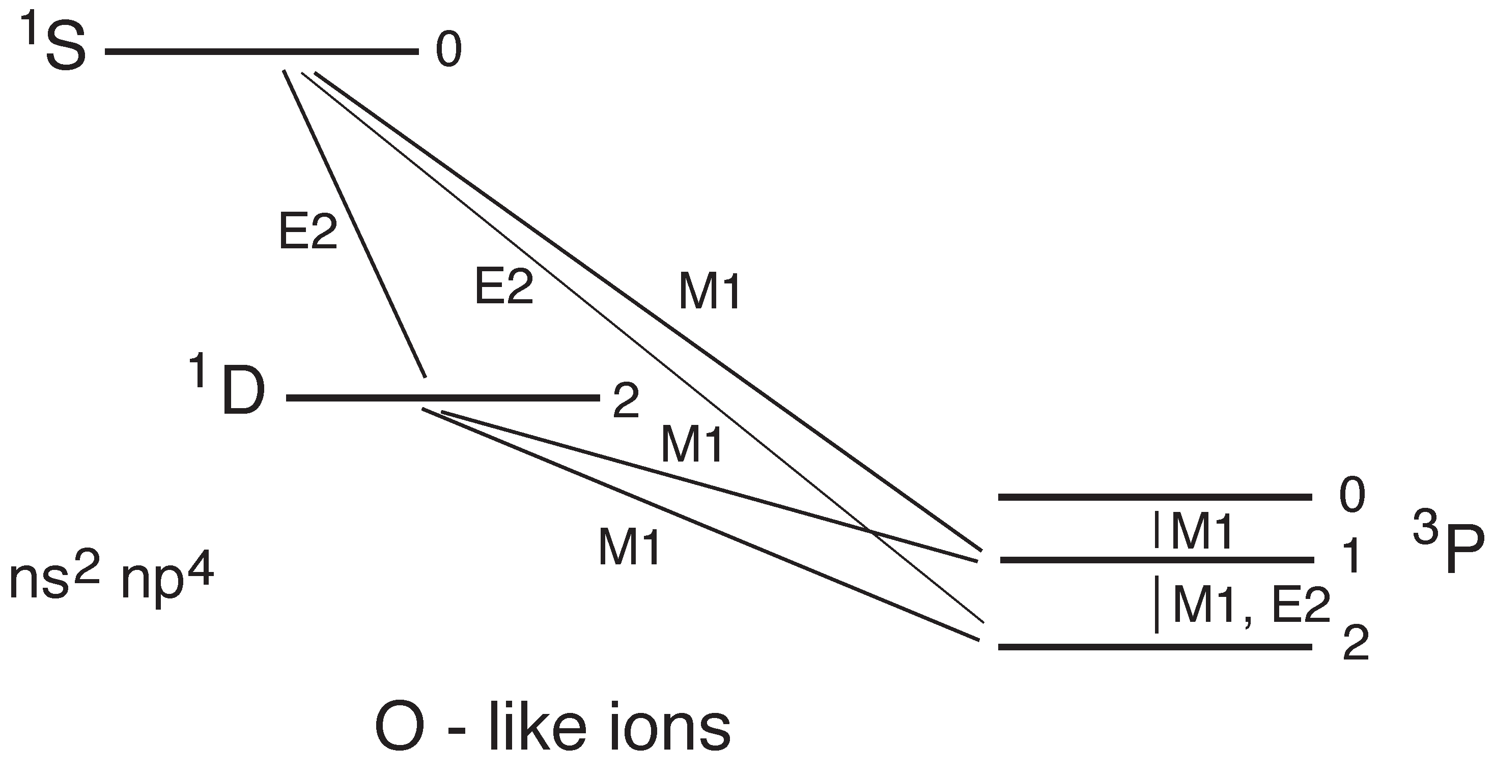
In C-, N- and O-like ions, the ground configuration comprises levels of several multiplicities. Hence the lowest levels of the term systems do not interconnect by spin-changing intercombination transitions, but only by -forbidden transitions that preserve parity. Incidentally, these transitions provide a large fraction of the so-called nebular lines (associated with the mislabeled “planetary nebulae” [63,64,65,66,67,68]).
C-, N-, and O-like ions each feature five fine structure levels in the ground configuration, incidentally distributed over three terms (see Figure 5, Figure 6 and Figure 7). In the C- and O-like systems, the S level has a decay branch that is purely , and that dominates the S level decay in the spectra N II, O III, and F IV. Early on, the lifetime predictions for this level are scattered by factors of 2 to 3. Lifetime measurements at a heavy-ion storage ring have reduced the uncertainty to 2 to 5% in most cases [10,69,70,71]. The D level decays to the P levels are predominantly transitions. In fact, their line ratio is independent of the level lifetime, because the upper level is the same. What interest might be in such a case beyond the lifetime measurement (not yet achieved)? These lines of N II (incidentally bracketing the H line in the H I spectrum) and O III are quite prominent in astrophysical sources, whether planetary nebulae or rather distant galaxies. If one knows their line ratio, one can better treat the spectral analysis of nearby other lines. Theory predicts a line ratio near the value of 3. Actually, theory predicts the transition rate of each line, and the sum would be the inverse of the level lifetime. However, the ratio of most theoretical results scatters by roughly 1%, while the sum of the same results varies by some 10%. This is suspicious. In the older work, Racah algebra was usually applied to levels with an implicitly assumed single-configuration composition. Storey and Zeippen [72] have obtained slightly different line ratios from a more complex level composition. It would be good to have good experimental numbers on the line ratio, and an interesting approach towards this goal, the evaluation of astrophysical data (suffering from many technical limitations and observational problems) seem to yield results that are in better agreement with the newer computational results (see discussion and references in [1]).
N-like ions feature a half-filled valence shell with -forbidden transitions only (see Figure 6). The level structure differs from those of C- and O-like ions in particular by the large gap between the 2p ground configuration ground term S and the P, D terms. This difference is being exploited in astrophysics, because various line ratios depend on temperature and density, and the N-like ions are more suitable as temperature diagnostics while the smaller term differences in C- and O-like ions are preferred for density diagnostics [68].
O-like ions have a ground configuration rather similar to that of C-like ions, but the level sequence in the P term is inverted (Figure 7). The -forbidden transitions within the ground term closely correspond to those in the C-like ions.
F-like ions with their more-than-half-filled valence shell have a single ground term like the B-like ions do, but the fine structure level sequence is inverted. Thus most of the above notes on B-like ions apply correspondingly to F-like ions and their transitions.
5.3. Ne-like Ions
Ne-like ions (ground configuration 2s2p) have 35 excited levels in the two subshells that arise from either a 2s or a 2p electron being promoted to the shell. There are many interesting details and different level lifetimes. However, for a discussion of long-lived excited levels, it is sufficient to look at the four 2s2p3s levels P and P. The two levels can decay to the ground level by resonance and intercombination decay, respectively—similarly to the two-electron ions of the He isoelectronic sequence. The level decays via an transition to the ground (as in a He-like ion; measured in Fe XVII [73]). The level cannot do the same ( is forbidden), but it can (slowly) decay to the lower level by an fine structure transition, because the fine structure level sequence is inverted. This is all there is in terms of long-lived levels in Ne-like ions, especially at low Z, if the ion is left unperturbed. However, what perturbation could show up in the lifetime pattern? In the technical plasma of a fusion experiment, magnetic fields are used to confine the hot plasma; there are (weak) magnetic fields at the surface of the Sun, and there is a reasonably strong magnetic field that compresses and guides the electron beam of an electron beam ion trap. Such a magnetic field spoils the spherical symmetry of the atom’s Coulomb field, and thus it may modify the transition rates. The effect is rather small and hardly noticeable on a moderate or high transition rate. However, a rate that used to be zero and now amounts to something means that a spectral line might appear where there was none before. What used to be a strict rule against transitions no longer applies to a (slightly) distorted set of wave functions. The effect (dubbed “magnetically induced transitions”—MIT) has been seen and even measured in Ne-like Fe ions in the Livermore electron beam ion trap [74]. Meanwhile, other transitions in other ions have been suggested as a B-field diagnostic for the solar corona, and the first steps of the necessary systematics have been investigated experimentally and theoretically by the Shanghai EBIT group and their collaborators [75,76].
5.4. Mg- through Cl-Like Ions
The structure and spectra of low-lying levels (principal quantum number n = 3) in Mg- through Cl-like ions are similar to those of n = 2 states in Be- through F-like ions, with long-lived levels mostly associated with intercombination transitions and transitions [77,78,79]. The many electrons in the open valence shell complicate the atomic structure as well as the theoretical attempts to calculate the atomic system. For example, see Figure 5, in C-like ions there is a 2s2pS level. In the somewhat analogous case of Si-like ions, there is a 3s3p S level with spin-changing intercombination decays to the ground term. Figure 5 is much simplified as it leaves out the other 2s2p levels, of which the analogous 3s3p levels appear in the term system of Si-like ions. They are important for the lifetime of the S level, which mixes not with just one other level of similar total angular momentum J, but with two: P and D. This complexity has taken years to find out and compute properly. Not enough, there are 3s3p3d levels of the same parity, and some of them are long lived; for example, the 3s3p3d F levels [80].
Essentially, the 3d levels add a significant complication that for long-lived levels begins inconspicuously in Al-like ions and becomes drastic in ions with a few more electrons in the shell. Above, the B-like ions have been described as the lightest ions with fine structure splitting in the ground term and thus with -forbidden transitions between the fine structure levels. Because the lifetime of the upper fine structure level is so much longer than that of all other levels that are notably populated in typical processes, the 2s2p P level lifetime can be measured with an uncertainty well below 1%. Alas, the decay curves of the 3s3p P level in Al-like ions, from experiments at an electrostatic ion trap (fed by an ECR ion source), at a heavy-ion storage ring (fed by a tandem accelerator), or in an EBIT (at Livermore and Heidelberg [81,82,83]), yielded lifetime results that differed by more than the (mostly statistical) error estimates, which were not as tight as those obtained for the B-like ions [84]. Eventually, an interloper was found: the 3s3p3d F level stands out because of its high total angular momentum. The dominant decay branch of that level is by transition to the 3s3p3d F level; this transition has a very low transition energy and consequently a low rate. Calculations put the level F level lifetime close to that of the 3s3p P level (see [79]), though with a slightly different isoelectronic trend. Eventually the cascade (via the 3s3p P levels and subsequent spin-changing intercombination transitions) reaches the ground term levels. Thus, the 3s3p3d F level contributes to the decay curve of the 3s3p P level, where it is difficult to disentangle the two components of almost similar lifetime. However, the higher-lying level may safely be expected to be less populated than the 3s3p P level, so that the cascade is weaker than the primary decay.
Similarly, long-lived 3d levels are present in the isoelectronic sequences of Si I and beyond (see example in Figure 8). The levels typically are long-lived for the same reasons as described above: their high total angular momentum precludes a 3p-3d transition and thus leaves open only a higher-multipole order decay, most often an transition to another 3d level of the same term, then followed by a 3p–3d intercombination transition. In several cases, the decays of the long-lived levels should be observable in the solar corona (where the density is low enough not to quench the levels by collisions), but there are so many lines in the solar EUV spectrum that many of them have not yet been identified. In contrast, their cascade contributions have clearly been seen in low-level decay curves obtained (through filters for the visible light of the transitions) at the Heidelberg heavy-ion storage ring TSR [79], without any spectroscopic means to observe and resolve the EUV transitions directly.
In S- and Cl-like ions there are so many long-lived 3d levels that their superposed decay curves (if not spectrally resolved) should overburden multi-exponential analyses even before the cascades reach the ground configuration and replenish their levels. Not quite as long-lived are the 3d levels, with a total angular momentum below the maximum and lifetimes in the nanosecond range owing to their intercombination decays. (Fully allowed transitions in highly charged ions usually relate to levels with lifetimes of many picoseconds).
Older computations often do not include the high-J levels of present interest, but some newer ones do; for example, those by Wang et al. [85]. Let me refer to their results on ions of Fe, with quantitative information on differential metastability in low-lying terms of S-like ions. In the term system Fe XI, the ground configuration is 3s3p, with five levels of lifetimes from 1 ms to several seconds and -forbidden decay channels only. There are four 3s 3p levels with lifetimes shorter than 1 ns, all having decay channels; as well as some 38 levels of the 3s 3p 3d configuration, which fall into three groups of level lifetimes: some 21 levels have lifetimes in the picosecond to subnanosecond range, some 11 levels have lifetimes of a few nanoseconds, and six levels have lifetimes in the millisecond range. These latter levels are D, F, G, G, G, and again F (with a different coupling). Evidently, these long-lived levels feature a high total angular momentum quantum number that results in their strongest decay channel being an transition in the same term. Hardly any of these long-lived levels are represented in the NIST online database [3] because they do not directly contribute to the classical EUV spectra; moreover, they might have been quenched by collisions in most terrestrial light sources. Is there any evidence that they are more than a computational artifact? Delayed beam-foil spectra [86] show a time variation that clearly points to the intercombination decays of the medium-long lifetime levels and to the existence of the long-lived levels. At the heavy-ion storage ring, the cascade tails tell of the long-lived levels [78,79], but spectrally resolved lifetime measurements of all the cascade transitions are technically a long way off. Beam-foil spectroscopy would in principle be suitable for the study of the medium-long lifetime levels, but ion trapping techniques and ultra-high vacuum are necessary for the investigation of the long-lived ones.
The ions in this section have been studied for lifetimes mostly on -forbidden transitions, using electrostatic ion traps, a heavy-ion storage ring, and EBITs. One aim was the provision of results on several elements and ions in a given isoelectronic sequence, so that, by inter-comparison under the guidance of known systematic trends, cross-checks should become feasible and help with assessing errors. As has been demonstrated elsewhere [79], databases have inconsistencies, computational results in some cases come close to each other and scatter considerably in others (by up 40%, some clearly beyond the uncertainties of the measurements), and experimental results scatter somewhat, suggesting that the experiments ought to be refined as well. Last, but not least, in low charge states the transition energies are so low that the transition rates must also be very low (and the level lifetimes too long for presently available measurement techniques). For example, in astrophysics some singly charged ions give rise to (-forbidden) line ratios that are sensitive to the low densities in planetary nebulae. One of these is S II (P-like), involving level lifetimes on the order of 1 h [87]. With elements of the Fe group, highly charged ions of the P I isoelectronic sequence feature millisecond lifetimes and have been the subject of experiments [79]. For elements as heavy as Kr () most computations converge to a narrow range of results, but for the ions of the iron group, the trends of the predictions diverge towards lower Z, prohibiting any meaningful evaluation towards the lowest charge states [79]. A very recently developed new technique, “weighing” ions in an ion trap, might permit direct measurements of some very long key lifetimes in the near future (see below).
5.5. Ar-like Ions
The ground configuration of Ar-like atomic systems (neglecting the core electrons) is 3s 3p, which forms a single S level. The first excited configuration 3s 3p 3d features 12 levels with more than 12 decay channels, not all of which are drawn in Figure 9 (which approximates the level structure of Fe IX), in order to avoid visual clutter. For example, Figure 9 shows an decay of the F level to the F level, but this is only a representative for the three such decays to all three J levels of the F term. There are also transitions (not drawn) within each term. There are three resonance () transitions with notably different upper-level lifetimes (see the transition rates in the “lines” form offered by the NIST ASD online database [3]). In beam-foil spectroscopy, only the two faster decays of the three have been observed [88], whereas the signal-to-noise ratio of the decay of the longest-lived resonance level was not good enough to detect the line. In contrast, all three decays have been seen in EBIT spectra and in the solar corona. In the latter two settings, the density is so low that the radiative decay is not overwhelmed by collisional de-excitation.
In Fe IX, the lowest excited term is 3s3p3d P with three fine structure levels of total angular momentum values . There is no single-photon transition that would connect the level with the ground state. The level can decay by an spin-changing (intercombination) transition (at a wavelength of 24.4909 nm [89]) to ground, with a predicted transition rate near 10 s [90]. The level decays by a magnetic quadrupole () transition of about 70 s [90], at a wavelength of 24.1739 nm [89]. This level decay has very recently been observed at the Livermore SuperEBIT [91] and at the Shanghai EBIT [75].
In a moderate (or higher) density environment, the intercombination line should appear brighter than the transition by several orders of magnitude (the transition rate is about five orders of magnitude higher). However, in a low-density environment the collisional population of the levels plays a dominant role, and the levels may be not so differently populated. In the (very-low-density) solar corona, a line ratio of about two has been observed, and collisional-radiative (CR) models aiming at a reliable density diagnostic for the solar corona [92] are compatible with such a value. However, the modeling assumptions are contested by the various authors. Could the (about 13 ms) lifetime of the level be measured? Maybe—a level lifetime measurement with sufficient spectral resolution in the EUV spectral range is not quite impossible. In the same 3s3p3d shell there are six long-lived levels with (in Fe IX) lifetimes in the range of several or many milliseconds. For three of these, lifetime measurements at a heavy-ion storage ring have yielded results with error bars from 5 to 10%. The results agree with theory within 50 to 80%, which is not satisfying, neither for the measurement precision nor for the accuracy need for reliable information (see [44] for references).
5.6. K-like Ions
K-like ions feature a single electron outside closed shells. This might seem like a relative of the alkali atoms that have been studied by theory and experiment with high accuracy. However, this is not an s electron with an s-p resonance transition, but a 3d electron, and thus the ground term (disregarding in the notation the 3p S closed-shell core) is D, and it has fine structure. In the astrophysically useful spectrum Fe VIII, the fine structure splitting gives rise to an transition in the infrared, and the low transition energy results in a predicted level lifetime of 14 s [93]. A long-lived level, indeed. By the way, the NIST ASD online database lists the levels of the 3p 4f F and 3p 4f F terms, levels that can decay to the 3p 3d D levels (by transition in the EUV), but neither 3p 4s S nor 3p 4d D, which cannot decay this way. Apparently there are no sufficiently good wavelength data (on ground state transitions in the EUV, or of 4s-4p-4d-4f transitions; 4p-4f transition wavelengths from theory [94] are used) that would merit an inclusion in the database and yield proper 4s and 4d level energies. The 4s level that only has -forbidden decay channels should be relatively long lived—Czyzak and Krueger [94] calculate a value of about 2.3 μs, whereas the other levels (all dominated by decays) have lifetimes around 1 ns.
5.7. Ni-like Ions
In many multi-electron ions there are peculiarly long-lived levels, see the Ti-like ions mentioned below. This discussion picks out prominent examples.
Ni-like ions do not have noble gas electron configurations, but the closed 3d shell of the ground state resembles that of a noble gas. If one of the 3d electrons is excited, the core and the excited electron can combine to a variety of interesting levels. For example, a 3d4s D level cannot decay to the ground state by an , , or transition, for total angular momentum or parity reasons. While the other 3d4s D levels have and/or decay branches, an transition is of the lowest multipole order required for the decay of the D level. Such cases of magnetic octupole transitions were first recognized at the Livermore electron beam ion trap when studying Th and U [95]. A theoretical analysis of such decays in Ni-like ions (and corresponding decays in Pd-like ions) was undertaken a few years later by Biémont [96]. The first measurement of the decay rate (and the long lifetime) of the 3d4s D level was pursued at the Livermore EBIT on ions of Xe, Cs, and Ba [97,98]. Interestingly, the lifetime prediction from a first-order treatment by a friendly theorist agreed reasonably well with the observed lifetime, while a second-order treatment, expected to be more precise, came out in poorer agreement. However, this is not a place to chide theory because the experiment was also still finding its way. The Livermore group noticed that an experiment with specific isotopes was warranted [99], and, indeed, the lifetime result showed a clear influence of the hyperfine structure on the level lifetime for odd isotopes versus even ones (the latter without hyperfine structure). The hyperfine interaction influence on the level lifetime was corroborated by theoretical studies on various isotopes [100,101,102]. This is a problem/option mostly for heavy elements with their many isotopes—isotopically enriched samples for experimental work can be costly.
The 3d4s D level in Ni-like ions plays a special role by virtue of its long lifetime, even without an accurate quantification of the lifetime. It is customary to use collisional-radiative modeling in the prediction of the spectra of laser-produced and other plasmas that involve highly charged ions. Seeing specific lines identifies the charge states reached and thus indicates temperature. Repeatedly it has been noted that such predictions may err when metastable states are left out of the model. The particular process of “stepping-stone” (or “ladder”, or “indirect”) ionization has been mentioned in work at electron beam ion traps, because there the electron beam energy is rather well-defined so that individual ionization steps involving metastable levels can be monitored [103,104,105,106]. For example, in Xe XXVII the excitation energy of the metastable level (about 600 eV) is well below the ionization potential of about 1.5 keV. Consequently, an ion excited to the metastable level needs only another collision of 900 eV or more to become ionized (and thus turn into a Co-like ion), effectively lowering the ionization threshold and thus shifting the charge state balance in the plasma. In EBIT spectra the appearance of lines of Co-like ions at the lower threshold, helped by the metastable level, instead of only when the electron beam energy exceeds the standard value of the ionization potential, is easily observed [103].
5.8. Hyperfine Structure Again
As already mentioned above with an example of hyperfine mixing in He-like ions, the phenomenon of hyperfine interaction may affect ions of many elements. Of particular interest (for their simplicity) appear to have been two-electron spectra (He-, Be-, Mg-, Zn-like ions), for which theoretical treatments are available (among numerous others, [26,107,108,109,110,111,112,113,114,115,116]).
Actual lifetime measurements of ions that are sensitive to hyperfine structure are much more rare (but there are some, involving not very long-lived levels in ions of, say, F or Al). Brage et al. [117] have interpreted the line ratios in a time-integrated astrophysical observation of Be-like N IV in terms of a hyperfine-induced transition rate and a computed level lifetime on the order of 40 min. Schippers et al. [118,119] have measured the hyperfine-shortened lifetime of the 2s2p P level in Be-like S and Ti ions in a heavy-ion storage ring; the results are at some variance with predictions [108]. Träbert et al. have employed the same heavy-ion storage ring to obtain , and hyperfine-induced decay rates in Mg-like ions of Co and Cu (with corresponding measurements on a Ni isotope without hyperfine structure) [120].
5.9. Assorted Samples
The examples in this section so far are so singular that they evade an entry into systematization, but that may change with future experiments.
The metastable levels that provide stepping stones for ionization may also act as “population traps” that modify otherwise simple cascade chains. In one such case, a particular decay in Pm-like ions has been expected by some to be possibly bright, but was not actually seen; for this level system, Kobayashi and colleagues have since found in their collisional-radiative models that such a population trap hindered the upper level of the decay of interest from becoming prominently populated [121,122].
A relative to the Ni-like ions discussed above are Pd-like ions, as has been recognized by Biémont [96]. The Livermore experiments on Ni-like ions aimed at the long-lived 3d4s D level and its decay; the decay curve observation started at the interruption of the excitation process by suddenly lowering the electron beam energy below the excitation threshold. In contrast, Kimura et al. [123] maintained their EBIT at constant settings and built up a steady-state reservoir of ions in the metastable 4d5s level. They used these ions as a starting level for (fast) pulsed laser excitation (pulse length 10 ns) to the moderately-long lived 4d5s level (s), the decay of which (toward the ground level) was observed for a lifetime measurement. Here, the starting time for the decay signal is given by the laser that selectively pumps the fine structure level of interest which is, however, also populated continually by the working EBIT.
A long-lived level acting as a population trap is also the likely reason for the prominence of a spectral line in the spectrum of Ti-like ions [124] that has been observed in many EBIT experiments (for references, especially on—mostly theoretical—level lifetimes, see [125]). This does not need to be the upper level of the fine structure transition so unexpectedly prominently observed, it could as well be an intermediate level that feeds the transition. In an EBIT experiment without optical detection, a long-lived level was detected in a Ti-like ion, but without further specification [126]. The original intention of the search that brought up the Ti-like ion transition [124] was to find a visible spectrum line in highly charged uranium that would permit highly resolved optical observations in a hot plasma (using a Fabry-Pérot interferometer that depends on the light transmission through lenses), and by the Doppler width revealing the plasma temperature [127]. By chance, the wavelength of this transition does not vary very much for a rather wide section of the isoelectronic sequence, so that many heavy trace elements in (contaminants of) a plasma can be exploited with this diagnostic tool.
For various technical reasons, the accuracy of atomic lifetime measurements is (presently) highest for level lifetimes on the order of 10 ms. This is not a matter of clock precision, but of ion storage and signal detectors. Ions in low charge states have been stored for days by now, and singly charged ions forever (almost). However, a long-lived level in an ion de-excites only once, whereas the detector noise accumulates continually, even if the detector is being cooled in order to reduce the thermal noise. Thus, optical detection is impractical for the measurement of very long level lifetimes (see discussion and references in [87]). An interesting alternative has been developed at the Max Planck Institute for Nuclear Physics at Heidelberg [128,129]. Their ultra-sensitive Penning ion trap can detect the mass difference between a single ion in the ground state and an excited one. This technique might be developed into a tool for the measurement of long atomic lifetimes, by detecting whether the stored ion is in a metastable state or not, and freshly exciting it, if it is found in the ground state. The statistics of the on/off signal yield the radiative lifetime, a procedure that has proven its validity decades ago with much shorter atomic lifetimes. (Such an approach for trapped highly charged ions has also been modeled electronically at the Shanghai EBIT laboratory [130]).
Long-lived level ions are used for optical clocks. It is not necessary to actually know the level lifetime precisely, but the longer it is, the narrower the line width and the uncertainty of the transition frequency. An example, the transition in Yb II (Yb) [2], has already been mentioned in the introduction. Frequently transitions in highly charged ions are mentioned (see [131]), but the search aims at low transition rates and therefore seeks out low transition energies. In highly charged ions, the fine structure intervals may become rather large, and hyperfine structure intervals should be smaller. Incidental low transition energies in the chance proximity of levels changing sequence are another option, and the search is on to find small transition intervals that are shielded by atomic structure against level shifts caused by external fields. Another transition discussed is the 3s3p P level decay in Al, which is enabled by the hyperfine interaction; here, the investigation of possible error sources has already progressed to the suggestion to add a second slow transition with different systematic errors, in this case, the 3s3p P level decay via radiation [132]. The option of laser cooling a (wanted) contaminant in order to sympathetically cool the actual trapped ions that form on the clock has already been mentioned—that part of the experiment has already been achieved at Heidelberg. These optical clocks are not solely a goal of their own, but attempting to increase the detail “we” can detect and measure (see the extensive discussion of physical effects involved in the development of the next generations of optical clocks, practical atomic systems, and candidate research topics in [62]). Among the hoped-for applications are the idea to measure the variability of “fundamental” units with time in the universe, a better understanding of the ocean of gravitational waves, the composition of dark matter or of pervasive oscillations in the cosmos that produce similar phenomena, and so on.
6. Computations
The first electronic atomic structure computations (around 1950) used a Numerical Coulomb Approximation, that is, the basic assumption was that of a single valence electron outside of a rump of all other electrons in their ground state, and thus a problem close to an effectively one-electron system without any notable long-lived levels. In the 1950s and 1960s, the structure of the He atom was pursued computationally, but largely without an eye on -forbidden transition rates. In the 1970s, various codes saw the light that addressed multi-electron atomic systems. However, by todays standards, those computers were as big as a large office, yet with the computing power of a modern toy pocket calculator (but much more awkward to handle). The program developers were clever, nevertheless (not much human evolution in such a short time span). When (much later) I asked about specific transitions not usually published, one of the co-developers of such an atomic structure code told me (in the 1990s) that their early programs did contain “buttons” to include , , and further higher-order transitions, as well as higher orders of interaction parameters, but that for limits of computer capacity in the olden days the buttons had not been activated. Maybe some of them had not been tested either—I never got to see any results from “just operating that button”. In the 1980s and 1990s, when several groups pursued the measurement of higher-multipole order transition rates, it was still useful to ’talk to your friendly theorist’, and the world of -forbidden transition rates would open up. Interesting spectral lines popped up in previously empty (to prediction) spectral sections, and long-lifetime predictions corroborated the experimental evidence of delayed emission seen in beam-foil spectra.
When in the 1990s I asked a prominent theoretician whether I should bother to measure certain such -forbidden transition rates, I was told that with such a good state of theory, it was probably not worth it. The outcome of some measurements proved otherwise (see two of the various examples below). A key case is the transitions between the fine structure levels of a given term. Theory has long since identified that this transition rate depends on Racah algebra (geometry) and on the transition energy [59]. However, theory is challenged with the accurate determination of the transition energy, and often replaces the computed transition energy value with a spectroscopically measured one. A second problem lies in the simplification of assuming a single configuration describing a level, which in many cases is good enough, but not in all, requiring a correction to the factor obtained by single configuration Racah algebra. Modern computations address this problem, but would benefit from tests by specific lifetime measurements.
My most striking sample case is demonstrated in predictions and measurements on Fe XIV (Al-like) and Fe X (Cl-like) [82], which relate to prominent lines in the solar corona that can be observed during eclipses. Most of the published theoretical predictions of the transition rate in the ground term agree with each other within a narrow interval, while a few others deviate by up to some 30%. The worst deviations represented pure computational theory, without the aforementioned correction for the experimental transition energy. One predictive data set was correct for the one, but not for the other ion. What to say in light of this about the predictive power of computation/theory? The experiment had a much smaller scatter, but it also suffered a learning curve related to the purity of the ultrahigh vacuum system and to cascade repopulation from initially overlooked high-lying levels of a long lifetime [36,43]. One has to recognize them to include them in the computation and in the data evaluation.
7. Discussion
Long-lived levels in highly charged ions are not peculiar, but they tell about atomic structure details in a way that differs from the common resonance or diagram lines that are enabled by the electric dipole operator. A level that decays via radiation often is short-lived, which may be difficult to measure precisely for reasons of time resolution. If the level lifetime is longer, time resolution should not be a problem, but the reduction in systematic error may be challenging, because the density of the light source environment may cause notable competition by collisions to the radiative decays. Is the photon similar to the photon? I assume that this is the case. Emission and absorption are described by a series expansion of the radiation field, but that means the coupling of a standard photon to a structured atomic system. Nevertheless, recent research has been looking into light fields to which angular momentum has been ascribed. Concerning long-lived levels in highly charged ions, cosmologists and fundamental physicists are becoming aware of new capabilities. For example, some four decades ago the Eötvös concept of searching for a fifth force by a torsion balance was explored. Among the latest suggestions in that field is the application of long-lived levels in highly charged ions to the search for a Fifth Force [133]. The field of long-lived levels in highly charged ions is alive.
Funding
This research received no external funding.
Data Availability Statement
Most of the data presented in this study are openly available in the NIST ASD online database at https://www.nist.gov/pml/atomic-spectra-database (accessed on 3 December 2023).
Conflicts of Interest
The author declares no conflicts of interest.
References
- Träbert, E. On atomic lifetimes and environmental density. Atoms 2022, 10, 114. [Google Scholar] [CrossRef]
- Lange, R.; Peshkov, A.A.; Huntemann, N.; Tamm, C.; Surzhykov, A.; Peik, E. Lifetime of the 2F7/2 level in Yb+ for spontaneous emission of electric octupole radiation. Phys. Rev. Lett. 2021, 127, 213001. [Google Scholar] [CrossRef]
- Kramida, A.; Ralchenko, Y.; Reader, J.; NIST ASD Team. NIST Atomic Spectra Database; Version 5.7.1; National Institute of Standards and Technology: Gaithersburg, MD, USA, 2019. Available online: https://physics.nist.gov/asd (accessed on 1 June 2021).
- Bertschinger, G.; Schmid, H.; von Buttlar, H. Herkunft des Nachleuchtens in einer gepulsten Argonentladung (Origin of the afterglow in a pulsed argon discharge). Z. Phys. A 1974, 268, 129–132. (In German) [Google Scholar] [CrossRef]
- Träbert, E.; Schmid, H.; von Buttlar, H. VUV-Nachleuchten einer gepulsten Koronaentladung in reinem Argon (VUV afterglow of a pulsed corona discharge in pure argon). Z. Phys. A 1975, 274, 27–32. (In German) [Google Scholar] [CrossRef]
- Laporte, O. Die Struktur des Eisenspektrums. Z. Phys. 1924, 23, 135–175. [Google Scholar] [CrossRef]
- Martin, W.C.; Wiese, W.L. Atomic Spectroscopy. Available online: http://sed.nist.gov/Pubs/AtSpec/total.html (accessed on 1 December 2023).
- Martin, W.C.; Wiese, W.L.; Kramida, A. Atomic Spectroscopy. In Springer Handbook of Atomic, Molecular, and Optical Physics, 2nd ed.; Drake, G.W.F., Ed.; Chapter 11; Springer Nature: Cham, Switzerland, 2023; pp. 177–197. [Google Scholar]
- Drake, G.W.F. (Ed.) Springer Handbook of Atomic, Molecular, and Optical Physics, 2nd ed.; Springer Nature: Cham, Switzerland, 2023. [Google Scholar]
- Träbert, E.; Saathoff, G.; Wolf, A. N II electric quadrupole transition rate measured at a heavy-ion storage ring. Phys. Scr. 2005, 72, 35–37. [Google Scholar] [CrossRef]
- Hylleraas, E.A. Über den Grundterm der Zweielektronenprobleme von H−, He, Li+, Be++ usw. Z. Phys. 1930, 65, 209–225. (In German) [Google Scholar] [CrossRef]
- White, H.E.; Eliason, A.Y. Relative intensity tables for spectrum lines. Phys. Rev. 1933, 44, 753–756. [Google Scholar] [CrossRef]
- Chen, H.; Beiersdorfer, P.; Gu, M.-F.; Heeter, L.A.; Lepson, J.K.; Liedahl, D.A.; Naranjo-Rivera, K.L.; Träbert, E. Experimental and theoretical evaluation of density-sensitive N VI, Ar XIV, and Fe XXII line ratios. Astrophys. J. 2004, 611, 598–604. [Google Scholar] [CrossRef]
- Jitrik, O.; Bunge, C.F. Transition probabilities for hydrogen-like atoms. J. Phys. Chem. Ref. Data 2004, 33, 1059–1070. [Google Scholar] [CrossRef]
- Lamb, W.E.; Retherford, R.C. Fine Structure of the Hydrogen Atom by a Microwave Method. Phys. Rev. 1947, 72, 241–243. [Google Scholar] [CrossRef]
- Pritchard, J.R.; Loeb, A. 21 cm cosmology in the 21st century. Rep. Prog. Phys. 2012, 75, 086901. [Google Scholar] [CrossRef]
- Hannen, V.; Vollbrecht, J.; Andelkovic, Z.; Brandau, C.; Dax, A.; Geithner, W.; Geppert, C.; Gorges, C.; Hammen, M.; Kaufmann, S.; et al. Lifetimes and g-factors of the HFS states in H-like and Li-like bismuth. J. Phys. B At. Mol. Opt. Phys. 2019, 52, 085003. [Google Scholar] [CrossRef]
- Drake, G.W.F. Spontaneous two-photon decay rates in hydrogenlike and heliumlike ions. Phys. Rev. A 1986, 34, 2871–2880. [Google Scholar] [CrossRef] [PubMed]
- Johnson, W.R.; Plante, D.R.; Sapirstein, J. Relativistic calculations of transition amplitudes in the helium isoelectronic sequence. Adv. At. Mol. Opt. Phys. 1995, 35, 255–329. [Google Scholar]
- Träbert, E.; Pinnington, E.H. Spectroscopy of ions using fast beams and ion traps. In Springer Handbook of Atomic, Molecular, and Optical Physics, 2nd ed.; Drake, G.W.F., Ed.; Chapter 19; Springer Nature: Cham, Switzerland, 2023; pp. 269–281. [Google Scholar]
- Drake, G.W.F. Theoretical energies for the n = 1 and 2 states of the helium isooelectronic sequence up to Z = 100. Can. J. Phys. 1988, 66, 586–611. [Google Scholar] [CrossRef]
- Marrs, R.E.; Beiersdorfer, P.; Schneider, D.H. The electron beam ion trap. Phys. Today 1994, 47, 27–34. [Google Scholar] [CrossRef]
- Beiersdorfer, P. A “brief" history of spectroscopy on EBIT. Can. J. Phys. 2008, 86, 1–10. [Google Scholar] [CrossRef]
- Birkett, B.B.; Briand, J.-P.; Charles, P.; Dietrich, D.D.; Finlayson, K.; Indelicato, P.; Liesen, D.; Simionovici, A. Hyperfine quenching and measurement of the 2 3P0—2 3P1 fine-structure splitting in heliumlike silver (Ag45+). Phys. Rev. A 1993, 47, R2454–R2457. [Google Scholar] [CrossRef]
- Marrus, R.W.; Schmieder, R.W. Observation of the magnetic-quadrupole decay (2 3P2 → 1 1S0) of heliumlike Ar XVII and lifetime of the 2 3P2 state. Phys. Rev. Lett. 1979, 25, 1689–1691. [Google Scholar] [CrossRef]
- Indelicato, P.; Parente, F.; Marrus, R. Effect of hyperfine structure on the 2 3P1 and the 2 3P0 lifetime in heliumlike ions. Phys. Rev. A 1989, 40, 3505–3514. [Google Scholar] [CrossRef] [PubMed]
- Indelicato, P.; Birkett, B.B.; Briand, J.-P.; Charles, P.; Dietrich, D.D.; Marrus, R.; Simionovici, A. Hyperfine quenching and precision measurement of the 2 3P0 – 2 3P1 fine-structure splitting in heliumlike gadolinium (Gd62+). Phys. Rev. Lett. 1992, 68, 1307–1310. [Google Scholar] [CrossRef] [PubMed]
- Munger, C.T.; Gould, H. Lamb shift in heliumlike uranium (U90+). Phys. Rev. Lett. 1986, 57, 2927–2930. [Google Scholar] [CrossRef]
- Träbert, E. The allure of high total angular momentum levels in multiply-excited ions. Atoms 2019, 7, 103. [Google Scholar] [CrossRef]
- Edlén, B.; Tyrén, F. Atomic energy states of an unusual type. Nature 1939, 3631, 940–941. [Google Scholar] [CrossRef]
- Gabriel, A.H.; Jordan, C. Long wavelength satellites to the He-like ion resonance lines in the laboratory and the sun. Nature 1969, 221, 947–949. [Google Scholar] [CrossRef]
- Gabriel, A.H. Dielectronic satellite spectra for highly-charged helium-like ion lines. Mon. Not. R. Astr. Soc. 1972, 160, 99–119. [Google Scholar] [CrossRef]
- Pietenpol, J.L. Auto-ionization of the (1s2s2p) 4P5/2 level in Li and He−. Phys. Rev. Lett. 1961, 7, 64. [Google Scholar] [CrossRef]
- Beiersdorfer, P.; Bitter, M.; Hey, D.; Reed, K.J. Identification of the 1s2s2p 4P5/2 → 1s22s 2S1/2 magnetic quadrupole inner-shell satellite line in the Ar16+ K-shell X-ray spectrum. Phys. Rev. A 2002, 66, 032504. [Google Scholar] [CrossRef]
- Kaufman, V.; Sugar, J. Forbidden lines in ns2 npk ground configurations and nsnp excited configurations of beryllium through molybdenum atoms and ions. J. Phys. Chem. Ref. Data 1986, 15, 321–426. [Google Scholar] [CrossRef]
- Träbert, E. E1-forbidden transition rates in ions of astrophysical interest. Phys. Scr. T 2014, 89, 114003. [Google Scholar] [CrossRef]
- Church, D.A. Collision measurements and excited-level lifetime measurements on ions stored in Paul, Penning and Kingdon ion traps. Phys. Rep. 1993, 228, 253–358. [Google Scholar] [CrossRef]
- Träbert, E. Atomic lifetime measurements with ion traps of many sizes. Phys. Scr. 2000, 61, 257–286. [Google Scholar] [CrossRef]
- Träbert, E. Precise measurements of long atomic lifetimes using stored ion beams and ion traps. Can. J. Phys. 2002, 80, 1481–1503. [Google Scholar] [CrossRef]
- Mannervik, S. Experimental lifetime studies of metastable levels. Phys. Scr. T 2003, 105, 67–75. [Google Scholar] [CrossRef]
- Träbert, E. Atomic lifetime measurements using electron beam ion traps. Can. J. Phys. 2008, 86, 73–97. [Google Scholar] [CrossRef]
- Träbert, E. Problems with accurate atomic lifetime measurements of multiply charged ions. Phys. Scr. 2009, 79, 068101. [Google Scholar] [CrossRef]
- Träbert, E. In pursuit of high precision atomic lifetime measurements of multiply charged ions. J. Phys. B At. Mol. Opt. Phys. 2010, 43, 074034. [Google Scholar] [CrossRef]
- Träbert, E. Atomic lifetimes of astrophysical interest in ions of Fe. Atoms 2023, 11, 85. [Google Scholar] [CrossRef]
- Träbert, E.; Wolf, A.; Linkemann, J.; Tordoir, X. Measurement of the B+ and Al+ intercombination and Sc12+ forbidden transition rates at a heavy-ion storage ring. J. Phys. B At. Mol. Opt. Phys. 1999, 32, 537–552. [Google Scholar] [CrossRef]
- Doerfert, J.S.; Träbert, E.; Wolf, A.; Schwalm, D.; Uwira, O. Precision measurement of the electric dipole intercombination rate in C2+. Phys. Rev. Lett. 1997, 78, 4355–4358. [Google Scholar] [CrossRef]
- Träbert, E.; Knystautas, E.J.; Saathoff, G.; Wolf, A. EUV intercombination transition rates in Be-like nitrogen and oxygen ions measured at a heavy-ion storage ring. J. Phys. B At. Mol. Opt. Phys. 2005, 38, 2395–2405. [Google Scholar] [CrossRef]
- Träbert, E. Radiative-lifetime measurements on highly-charged ions. In Accelerator-Based Atomic Physics Techniques and Applications; Shafroth, S.M., Austin, J.C., Eds.; American Institute of Physics: Washington, DC, USA, 1997; pp. 567–607. [Google Scholar]
- Träbert, E.; Curtis, L.J. Isoelectronic trends of line strength data in the Li and Be isoelectronic sequences. Phys. Scr. 2006, 74, C46. [Google Scholar] [CrossRef]
- Jönsson, P.; Froese Fischer, C.; Träbert, E. On the status and perspectives of MCDF computations and measurements of transition data in the Be isoelectronic sequence. J. Phys. B At. Mol. Opt. Phys. 1998, 31, 3497–3511. [Google Scholar] [CrossRef]
- Chen, M.H.; Cheng, K.T.; Johnson, W.R. Large-scale relativistic configuration-interaction computation of the 2s2 1S0 – 2s2p 3P1 intercombination transition in C III. Phys. Rev. A 2001, 64, 042507. [Google Scholar] [CrossRef]
- Träbert, E.; Heckmann, P.H.; von Buttlar, H. Beam-foil lifetimes of highly ionized silicon. Z. Phys. A 1977, 281, 333–339. [Google Scholar] [CrossRef]
- Cheng, K.T.; Kim, Y.-K.; Desclaux, J.P. Electric dipole, quadrupole, and magnetic dipole transition probabilities of ions isoelectronic to the first-row atoms, Li through F. At. Data Nucl. Data Tab. 1979, 24, 111–189. [Google Scholar] [CrossRef]
- Träbert, E.; Gwinner, G.; Knystautas, E.J.; Tordoir, X.; Wolf, A. Precise intercombination transition rates in C+ and N2+ ions measured at a heavy-ion storage ring. J. Phys. B At. Mol. Opt. Phys. 1999, 32, L491–L499. [Google Scholar] [CrossRef]
- Curtis, L.J. Lifetime measurements in highly ionised atoms. Phys. Scr. 1984, 8, 77–83. [Google Scholar] [CrossRef]
- Moehs, D.P.; Church, D.A. Magnetic dipole transition rates from measured lifetimes of levels of Be-like and B-like argon ions. Phys. Rev. A 1998, 58, 1111–1114. [Google Scholar] [CrossRef]
- Träbert, E.; Beiersdorfer, P.; Utter, S.B.; Brown, G.V.; Chen, H.; Harris, C.L.; Neill, P.A.; Savin, D.W.; Smith, A.J. Experimental M1 transition rates of coronal lines from Ar X, Ar XIV, and Ar XV. Astrophys. J. 2000, 541, 506–511. [Google Scholar] [CrossRef]
- Lapierre, A.; Crespo López-Urrutia, J.R.; Braun, J.; Brenner, G.; Bruhns, H.; Fischer, D.; González-Martínez, A.J.; Mironov, V.; Osborne, C.J.; Sikler, G.; et al. Lifetime measurement of the Ar XIV 1s22s22p 2P metastable level at the Heidelberg electron-beam ion trap. Phys. Rev. A 2006, 73, 052507. [Google Scholar] [CrossRef]
- Pasternack, S. Transition probabilities of forbidden lines. Astrophys. J. 1940, 92, 129–155. [Google Scholar] [CrossRef]
- Nemouchi, M.; Godefroid, M.R. Irreducible tensor form of the relativistic corrections to the M1 transition operator. J. Phys. B At. Mol. Opt. Phys. 2009, 42, 175002. [Google Scholar] [CrossRef]
- Leopold, T.; King, S.A.; Micke, P.; Bautista-Salvador, A.; Heip, J.C.; Ospelkaus, C.; Crespo López-Urrutia, J.R.; Schmidt, P.O. A cryogenic radio-frequency ion trap for quantum logic spectroscopy of highly charged ions. Rev. Sci. Instrum. 2019, 90, 073201. [Google Scholar] [CrossRef] [PubMed]
- Kozlov, M.G.; Safronova, M.S.; Crespo López-Urrutia, J.R.; Schmidt, P.O. Highly charged ions: Optical clocks and applications in fundamental physics. Rev. Mod. Phys. 2018, 90, 045005. [Google Scholar] [CrossRef]
- Bowen, I.S. The origin of the chief nebular lines. Proc. Astron. Soc. Pac. 1927, 39, 295B. [Google Scholar] [CrossRef]
- Stevenson, A.F. The intensities of certain nebular lines and the mean lives of atoms emitting them. Proc. R. Soc. A 1932, 137, 298–325. [Google Scholar]
- Boyce, J.C.; Menzel, D.H.; Payne, C.H. Forbidden lines in astrophysical sources. Proc. Nat. Acad. Sci. USA 1933, 19, 581–591. [Google Scholar] [CrossRef]
- Bowen, I.S. Forbidden lines. Rev. Mod. Phys. 1936, 8, 55–81. [Google Scholar] [CrossRef]
- Czyzak, S.J.; Krueger, T.K. Forbidden transition probabilities for some P, S, Cl, and A ions. Mon. Not. R. Astron. Soc. 1963, 126, 177–194. [Google Scholar] [CrossRef]
- Czyzak, S.J.; Keyes, C.D.; Aller, L.H. Atomic structure calculations and nebular diagnostics. Astroph. J. Suppl. 1986, 61, 159–175. [Google Scholar] [CrossRef]
- Träbert, E.; Calamai, A.G.; Gillaspy, J.D.; Gwinner, G.; Tordoir, X.; Wolf, A. Intercombination and forbidden transition rates in C- and N-like ions O2+, F3+, and S9+ measured at a heavy-ion storage ring. Phys. Rev. A 2000, 62, 022507. [Google Scholar] [CrossRef]
- Träbert, E.; Wolf, A.; Pinnington, E.H.; Linkemann, J.; Knystautas, E.J.; Curtis, A.; Bhattacharya, N.; Berry, H.G. Heavy-ion storage ring measurement of forbidden transition rates between ground-configuration levels in Si6+ and Si8+ ions. Can. J. Phys. 1998, 76, 899–906. [Google Scholar] [CrossRef]
- Träbert, E.; Grieser, M.; Hoffmann, J.; Krantz, C.; Repnow, R.; Wolf, A. Heavy-ion storage-ring-lifetime measurement of metastable levels in the C-, N-,and O-like ions of Si, P, and S. Phys. Rev. A 2012, 85, 042508. [Google Scholar] [CrossRef]
- Storey, P.J.; Zeippen, C.J. Theoretical values for the [O III] 5007/4959 line-intensity ratio and homologous cases. Mon. Not. R. Astron. Soc. 2000, 312, 813–816. [Google Scholar] [CrossRef]
- Crespo López-Urrutia, J.R.; Beiersdorfer, P. Measurement of the radiative decay rate of the metastable (2s22p3s1/2)(J=2) level in Fe XVII. Astrophys. J. 2010, 721, 576–581. [Google Scholar] [CrossRef]
- Beiersdorfer, P.; Crespo López-Urrutia, J.R.; Träbert, E. Measurement of the radiative decay rate and energy of the metastable (2s22p3s1/2)(J=0) level in Fe XVII. Astrophys. J. 2016, 817, 67. [Google Scholar] [CrossRef]
- Xu, G.; Yan, C.; Lu, Q.; Yang, Y.; Li, W.; Ma, S.; Zhao, Z.; Huang, S.; Song, L.; Si, R.; et al. First laboratory measurement of magnetic-field-induced transition effect in Fe X at different magnetic fields. Astrophys. J. 2022, 937, 48. [Google Scholar] [CrossRef]
- Li, W.; Li, M.; Wang, K.; Brage, T.; Hutton, R.; Landi, E. A theoretical investigation of the magnetic-field-induced transition in Fe X, of importance for measuring magnetic field strengths in the solar corona. Astrophys. J. 2021, 913, 135. [Google Scholar] [CrossRef]
- Träbert, E. Intercombination transition probabilities in two-electron spectra. Phys. Scr. 1990, 41, 675–680. [Google Scholar] [CrossRef]
- Träbert, E.; Hoffmann, J.; Krantz, C.; Wolf, A.; Ishikawa, Y.; Santana, J.A. Atomic lifetime measurements on forbidden transitions of Al-, Si-, P- and S-like ions at a heavy-ion storage ring. J. Phys. B At. Mol. Opt. Phys. 2009, 42, 025002. [Google Scholar] [CrossRef]
- Träbert, E.; Grieser, M.; Krantz, C.; Repnow, R.; Wolf, A.; Diaz, F.J.; Ishikawa, Y.; Santana, J.A. Isoelectronic trends of the E1-forbidden decay rates of Al-, Si-, P-, and S-like ions of Cl, Ti, Mn, Cu, and Ge. J. Phys. B At. Mol. Opt. Phys. 2012, 45, 215003. [Google Scholar] [CrossRef]
- Träbert, E.; Ishikawa, Y.; Santana, J.A.; Del Zanna, G. The 3s23p3d 3Fo term in the Si-like spectrum of Fe (Fe XIII). Can. J. Phys. 2011, 89, 403–412. [Google Scholar] [CrossRef]
- Beiersdorfer, P.; Träbert, E.; Pinnington, E.H. Experimental transition rate of the green coronal line of Fe XIV. Astrophys. J. 2003, 587, 836–840. [Google Scholar] [CrossRef]
- Träbert, E. On the transition rates of the Fe X and Fe XIV coronal lines. Astron. Astrophys. 2004, 415, L39–L42. [Google Scholar] [CrossRef]
- Brenner, G.; Crespo López-Urrutia, J.R.; Harman, Z.; Mokler, P.H.; Ullrich, J. Lifetime determination of the Fe XIV 3s23p 2Po metastable level. Phys. Rev. A 2007, 75, 032504. [Google Scholar] [CrossRef]
- Träbert, E. Differential observations in spectroscopic measurements using electron beam ion traps. J. Phys. B At. Mol. Opt. Phys. 2009, 42, 154019. [Google Scholar] [CrossRef]
- Wang, K.; Song, C.X.; Jönsson, P.; Del Zanna, G.; Schiffmann, S.; Godefroid, M.; Gaigalas, G.; Zhao, X.H.; Si, R.; Chen, C.Y.; et al. Benchmarking atomic data from large-scale multiconfiguration Dirac-Hartree-Fock calculations for astrophysics: S-like ions from Cr IX to Cu XIV. Astrophys. J. Suppl. Ser. 2018, 239, 30. [Google Scholar] [CrossRef]
- Träbert, E. EUV beam-foil spectra of germanium and a blind-spot problem in spectroscopy. Atoms 2023, 11, 45. [Google Scholar] [CrossRef]
- Träbert, E. A laboratory astrophysics problem: The lifetime of very long-lived levels in low-charge ions. Atoms 2020, 8, 21. [Google Scholar] [CrossRef]
- Träbert, E. Experimental checks on calculations for Cl-, S- and P-like ions of the iron group elements. J. Phys. B At. Mol. Opt. Phys. 1996, 29, L217–L224. [Google Scholar] [CrossRef]
- Shirai, T.; Funatake, Y.; Mori, K.; Sugar, J.; Wiese, W.L.; Nakai, Y. Spectral data and Grotrian diagrams for highly ionized iron, Fe VIII-XXVI. J. Phys. Chem. Ref. Data 1990, 19, 127–275. [Google Scholar] [CrossRef]
- Del Zanna, G.; Storey, P.J.; Badnell, N.R.; Mason, H.E. Atomic data for astrophysics: Fe IX. Astron. Astrophys. 2014, 565, A77. [Google Scholar] [CrossRef]
- Träbert, E.; Beiersdorfer, P.; Brown, G.V.; Hell, N.; Lepson, J.K.; Fairchild, A.J.; Hahn, M.; Savin, D.W. Laboratory search for Fe IX solar diagnostic lines using an electron beam ion trap. Atoms 2022, 10, 115. [Google Scholar] [CrossRef]
- Storey, P.J.; Zeippen, C.J. Coronal Fe IX line intensities and electron density diagnostics. Mon. Not. R. Astron. Soc. 2001, 324, L7–L10. [Google Scholar] [CrossRef]
- Biémont, E.; Hansen, J.E. Energy levels and transition probabilities in 3d and 3d9 configurations. Phys. Scr. 1989, 39, 308–313. [Google Scholar] [CrossRef]
- Czyzak, S.J.; Krueger, T.K. On the excited levels of Fe VIII. Astrophys. J. 1966, 144, 381–407. [Google Scholar] [CrossRef]
- Beiersdorfer, P.; Osterheld, A.L.; Scofield, J.; Wargelin, B.; Marrs, R.E. Observation of magnetic octupole decay in atomic spectra. Phys. Rev. Lett. 1991, 67, 2272–2275. [Google Scholar] [CrossRef]
- Biémont, E. Multipole transitions in nickel-like and palladium-like spectra. J. Phys. B At. Mol. Opt. Phys. 1997, 30, 4207–4222. [Google Scholar] [CrossRef]
- Träbert, E.; Beiersdorfer, P.; Brown, G.V.; Terracol, S.; Safronova, U.I. On the metastable level in Ni-like ions. Nucl. Instrum. Meth. Phys. Res. B 2005, 235, 23–27. [Google Scholar] [CrossRef]
- Träbert, E.; Beiersdorfer, P.; Brown, G.V.; Boyce, K.; Kelley, R.L.; Kilbourne, C.A.; Porter, F.S.; Szymkowiak, A. Time-resolved soft-x-ray spectroscopy of a magnetic octupole transition in nickel-like xenon, cesium, and barium ions. Phys. Rev. A 2006, 73, 022508. [Google Scholar] [CrossRef]
- Träbert, E.; Beiersdorfer, P.; Brown, G.V. Observation of hyperfine mixing in measurements of a magnetic octupole decay in isotopically pure nickel-like 129Xe and 132Xe ions. Phys. Rev. Lett. 2007, 98, 263001. [Google Scholar] [CrossRef]
- Yao, K.; Andersson, M.; Brage, T.; Hutton, R.; Jönsson, P.; Zou, Y. MF-dependent lifetimes due to hyperfine induced interference effects. Phys. Rev. Lett. 2006, 97, 183001, Erratum Phys. Rev. Lett. 2007, 98, 269903; Reply Phys. Rev. Lett. 2007, 98, 269304. [Google Scholar] [CrossRef]
- Andersson, M.; Yao, K.; Hutton, R.; Zou, Y.; Chen, C.Y.; Brage, T. Hyperfine-state-dependent lifetimes along the Ni-like isoelectronic sequence. Phys. Rev. A 2008, 77, 042509. [Google Scholar] [CrossRef]
- Du, W.; Andersson, M.; Yao, K.; Brage, T.; Hutton, R.; Zou, Y. Lifetimes of the hyperfine levels of 3d94s 3D3 in high-Z Ni-like ions. J. Phys. B At. Mol. Opt. Phys. 2013, 46, 145001. [Google Scholar] [CrossRef]
- Träbert, E.; Beiersdorfer, P.; Gu, M.F. Spectra of Ni- and Co-like ions of Xe in an electron-beam ion trap. Can. J. Phys. 2008, 86, 467–475. [Google Scholar] [CrossRef]
- Sakoda, J.; Komatsu, A.; Kikuchi, H.; Nakamura, N. Visible spectroscopy of Rh-like ions. Phys. Scr. 2011, 144, 014011. [Google Scholar] [CrossRef]
- Kilbane, D.; Gillaspy, J.D.; Ralchenko, Y.; Reader, J.; O’Sullivan, G. Extreme ultraviolet spectra from N-shell ions of Gd, Dy and W. Phys. Scr. 2013, 156, 014012. [Google Scholar]
- Qiu, M.L.; Zhao, R.F.; Guo, X.L.; Zhao, Z.Z.; Li, W.X.; Du, S.Y.; Xiao, J.; Yao, K.; Chen, C.Y.; Hutton, R.; et al. Investigation of transitions between metastable levels of the first excited configuration of palladium-like tungsten. J. Phys. B At. Mol. Opt. Phys. 2014, 47, 175002. [Google Scholar] [CrossRef]
- Marques, J.P.; Parente, F.; Indelicato, P. Hyperfine quenching of the 1s22s2p 3P0 level in berylliumlike ions. Phys. Rev. A 1993, 47, 929–935. [Google Scholar] [CrossRef]
- Cheng, K.T.; Chen, M.H.; Johnson, W.R. Hyperfine quenching of the 2s2p 3P0 state of berylliumlike ions. Phys. Rev. A 2008, 77, 052504. [Google Scholar] [CrossRef]
- Andersson, M.; Zou, Y.; Hutton, R. Hyperfine-dependent lifetimes in Be-like ions. Phys. Rev. A 2009, 79, 032501. [Google Scholar] [CrossRef]
- Andersson, M.; Hutton, R.; Zou, Y. Hyperfine dependent lifetimes in Neon like ions. J. Phys. Conf. Ser. 2009, 163, 012013. [Google Scholar] [CrossRef]
- Marques, J.P.; Parente, F.; Indelicato, P. Hyperfine quenching of the 1s2 2s2 2p6 3s3p 3P0 level in magnesiumlike ions. At.Data Nucl. Data Tab. 1993, 55, 157–170. [Google Scholar] [CrossRef]
- Kang, H.; Li, J.G.; Dong, C.Z.; Jönsson, P.; Gaigalas, G. Hyperfine quenching of the 3s3p 3P0 level in Mg-like ions. J. Phys. B At. Mol. Opt. Phys. 2009, 42, 195002. [Google Scholar] [CrossRef]
- Kang, H.; Li, J.G.; Dong, C.Z.; Jönsson, P.; Gaigalas, G. THe effect of hyperfine interaction on the lifetime of the 3s3p 3P2 level of Mg-like ions. J. Phys. B At. Mol. Opt. Phys. 2010, 43, 095003. [Google Scholar] [CrossRef]
- Andersson, M.; Zou, Y.; Hutton, R.; Brage, T. Hyperfine dependent lifetimes in Mg-like ions. J. Phys. B At. Mol. Opt. Phys. 2010, 43, 095001. [Google Scholar] [CrossRef]
- Marques, J.P.; Parente, F.; Indelicato, P. Hyperfine quenching of the 4s4p 3P0 level in Zn-like ions. Eur. Phys. J. D 2007, 41, 457–465. [Google Scholar] [CrossRef]
- Andersson, M.; Liu, Z.; Chen, C.Y.; Hutton, R.; Zou, Y. Hyperfine-interaction-dependent 4s4p 3P2 lifetimes in Zn-like ions. Phys. Rev. A 2008, 78, 062505. [Google Scholar] [CrossRef]
- Brage, T.; Judge, P.G.; Proffitt, C.R. Determination of hyperfine-induced transition rates from observations of a planetary nebula. Phys. Rev. Lett. 2002, 89, 281101. [Google Scholar] [CrossRef]
- Schippers, S.; Bernhardt, D.; Müller, A.; Lestinsky, M.; Hahn, M.; Novotný, O.; Savin, D.W.; Grieser, M.; Krantz, C.; Repnow, R.; et al. Storage-ring measurement of the hyperfine-induced 2s2p 3P0 → 2s2 1S0 transition rate in berylliumlike sulfur. Phys. Rev. A 2012, 85, 012513. [Google Scholar] [CrossRef]
- Schippers, S.; Schmidt, E.W.; Bernhardt, D.; Yu, D.; Müller, A.; Lestinsky, M.; Orlov, D.A.; Grieser, M.; Repnow, R.; Wolf, A. Storage-ring measurement of the hyperfine induced 47Ti18+ (2s2p 3P0 → 2s2 1S0) transition rate. Phys. Rev. Lett. 2007, 98, 033001. [Google Scholar] [CrossRef]
- Träbert, E.; Grieser, M.; Hoffmann, J.; Krantz, C.; Reinhardt, S.; Repnow, R.; Wolf, A.; Indelicato, P. M1, M2 and hyperfine-induced decay rates in Mg-like ions of Co, Ni and Cu measured at a heavy-ion storage ring. New J. Phys. 2011, 13, 023017. [Google Scholar] [CrossRef]
- Kobayashi, Y.; Kato, D.; Sakaue, H.A.; Murakami, I.; Nakamura, N. Spectroscopic study of promethiumlike bismuth with an electron-beam ion trap: Search for alkali-metal-like resonance lines. Phys. Rev. A 2014, 89, 010501(R). [Google Scholar] [CrossRef]
- Kobayashi, Y.; Kubota, K.; Omote, K.; Komatsu, A.; Sakoda, J.; Minoshima, M.; Kato, D.; Li, J.; Sakaue, H.A.; Murakami, I.; et al. Extreme ultraviolet and visible spectroscopy of promethiumlike heavy ions. Phys. Rev. A 2015, 92, 022510. [Google Scholar] [CrossRef]
- Kimura, N.; Priti; Kuma, S.; Azuma, T.; Nakamura, N. Electric-quadrupole transition-rate measurement of a highly charged ion in an electron-beam ion trap using pulsed laser excitation from a metastable state. Phys. Rev. A 2023, 107, 022805. [Google Scholar] [CrossRef]
- Feldman, U.; Indelicato, P.; Sugar, J. Magnetic dipole line from U LXXI ground-term levels predicted at 3200 Å. J. Opt. Soc. Am. B 1991, 8, 3–5. [Google Scholar] [CrossRef]
- Biémont, E.; Träbert, E.; Zeippen, C.J. Calculated transition probabilities in highly charged Ti-like ions. J. Phys. B At. Mol. Opt. Phys. 2001, 34, 1941–1951. [Google Scholar] [CrossRef]
- Tu, B.; Yao, K.; Shen, Y.; Yang, Y.; Li, M.C.; Xu, T.H.; Lu, Q.F.; Lu, D.; Wang, X.; Chen, C.Y.; et al. Observation of an extremely-long-lived metastable level in a Ti-like system via an L-shell dielectronic recombination measurement in highly charged 3dn ions of tungsten. Phys. Rev. A 2017, 96, 032705. [Google Scholar] [CrossRef]
- Adler, A.; Meyer, E.S.; Serpa, F.G.; Takacs, E.; Gillaspy, J.D.; Brown, C.M.; Feldman, U. Fabry-Perot spectroscopy of a visible magnetic dipole transition in Ba34+. Nucl. Instrum. Meth. Phys. Res. B 1995, 98, 581–584. [Google Scholar] [CrossRef]
- Schüssler, R.X.; Bekker, H.; Braß, M.; Cakir, H.; Crespo López-Urrutia, J.R.; Door, M.; Filianin, P.; Harman, Z.; Haverkort, M.W.; Huang, W.J.; et al. Detection of metastable electronic states by Penning-trap mass spectrometry. Nature 2020, 581, 42–46. [Google Scholar] [CrossRef] [PubMed]
- Kromer, K.; Lyu, C.; Door, M.; Filianin, P.; Harman, Z.; Herkenhoff, J.; Indelicato, P.; Keitel, C.H.; Lange, D.; Novikov, Y.N.; et al. Observation of a low-lying metastable electronic state in highly charged lead by Penning-trap mass spectrometry. Phys. Rev. Lett. 2023, 131, 223002. [Google Scholar] [CrossRef] [PubMed]
- Tu, B.; Si, R.; Shen, Y.; Wang, J.; Wei, B.; Chen, C.-Y.; Yao, K.; Zou, Y.-M. Experimental access to observing decay from extremely long-lived metastable electronic states via Penning trap spectrometry. Phys. Rev. Res. 2023, 5, 043014. [Google Scholar] [CrossRef]
- Yudin, V.I.; Taichenachev, A.V.; Derevianko, A. Magnetic-dipole transitions in highly charged ions as a basis of ultraprecise optical clocks. Phys. Rev. Lett. 2014, 113, 233003. [Google Scholar] [CrossRef]
- Bohman, M.A.; Porsev, S.G.; Hume, D.B.; Leibrandt, D.R.; Safronova, M.S. Enhancing divalent optical atomic clocks with the 1S0 ↔3P2 transition. Phys. Rev. A 2023, 108, 053120. [Google Scholar] [CrossRef]
- Rehbehn, N.-H.; Rosner, M.K.; Berengut, J.C.; Schmidt, P.O.; Pfeifer, T.; Gu, M.F.; Crespo López-Urrutia, J.R. Narrow and ultra-narrow transitions in highly charged Xe ions as probes of fifth forces. arXiv 2023, arXiv:2309.17141v1. [Google Scholar]
Figure 1.
Schematic (not to scale) of the lowest levels, transitions, and level lifetimes (up to principal quantum number ) of neutral hydrogen atoms (spectrum H I). The red decays depopulate the single long-lived level.
Figure 1.
Schematic (not to scale) of the lowest levels, transitions, and level lifetimes (up to principal quantum number ) of neutral hydrogen atoms (spectrum H I). The red decays depopulate the single long-lived level.

Figure 2.
Schematic (not to scale) of the lowest levels, transitions, and level lifetimes (up to principal quantum number ) of He-like atoms. The red decays depopulate the long-lived levels.
Figure 2.
Schematic (not to scale) of the lowest levels, transitions, and level lifetimes (up to principal quantum number ) of He-like atoms. The red decays depopulate the long-lived levels.

Figure 3.
Schematic (not to scale) of the lowest levels and transitions among levels of principal quantum number of Be-like ions or of Mg-like ions. The (doubly) displaced np levels are not shown.
Figure 3.
Schematic (not to scale) of the lowest levels and transitions among levels of principal quantum number of Be-like ions or of Mg-like ions. The (doubly) displaced np levels are not shown.

Figure 4.
Schematic (not to scale) of the lowest levels and transitions of Mg-like ions. On the right hand, the level splitting associated with hyperfine interaction is indicated. The transitions marked in red are the ones most strongly affected by hyperfine structure.
Figure 4.
Schematic (not to scale) of the lowest levels and transitions of Mg-like ions. On the right hand, the level splitting associated with hyperfine interaction is indicated. The transitions marked in red are the ones most strongly affected by hyperfine structure.
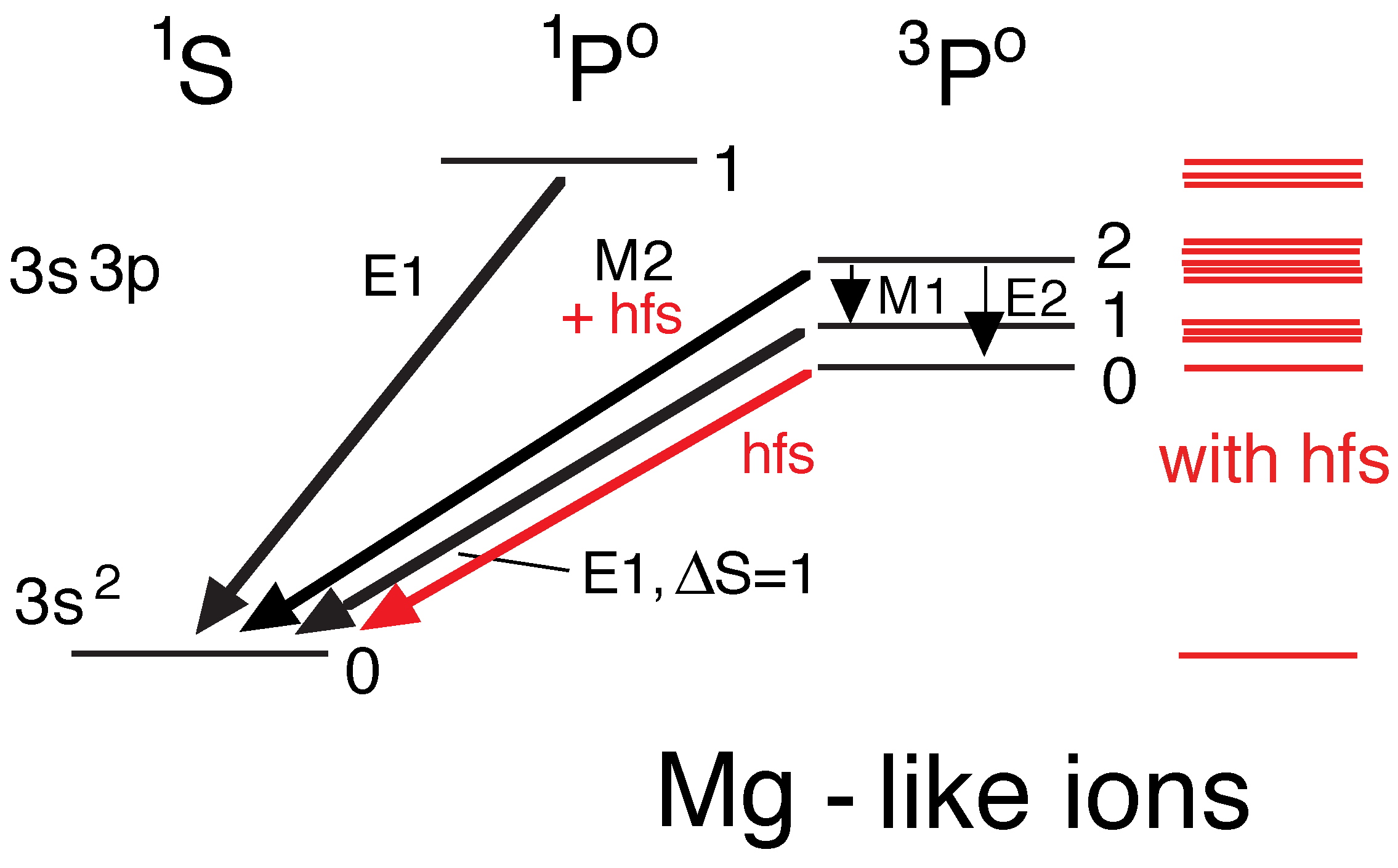
Figure 5.
Schematic (not to scale) of the lowest levels and transitions among levels of principal quantum number of C-like atomic systems. The numbers near the end of the level bars indicate the J value of the fine structure level. The lowest quintet level decays by spin-changing transition. All other transitions are -forbidden.

Figure 6.
Schematic (not to scale) of the lowest levels and -forbidden transitions among levels of the ground configuration of N-like ions. The J value of each level is indicated near the right-hand end of a level bar.
Figure 6.
Schematic (not to scale) of the lowest levels and -forbidden transitions among levels of the ground configuration of N-like ions. The J value of each level is indicated near the right-hand end of a level bar.

Figure 7.
Schematic (not to scale) of the lowest levels and -forbidden transitions among levels in the ground configuration of O-like ions. The J value of each level is indicated near the right-hand end of a level bar.
Figure 7.
Schematic (not to scale) of the lowest levels and -forbidden transitions among levels in the ground configuration of O-like ions. The J value of each level is indicated near the right-hand end of a level bar.

Figure 8.
Schematic (not to scale) of some of the -forbidden transitions among eight (out of 27 in total) levels in the lowest three configurations of Si-like ions. The J value of each level is indicated near the left-hand or right-hand end of a level bar. The figure indicates the three lowest electron configurations but shows only a few levels that belong to terms with long-lived levels. The magnetic quadrupole decays of the particularly long-lived level are marked in red.
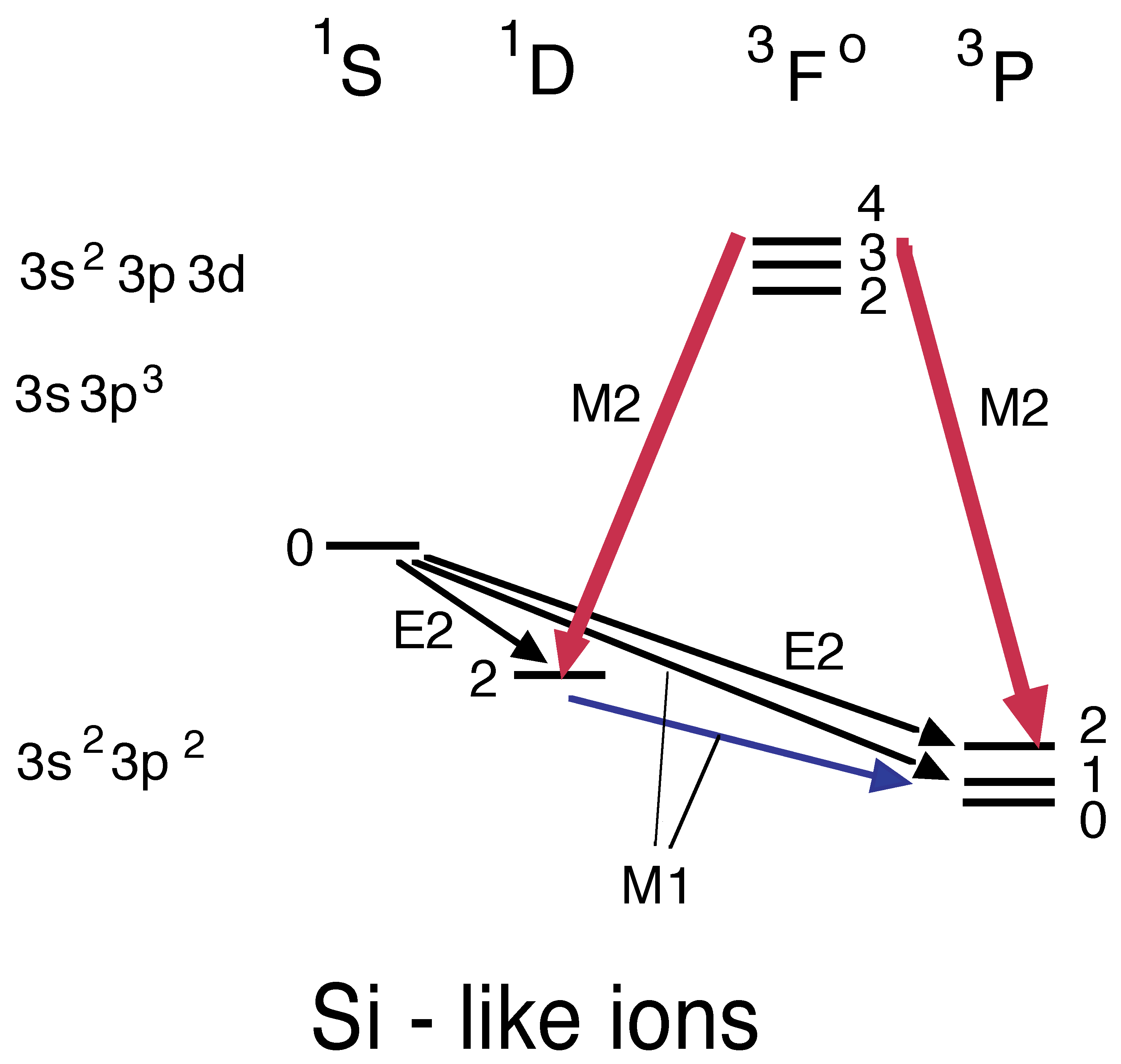
Figure 9.
Schematic of the lowest levels and -forbidden transitions among levels in Ar-like Fe (Fe IX) ions. Some transition multiplets have actually more components than are shown.
Figure 9.
Schematic of the lowest levels and -forbidden transitions among levels in Ar-like Fe (Fe IX) ions. Some transition multiplets have actually more components than are shown.
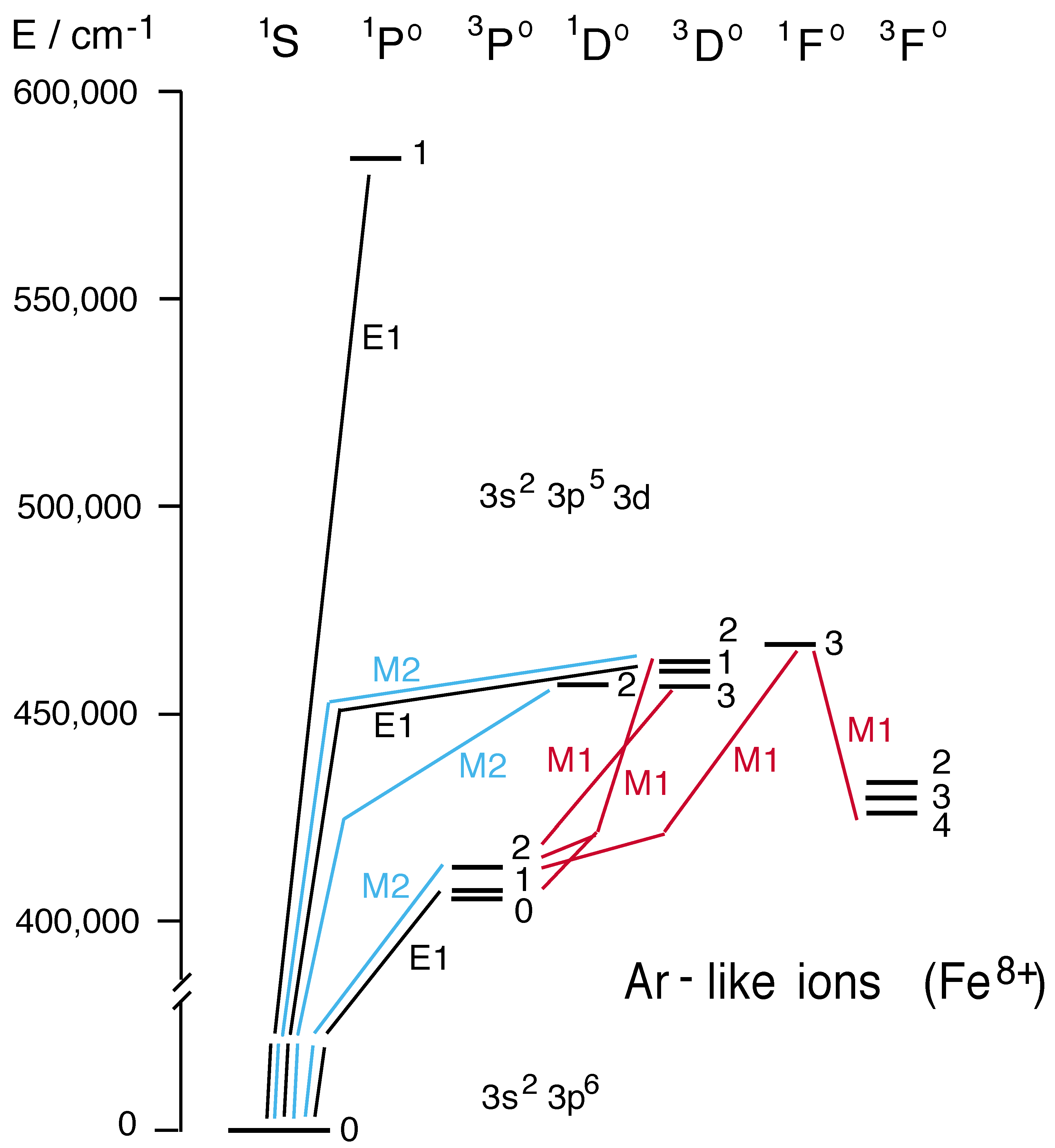
Disclaimer/Publisher’s Note: The statements, opinions and data contained in all publications are solely those of the individual author(s) and contributor(s) and not of MDPI and/or the editor(s). MDPI and/or the editor(s) disclaim responsibility for any injury to people or property resulting from any ideas, methods, instructions or products referred to in the content. |
© 2024 by the author. Licensee MDPI, Basel, Switzerland. This article is an open access article distributed under the terms and conditions of the Creative Commons Attribution (CC BY) license (https://creativecommons.org/licenses/by/4.0/).
Share and Cite
MDPI and ACS Style
Träbert, E. Long-Lived Levels in Multiply and Highly Charged Ions. Atoms 2024, 12, 12. https://doi.org/10.3390/atoms12030012
AMA Style
Träbert E. Long-Lived Levels in Multiply and Highly Charged Ions. Atoms. 2024; 12(3):12. https://doi.org/10.3390/atoms12030012
Chicago/Turabian StyleTräbert, Elmar. 2024. "Long-Lived Levels in Multiply and Highly Charged Ions" Atoms 12, no. 3: 12. https://doi.org/10.3390/atoms12030012
Note that from the first issue of 2016, this journal uses article numbers instead of page numbers. See further details here.