Abstract
Spectral line shapes code in plasmas (SLSPs) code comparison workshops have been organized in the last decade with the aim of comparing the spectra obtained with independently developed analytical and numerical models. Here, we consider the simultaneous effect of a plasma microfield and a periodic electric field on the hydrogen lines Lyman-α, Lyman-β, Balmer-α, and Balmer-β for plasma conditions where the Stark effect usually dominates line broadening.
1. Introduction
Recent advances in Stark profile modeling have resulted in a better agreement between theoretical and experimental spectra, and hence improved plasma parameter diagnostics. In the last few years, both analytical and numerical advances have made it possible to better explain some poorly understood features of line shapes. The spectral line shapes in plasmas workshops that began in 2012 [] allowed a comparison of the approaches used, included code cross-validation and improvement, and has helped to enrich the physical models used. Recent models retain high-order terms in the multipole expansion, going beyond a second-order approximation and including a quantum behavior of the perturbers [,]. Other developments concern the simultaneous effect of Stark and Zeeman broadening [,] and the effect of oscillating electric fields. Here, we report a comparison of several models for the effect of a periodic electric field , with a frequency and a random phase , assumed in the z direction. This is a basic oscillating electric field proposed in early approaches to model the effect of Langmuir waves on a line shape []. It has since been used in numerous works of the effect of plasma waves on atomic radiative properties [,]. For line shapes dominated by the Stark effect, an accurate calculation of the effect of periodic electric fields is of interest because in principle it allows for the simultaneous diagnostic of the plasma and oscillating field parameters. It is a difficult modeling problem since the time scales of the electronic, ionic, and oscillating fields are generally different.
At the sixth SLSP workshop, the simultaneous effect of the plasma microfield and an external harmonic field in a fixed direction have been investigated, assuming that the oscillating frequency is equal to the electronic plasma frequency , with , where is the electronic density, e and are the electron charge and mass, and is the permittivity of free space. Line shape calculations proposed for this workshop concern hydrogen Lyman-α, Lyman-β, Balmer-α, Balmer-β for the densities 1016 and 1017 cm−3, temperatures 1 and 10 eV, and the magnitude of the oscillating electric field equal to 0, 1, 3, and 10 , where:
is the Holtsmark field []. The densities and temperatures chosen for the code comparison are found in different kinds of laboratory plasmas such as stabilized arcs [] or toroidal devices []. One aim of the workshop is to improve the accuracy of the calculated line shapes for a given range of plasma conditions and identify how far one should go in the details of the modeling for reaching this accuracy. This workshop follows a similar comparison of codes calculating plasma opacity [], which showed the importance of using accurate line shapes for a reliable calculation of radiative transfer.
2. Models and Codes
The case definitions specify that the fine structure terms are neglected and that the dipole interactions are ignored, which means that only the dipolar elements between substates of the principal quantum number n contribute to the Stark effect of level n. Five codes (ERIP, HSTRKII, Mywave, SimU, Xenomorph) provided calculations for at least a part of the lines and the plasma conditions that were requested. We briefly describe the main features of these codes, which all use at least a computer simulation of ion dynamics. These simulations generate the time-dependent electric field felt by the atomic emitter, by summing at each time step the electric fields created by a large number of charged particles moving in a spherical, cylindrical, or cubic box—normally called the interaction or collision volume. The codes use different boundary conditions (if any), always with the aim of better reproducing the properties of real plasma. The simultaneous effect of the plasma microfield and the periodic electric field on the evolution of dipole radiation is obtained by numerically integrating the Schrödinger equation, a way of accurately capturing the complexity of atomic quantum dynamics.
In the code ERIP, the motion of the plasma electrons and ions is simulated with statistically independent charged particles moving on straight lines trajectories in a spherical box. Boundary conditions consist of a reinjection at a random point on the sphere and with a new velocity. The emitter is supposed to be fixed at the center of the sphere, with a μ-ion model used which attributes the perturber to the reduced mass of the emitter-perturber couple. The atomic state is described in terms of the Euler–Rodrigues parameters, allowing for an efficient calculation [].
The code HSTRKII is a flexible simulation code providing many options like the use of Euler–Rodrigues parameters or the addition of external fields. For periodic electric fields, specific analytical and numerical developments are available [] and were employed in the calculations. For the plasma simulation, the code uses the Hegerfeld–Kesting/Seidel method of collision-time statistics [] and computes the dipole autocorrelation C(t). The final line shape is obtained by a Fourier transform using Filon’s rule [].
The collision-time statistics method does not involve boundary conditions and reinjection, but instead considers all plasma particles that become relevant, i.e., come closer than three times the screening length, at any time in [0,T], with T representing the time when either the dipole autocorrelation function has become negligible, or an asymptotic (impact) tail is recognized. The method also computes the number of relevant particles to be simulated, with higher temperatures, and hence velocities, requiring more relevant particles.
It should be noted that HSTRKII does not assume stationarity. As a result, the expression for the autocorrelation function and the line shape is different. In the no-plasma limit, this results in the Blokhintsev expression [] for the line shape are:
where n and n’ are the principal quantum numbers for the upper and lower levels, respectively, and n1 and n2 are the parabolic quantum numbers for the upper level state, with the corresponding primed symbols for the lower state, the pth Bessel function of the first kind, δ as the Dirac δ-function and as the Bohr radius. In contrast, assuming stationarity, the corresponding expression is proportional to:
where is a radiative dipole element between an upper state α and lower state β, are the diagonal z-matrix elements in the parabolic basis for the states α and β, and Q = eF/ℏΩ. This difference shows up in a more pronounced, central satellite and correspondingly lower intensity p ≠ 0 satellites for HSTRKII.
Based on a simulation of independent quasiparticles with a Debye electric field, the code MyWave can potentially simulate both electrons and ions, but the profiles calculated for SLSP 6 use an electronic impact operator []. A few hundred particles move in a cubic box with straight path trajectories and basic periodic boundary conditions []. In addition to a periodic electric field, a fixed-direction magnetic field can be added for the diagnostic of magnetized plasmas []. The objective of the code is the simultaneous diagnostic of the plasma and oscillating electric fields properties in different kinds of plasmas.
SimU is a combination of two codes (though it can be run as a single executable, if desired): a molecular dynamics (MD) simulation of variable complexity, and a solver for the evolution of an atomic system with the MD field history used as a (time-dependent) perturbation. The main reference is [] with some more details in [].
Xenomorph is also a semi-classical calculation, where the electric field is obtained with a simulation of a large number of electrons and ions inside a sphere and a μ-ion model is used. If a particle leaves the simulation sphere, it is put back into the simulation with a new direction, velocity, and position. The new trajectory is selected from modified probability distributions which are weighted by the lifetime of the particle [].
For an overview of these five codes, we recall in Table 1 the main features of each code.

Table 1.
Summary of options used by the different codes.
3. Results
3.1. Overview of the Line Shapes Submitted
The SLSP workshop has developed a utility allowing the importing and submitting of cases, as well as analyzing the results submitted, and comparing them to the results of other codes []. For each of the four lines studied, sixteen line shapes, corresponding to the two densities and temperatures, and four values of the oscillating field magnitude have been submitted by at least three codes. The oscillating electric field is assumed to lie in the z direction, and the total line shape is calculated as the sum , where the π profiles correspond to radiative transitions with , and σ profiles to transitions with . We compare in the following total line shapes, but also in the and profiles. The profiles shown are mostly area normalized, and are plotted with frequencies in cm−1, around the frequency of the unperturbed line calculated neglecting fine structure. All of the calculated cases show line shapes that are very nearly symmetrical around the central frequency, as expected from the atomic physics model with a linear Stark effect and no fine structure. In the absence of an oscillating electric field, there is generally a very good agreement between the Lyman profiles. Differences depending on the plasma conditions appear for the line width of Balmer lines, and affect, in particular, calculations using the code MyWave. The impact approximation used in this code does not retain the upper and lower states interference term, thus overestimating the broadening. We discuss later for the Balmer-α case an additional difference linked with the use of an impact electronic operator and correlated with the appearance of non-impact effects in the action of electrons.
For all plasma conditions and lines calculated, profiles for an oscillating field magnitude F = F0 usually exhibit very small structures as near to the plasma frequency as can be seen by comparing to the corresponding F = 0 profile. For the cases F = 3F0 and F = 10F0, a first look reveals that the satellite structures located close to multiples of the plasma frequency appear on most of the profiles calculated. A closer look shows a difference in the size of these structures between the alpha lines (Lyman-α, Balmer-α), and the beta lines (Lyman-β, Balmer-β). It is then instructive to observe π and σ profiles separately: whereas beta lines exhibit significant structures on both π and σ profiles and alpha lines present such structures mainly for the π profiles, although low-intensity structures are visible on some σ Balmer-α profiles.
3.2. Lyman-α (Ly-α)
The Lyman-α line is well known to be affected by ion dynamics for a large range of laboratory plasma conditions, including the densities and temperatures calculated for the workshop. In view of the results shown in Figure 1 for a density Ne = 1017 cm−3, a temperature T = 10 eV, and an oscillating field with a magnitude F = 10F0, with four very similar line shapes obtained by four different codes, the simulation calculations seem to be able to give a reproducible and reliable picture of the simultaneous effect of the time-dependent plasma microfield and a periodic electric field.
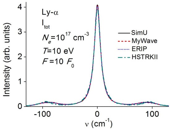
Figure 1.
Itot profiles of Ly-α calculated with the codes Simu, MyWave, ERIP, and HSTRKII in a periodic field of magnitude F = 10F0.
The difference between the and profiles appears clearly when comparing Figure 2 and Figure 3. Whereas two satellites are visible on on each side of the central component, at about one and two times the plasma frequency, no satellite appears on the profile. This is expected in terms of Equations (2) or (3), as the argument of Jp is 0 and only J0(0) = 1 is nonzero. The shape of Lyman-α is dominated by the presence of an undisplaced central component that is not affected by the oscillating electric field along z. This behavior may be understood by looking at the Lyman–α substates contributing to the central unshifted component. In a static picture, this central component originates from the substates m = ±1 of the state n = 2. In a static or dynamic picture, these states are not affected by an electric field along z.
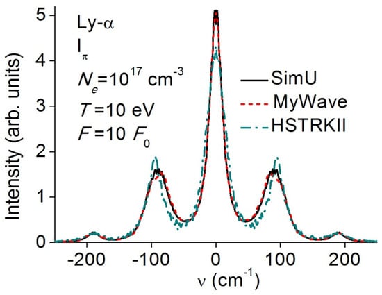
Figure 2.
Iπ profiles of Ly-α calculated with the codes Simu, MyWave, and HSTRKII in the conditions of Figure 1.
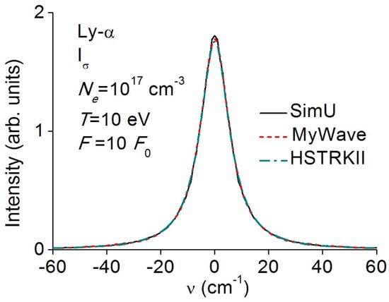
Figure 3.
Iσ profiles of Ly-α calculated with the codes Simu, MyWave, and HSTRKII in the conditions of Figure 1.
3.3. Balmer-α (Hα)
Although the energy level structure of Balmer-α is more complex than Lyman-α, a similar lack of interaction with the oscillating field is observed, resulting in a very small effect on the sigma components making up the central component. A comparison of the total line shapes plotted in Figure 4 for a density of Ne = 1016 cm−3 and a temperature of T = 10 eV shows a good overall agreement between the five codes. Remaining discrepancies of concern are, in particular, the broadening of the central component and the shape of the satellite structures. The code MyWave using an impact operator shows an additional broadening of about 15% as compared to the mean width value of the codes simulating electrons.
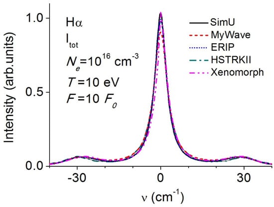
Figure 4.
Itot profiles of Hα calculated with the codes Simu, MyWave, ERIP, HSTRKII, and Xenomorph in a periodic field of magnitude F = 10F0.
The plasma conditions used in Figure 4, Figure 5 and Figure 6 justify the use of an impact collision operator for the electrons. Validity conditions for the use of this impact approximation imply that the electron collision time , with as the typical interparticle distance and as the electronic thermal velocity, remains small compared to the time of interest of the emitted radiation. A further condition for using a perturbative impact version is that the strong collisions, having impact parameters smaller than the electronic Weisskopf radius , remain rare events. A small ratio prevents the occurrence of such simultaneous strong collisions and validates the use of an impact operator. This ratio is equal to 0.02 for the conditions of Figure 4, Figure 5 and Figure 6 but reaches 0.13 for a line calculated with Ne = 1017 cm−3 and T = 1 eV, while it is of about 0.05 for the two other conditions used (Ne = 1016 cm−3 and T = 1 eV, Ne = 1017 cm−3 and T = 10 eV). For the lines plotted, the width of the line shape using an impact operator (code MyWave) is about 15% larger than the mean width obtained with codes simulating the electrons. This excess of broadening increases to almost a factor of 2 for a ratio , while it is of about 35% for an intermediate value of . This indicates the importance of retaining non-impact effects for obtaining an accurate line width and shows the benefits of using full ion and electron simulations.
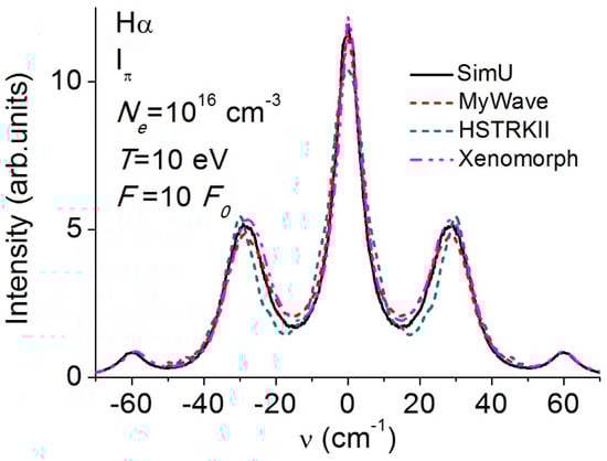
Figure 5.
Iπ profiles of Hα calculated with the codes SimU, MyWave, HSTRKII, and Xenomorph in a periodic field of magnitude F = 10F0.
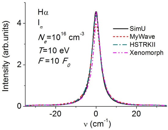
Figure 6.
Iσ profiles of Hα calculated with the codes SimU, MyWave, HSTRKII, and Xenomorph in a periodic field of magnitude F = 10F0.
3.4. Lyman-β (Ly-β)
The effect on Lyman-β of a periodic electric field in the same conditions as for Lyman-α in Figure 1, Figure 2 and Figure 3 clearly causes stronger changes on the line shape. The Itot line shapes plotted in Figure 7 demonstrate that there is a central satellite structure and at least three satellites around it on each side. The different codes are in good agreement, and all predict an intensity redistribution among the satellites. This effect is favored by the proximity between the plasma frequency and the average separation between Stark sub-levels, which induces a resonance effect between the emitter and the oscillating electric field.
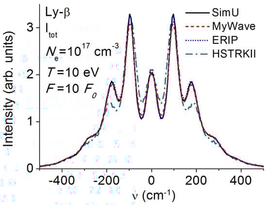
Figure 7.
Itot profiles of Ly-β calculated with the codes SimU, MyWave, ERIP, and HSTRKII in a periodic field of magnitude F = 10F0.
The lines in Figure 8 exhibit broad lines with a central satellite, but the most intense satellite is at 2 ωp. While there is almost no satellite at ωp, two other weak-intensity satellites can be seen as shoulders on the line wing at 3 and 4 ωp. For this line, the plotted in Figure 9 shows a narrower line, with satellites at the line center, a dominant satellite at ωp, and two weaker intensity satellites at 2 and 3 ωp.
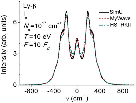
Figure 8.
Iπ profiles of Ly-β calculated with the codes SimU, MyWave, and HSTRKII in the conditions of Figure 7.
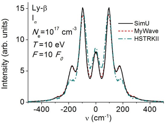
Figure 9.
Iσ profiles of Ly-β calculated with the codes SimU, MyWave, and HSTRKII in the conditions of Figure 7.
3.5. Balmerβ (Hβ)
The Balmer β profiles plotted in Figure 10 for a density Ne = 1016 cm−3 and a temperature T = 1 eV also show a good agreement between the five codes used, and as in the case of Lyman β, shows a significant redistribution of the Itot line among a central component and at least three satellites on each side for an oscillating field magnitude of . For the lines plotted in Figure 11, a small central component appears, as well as a weak intensity satellite at ωp, a large intensity satellite at 2 ωp, and two other weak intensity satellites at 3 and 4 ωp. In Figure 12, a central component is clearly visible on , with Lyman-β, the most intense satellite at ωp, and two other weaker satellites at 2 and 3 ωp.
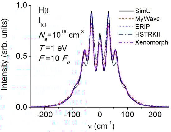
Figure 10.
Itot profiles of Hβ calculated with the codes SimU, MyWave, ERIP, HSTRKII, and Xenomorph in a periodic field of magnitude F = 10F0.
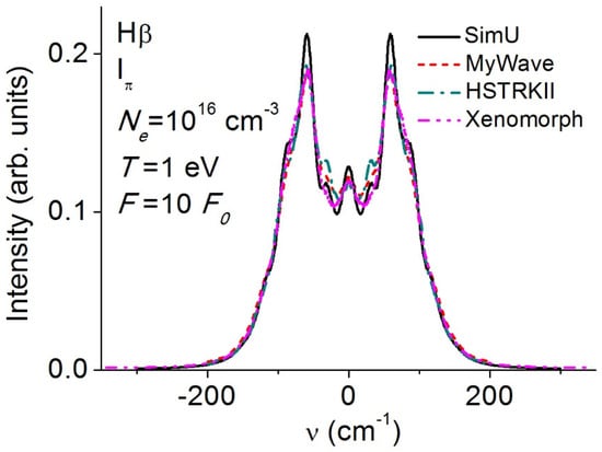
Figure 11.
Iπ profiles of Hβ calculated with the codes SimU, MyWave, HSTRKII, and Xenomorph in a periodic field of magnitude F = 10F0.
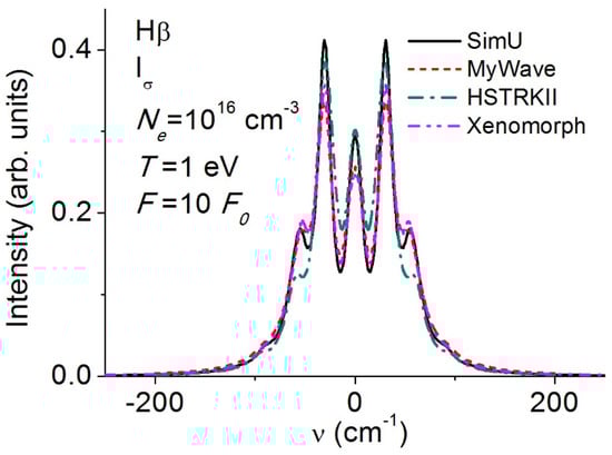
Figure 12.
Iσ profiles of Hβ calculated with the codes SimU, MyWave, HSTRKII, and Xenomorph in a periodic field of magnitude F = 10F0.
All of the line shapes presented so far have been calculated for a magnitude , which is larger than the mean plasma microfield. The satellites visible on these line shapes, which include the central components for the beta lines, result from the joint effect of the periodic field and the time-dependent microfield. In the absence of the plasma microfield, one would observe the early discovered Blokhintsev spectra [], where discrete satellites are separated by the oscillation frequency and have an intensity defined by Bessel functions Jp, with p the harmonic number defined by ω = p ωp. The intensity distribution of the satellites observed in Figure 7, Figure 8, Figure 9, Figure 10, Figure 11 and Figure 12 shares some of the characteristics of the Blokhintsev spectrum but is modified here by the time-dependent ion and electron microfield.
For the same plasma conditions as in Figure 10, Figure 11 and Figure 12, we show in Figure 13 the Itot Hβ for an oscillating field magnitude F = 3F0. Most of the calculations present a central dip which is often observed for this line in the absence of the periodic field. Here, the main effect of the periodic field is the appearance of a small-intensity satellite near the plasma frequency, as has been observed since the seventies in several experiments affected by Langmuir waves [,].
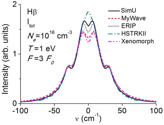
Figure 13.
Itot profiles of Hβ calculated with the codes SimU, MyWave, ERIP, HSTRKII, and Xenomorph in a periodic field of magnitude F = 3F0.
3.6. Line Shapes in Absence of Oscillating Electric Field
The hydrogen line shapes calculated in the absence of an oscillating electric field have been compared in detail during the five first SLSP workshops organized since 2012. The first workshop already showed that there was a reasonable agreement between the codes, with the exception of Lyman-α, for which a significant scatter of the width was observed []. It was then identified that the shape of Lyman-α is strongly influenced by ion dynamics, which affects the line by a change in the electric field magnitude and direction []. All of the five codes compared here use a computer simulation of the ion motion coupled with a numerical integration of the Schrödinger equation. This approach provides a realistic contribution of ion dynamics to the codes. In Figure 14, we plotted the Lyman-α line shape calculated without the oscillating electric field with four codes. The peak normalization allows us to better measure the small remaining width difference between the codes. Differences between the profiles calculated by the codes without oscillating electric fields can still be visible on Balmer lines. In Figure 15, we plotted the Hβ line for a density Ne = 1016 cm−3 and a temperature T = 1 eV. The remaining differences in the profiles concern the line widths, but also the central dip of this line for which all the components are shifted by the electric field. These differences can be attributed to the way in which one follows the dynamics of electron and ion electron fields, with e.g., the boundary conditions used. For the code MyWave, the use of a basic impact approximation clearly overestimates the broadening as discussed in Section 3.3. In summary, the small differences observed in the calculations of the lines in absence of an oscillating electric field do not seem to affect the strong changes observed in the line shapes calculated in the presence of a large periodic field.
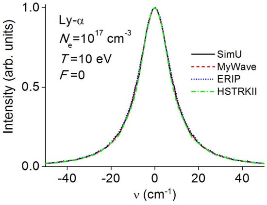
Figure 14.
Profiles of Ly-α calculated for F = 0 with the codes SimU, MyWave, ERIP, and HSTRKII for the density and temperature of Figure 1.
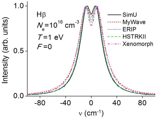
Figure 15.
Profiles of Hβ calculated for F = 0 with the codes SimU, MyWave, ERIP, HSTRKII, and Xenomorph for the density and temperature of Figure 10.
4. Conclusions
With the aim of analyzing the effect of a periodic electric field on hydrogen line shapes, we have compared the calculations of five different codes in four different plasma conditions. Satellite structures appear on the line shape close to multiples of the plasma frequency as soon as the magnitude of the oscillating electric field is of the order or larger than the Holtsmark microfield. The alpha line shapes are less affected than the beta lines for the conditions studied, and this can be understood by looking at the π and σ profiles of the lines studied. Codes using electron and ion simulations give remarkably consistent results and are also in good agreement with the code using an electronic impact operator, provided the conditions for the validity of this approximation are satisfied. Accurate calculations retaining the effect of periodic fields are of interest for different kinds of plasmas, and it would be interesting to compare such calculations to recent experimental data.
Author Contributions
Parentheses, formal analysis, software, validation, writing: I.H., S.A. and R.S. All authors have read and agreed to the published version of the manuscript.
Funding
This research received no external funding.
Data Availability Statement
The data that support the findings of this study are available from the corresponding author upon reasonable request.
Acknowledgments
The authors would like to thank the International Atomic Energy Agency for the scientific, technical and financial support of the SLSP workshop.
Conflicts of Interest
The authors declare no conflicts of interest.
References
- Stambulchik, E. Review of the 1st Spectral Line Shapes in Plasmas code comparison workshop. High Energy Density Phys. 2013, 9, 528–534. [Google Scholar] [CrossRef]
- Stambulchik, E.; Iglesias, C. Full radiator-perturber interaction in computer simulations of hydrogenic spectral line broadening by plasmas. Phys. Rev. E 2022, 105, 055210. [Google Scholar] [CrossRef]
- Gomez, T.; Nagayama, T.; Cho, P.; Zammit, M.; Fontes, C.; Kilcrease, D.; Bray, I.; Hubeny, I.; Dunlap, B.; Montgomery, M.; et al. All-order full-Coulomb quantum spectral line-shape calculations. Phys. Rev. Lett. 2021, 127, 235001. [Google Scholar] [CrossRef] [PubMed]
- Rosato, J.; Marandet, Y.; Stamm, R. A new table of Balmer line shapes for the diagnostic of magnetic fusion plasmas. J. Quant. Spectrosc. Radiat. Transf. 2017, 187, 333–337. [Google Scholar] [CrossRef]
- Ferri, S.; Peyrusse, O.; Calisti, A. Stark–Zeeman line-shape model for multielectron radiators in hot dense plasmas subjected to large magnetic fields. Matter Radiat. Extrem. 2022, 7, 015901. [Google Scholar] [CrossRef]
- Baranger, M.; Mozer, B. Light as a plasma probe. Phys. Rev. 1961, 123, 25–28. [Google Scholar] [CrossRef]
- Lisitsa, V. Atoms in Plasmas; Springer: Berlin/Heidelberg, Germany, 1994; ISBN 3-540-57580-4. [Google Scholar]
- Oks, E. Plasma Spectroscopy; Springer: Berlin/Heidelberg, Germany, 1995; ISBN 3-540-54100-4. [Google Scholar]
- Griem, H. Principles of Plasma Spectroscopy; Cambridge University Press: Cambridge, UK, 1997; ISBN 0-521-45504-9. [Google Scholar]
- Wiese, W.; Kelleher, D.; Paquette, D. Detailed study of the Stark broadening of Balmer lines in a high density plasma. Phys. Rev. A 1972, 6, 1132–1153. [Google Scholar] [CrossRef]
- Gallagher, C.; Levine, M. Observation of Hβ satellites in the presence of turbulent electric fields. Phys. Rev. Lett. 1971, 27, 1693–1696. [Google Scholar] [CrossRef]
- Rose, S. A review of opacity workshops. J. Quant. Spectrosc. Radiat. Transf. 1994, 51, 317–318. [Google Scholar] [CrossRef]
- Gigosos, M.; Fraile, J.; Torres, F. Hydrogen Stark profiles: A simulation-oriented mathematical simplification. Phys. Rev. A 1985, 31, 3509–3511. [Google Scholar] [CrossRef]
- Alexiou, S. Methods for Line Shapes in Plasmas in the Presence of External Electric Fields. Atoms 2021, 9, 30. [Google Scholar] [CrossRef]
- Hegerfeld, G.; Kesting, V. Collision time simulation technique for pressure-broadened spectral lines with applications to Ly-α. Phys. Rev. A 1988, 37, 1488–1496. [Google Scholar] [CrossRef]
- Tuck, E. A simple “Filon-trapezoidal” rule. Math. Comput. 1967, 21, 239–241. [Google Scholar]
- Blokhintsev, D. Theory of the Stark effect in a time-dependent field. Phys. Z. Sow. Union 1933, 4, 501–515. [Google Scholar]
- Griem, H.; Kolb, A.; Shen, K. Stark broadening of hydrogen lines in a plasma. Phys. Rev. 1959, 116, 4–16. [Google Scholar] [CrossRef]
- Hannachi, I.; Stamm, R.; Rosato, J.; Marandet, Y. Calculating the simultaneous effect of ion dynamics and oscillating electric fields on Stark profiles. Adv. Space Res. 2023, 71, 1269–1274. [Google Scholar] [CrossRef]
- Hannachi, I.; Stamm, R.; Rosato, J.; Marandet, Y. Spectroscopic diagnostic of oscillating electric fields in edge plasmas. Contrib. Plasma Phys. 2022, 62, e202100168. [Google Scholar] [CrossRef]
- Stambulchik, E.; Maron, Y. A study of ion-dynamics and correlation effects for spectral line broadening in plasma: K-shell lines. J. Quant. Spectrosc. Radiat. Transf. 2006, 99, 730–749. [Google Scholar] [CrossRef]
- Stambulchik, E.; Alexiou, S.; Griem, H.; Kepple, P. Stark broadening of high principal quantum number hydrogen Balmer lines in low-density laboratory plasmas. Phys. Rev. E 2007, 75, 016401. [Google Scholar] [CrossRef] [PubMed]
- Cho, P.; Gomez, T.; Montgomery, M.; Dunlap, B.; Fitz Axen, M.; Hobbs, B.; Hubeny, I.; Winget, D. Simulation of Stark-broadened hydrogen Balmer-line shapes for DA white dwarf synthetic spectra. ApJ 2022, 927, 70. [Google Scholar] [CrossRef]
- SLSP Browser Extension. Available online: https://plasma-gate.weizmann.ac.il/slsp/xul/ (accessed on 1 December 2022).
- Ramette, J.; Drawin, H. Structure of Stark Broadened Hβ Lines at low Electron Densities. Z. Naturforschung A 1976, 31, 401–407. [Google Scholar] [CrossRef]
- Rutgers, W.; de Kluiver, H. The dynamic Stark-effect in a turbulent hydrogen plasma. Z. Naturforschung A 1974, 29, 42–44. [Google Scholar] [CrossRef]
- Ferri, S.; Calisti, A.; Mossé, C.; Rosato, J.; Talin, B.; Alexiou, S.; Gigosos, M.; Gonzales, M.; Gonzales-Herrero, D.; Lara, N.; et al. Ion dynamics effect on Stark-broadened line shapes: A cross-comparison of various models. Atoms 2014, 2, 299–318. [Google Scholar] [CrossRef]
Disclaimer/Publisher’s Note: The statements, opinions and data contained in all publications are solely those of the individual author(s) and contributor(s) and not of MDPI and/or the editor(s). MDPI and/or the editor(s) disclaim responsibility for any injury to people or property resulting from any ideas, methods, instructions or products referred to in the content. |
© 2024 by the authors. Licensee MDPI, Basel, Switzerland. This article is an open access article distributed under the terms and conditions of the Creative Commons Attribution (CC BY) license (https://creativecommons.org/licenses/by/4.0/).