AtomPy: An Open Atomic Data Curation Environment for Astrophysical Applications

Abstract

We present a cloud-computing environment, referred to as AtomPy, based on Google-Drive Sheets and Pandas (Python Data Analysis Library) DataFrames to promote community-driven curation of atomic data for astrophysical applications, a stage beyond database development. The atomic model for each ionic species is contained in a multi-sheet workbook, tabulating representative sets of energy levels, A-values and electron impact effective collision strengths from different sources. The relevant issues that AtomPy intends to address are: (i) data quality by allowing open access to both data producers and users; (ii) comparisons of different datasets to facilitate accuracy assessments; (iii) downloading to local data structures (i.e., Pandas DataFrames) for further manipulation and analysis by prospective users; and (iv) data preservation by avoiding the discard of outdated sets. Data processing workflows are implemented by means of IPython Notebooks, and collaborative software developments are encouraged and managed within the GitHub social network. The facilities of AtomPy are illustrated with the critical assessment of the transition probabilities for ions in the hydrogen and helium isoelectronic sequences with atomic number $Z\le 10$.

1. Introduction

This report is concerned with problems of atomic data assessment and the development of cloud-computing tools to make it more efficient in the current data-intensive and collaborative research enterprise. In more than one way, two of us (C.M. and M.A.B) were early converts to this new scientific order, usually referred to as e-Science [1], by participating since the 1980s in the international Opacity Project (OP) [2,3] and Iron Project (IP) [4,5,6]. The OP was concerned with the computation of the massive atomic data required to estimate astrophysical opacities, while the IP computed large radiative and collisional datasets for plasma diagnostics based on iron-group ions. Data dissemination initiatives within these two consortia led to the development of some of the first online atomic databases, namely TOPbase [7,8,9] and TIPbase [10], and the astrophysical opacities web service referred to as OPserver [11,12].

Today e-Science is transforming the whole research cycle, especially data assessment methodologies due to the large volumes involved, distributed repositories with heterogeneous data models and the widespread use of innovative and sophisticated information and communication technologies (ICT) that are difficult to assimilate by traditional scientists [13,14,15]. Atomic data production is not alien to this revolution. We have seen, apart from the seminal nist (National Institute of Standards and Technology) Atomic Spectra Database [16,17], the proliferation of atomic databases: chianti [18,19,20], atomDB [21,22], uaDB [23], norad-Atomic-Data [24], the mchf/mcdhf database [25] and vald [26,27,28], to name a few. These databases vary greatly in terms of structure, data models and nomenclature. They also differ in data content, completeness, accuracy and provenance, and are hardly interoperable inasmuch as to facilitate user data searches. A remarkable attempt to improve integration and interoperability among atomic and molecular databases was launched in 2009 by the European Union: the Virtual Atomic and Molecular Data Centre (VAMDC) [29,30,31,32], aimed at implementing a cyberinfrastructure capable of interconnecting several (more than 15) of such databases. In this project an international group of physicists and computer scientists defined and implemented interoperability standards and protocols, virtual node architectures, XML schemata, query languages and web portals.

In spite of all these data activities, the issue of atomic data accuracy among astrophysical modelers remains inscrutable. The implementation of any spectral modeling code generally involves lengthy searches of atomic parameters in the aforementioned databases in order to piece together a master dataset as complete and accurate as possible. Such a task is usually reserved to experts capable of reviewing the available data, a job that may take up several years. There are many disadvantages to this approach: the master dataset becomes outdated even before its release; the process is expensive and unsustainable in the long term; newer atomic data are not taken into account and tested until they are incorporated into the databases; it is error-prone, from mistakes in data entry to expert misjudgment in data selection; there is scanty user feedback to the data producers and collectors; and a lot of the data are replaced, discarded or simply lost (together with the knowledge and investment that went into their production). With regards to expert judgment on the available atomic data, it must be emphasized that there are no exact solutions to multi-electron atomic structures; thus, atomic physicists must follow their own experience and rules of thumb when evaluating data worthiness from published papers, but that is no guarantee that the chosen datasets are indeed the most accurate.

To address some of these issues, we propose in Section 2 – Section 3 a new data curation model driven by an open virtual research community of both data producers and users. As a previous experience, the evaluation of oxygen atomic data presented in Appendix A of the book Oxygen in the Universe [33] was efficiently supported by open Google-Drive spreadsheets that avoided the clogging of the text with an excessive number of tables. We have therefore been encouraged to extend this approach to the implementation of a cloud-computing data curation environment, to be referred hereafter as AtomPy, based on the functionalities of both Google Sheets and Pandas (Python Data Analysis Library) DataFrames. This system is described in Section 4 and fully used to evaluate in Section 5 the radiative rates for ions in the hydrogen and helium isoelectronic sequences with atomic number $Z\le 10$. Finally, some conclusions and recommendations are discussed in Section 6.

2. Virtual Research Communities

Collaborative data-intensive science essentially lives in the virtual space (cyberspace) brought about by a second generation Internet, where the geographical distances between researchers and their everyday facilities (instrumentation, computers, libraries, editors, etc.) are no longer a limitation [34]. In addition to a marked increase in the number and scale of international research ventures, new patterns of collaboration are quickly emerging: social networks; virtual research communities (VRCs) and interdisciplinary research projects [35]. The new dynamics are characterized by alternative communication channels, different divisions of labor, standardization of working habits, collaborative continuity, competency matching, specialization and cooperation.

As shown in Figure 1, the VRC allows a dispersed but networked group of researchers to work together effectively through the use of ICT. Within VRC cyberspace, they share data, software tools, facilities and information resources, intercommunicating and producing joint results. The productivity of a VRC depends on the development of certain capabilities: community management; support for distributed research and collaboration; human–computer interfaces and interoperability that inevitably require an open and flexible middleware of computer tools and services [36].

The VRC, particularly one consisting of both data producers and users, offers singular potential for efficient and sustainable data assessment. It presents, in fact, a unique opportunity to nucleate and consolidate both camps using data quality as the new currency to debug and streamline the whole research chain. It must be mentioned that cohesiveness between atomic data producers and users has not been easy to broker in the past, in spite of periodic international conferences such as icamdata [37], joint symposia (e.g., the Tenerife meeting in October 2010 on “Uncertainties in atomic data and how they propagate in chemical abundances” [38,39]), capacity development schools (e.g., NebulAtom [40]), and the AstroAtom blog [41]. However, there are exceptions to this inherent detachment, in particular the extensive astrophysical benchmarks that have been carried out of iron EUV and X-ray lines for the chianti database [42,43,44,45,46,47,48,49,50,51,52,53,54,55,56].

Figure 1. Example of a virtual research community. Image source: Figure 1 of [36].

Figure 1. Example of a virtual research community. Image source: Figure 1 of [36].

3. Community-Driven Data Curation

With the onset of the data deluge, it was soon realized that the scale and complexity of scientific data would require active management during their complete life cycle in order to ensure trustworthiness, integrity, access, fitness for use and reusability [57,58,59]. These activities are now part of an emerging and growing discipline referred to as data curation dedicated to the present and future maximization of data potential, in particular of knowledge-centric data. It then becomes clear that the process of data assessment implies a stage beyond database development very much associated to the realms of this new field, which is the main concern of the present work.

In an extensive analysis of digital data curation [58], an integrated three-level model has been proposed to address the demands of e-Science (see Figure 2). The black arrows denote data pathways in the traditional research process (Level 1): primary data are used to derive secondary and tertiary data, the latter finally resulting in papers that are published in the usual peer review journals eventually reaching a wider audience (other scientists, general public, industry and libraries). Primary and secondary data may also be archived enabling alongside (red arrows) data-based research (Level 2) and, hopefully, new discoveries. A further level of long-term curation (Level 3) involves, apart from the Level-2 archives, more sophisticated and dynamic data repositories with extensive metadata and hyperlinks (blue arrows) to promote collection-based research. The traditional data archivist now becomes the data curator and the publication process experiments with alternative media. We are of the opinion that data assessment activities should be managed in Level 3 of this model.

Since data assessment is in general a long-term activity, it is limited by contemporary funding time scales that are mostly short-term and project-based; its sustainability is consequently always fragile. In this respect, we are exploring the feasibility of a self-sustainable model based on an open VRC as described in Section 2 and on community-driven data curation similar to Wikipedia [60], ChemSpider [61] and WikiGenes [62,63]. In a comprehensive analysis of this approach [64], its effectiveness is discussed when the availability of updated, large-scale and dynamic datasets is critical, and its success depends on several well-defined practices: data producer–user involvement; the promotion of outreach activities; member incentives and a governance model based on meritocracy. The need for robust and standardized data representations, a balance between human- and computer-based curation methods and for data provenance and preservation, is also therein emphasized. Moreover, the participation of the data users in the curation process is key to the development of modern repositories, and curation activities would need to start early in the research cycle [65]. This is certainly the case of atomic data where accuracy must be reinforced through diagnostic benchmarks carried out mostly by plasma modelers.

Figure 2. Three-level data curation model proposed for e-Science specifications. Image source: Figure 10 of [58].

Figure 2. Three-level data curation model proposed for e-Science specifications. Image source: Figure 10 of [58].

While Wikipedia uses the wiki as its main content building block, we propose the Google Sheet and its counterpart in the Python environment, the Pandas DataFrame, as the basic structures for data assessment due to their powerful and well-known data manipulation functions. Therefore, the AtomPy software is fairly simple: it is essentially confined to an Application Programming Interface (API) for data downloading from Google Drive to the user disk space and a series of Python utilities developed by community members to be shared in the GitHub [66] social network.

4. AtomPy

AtomPy is a cloud environment for atomic data curation rather than an atomic database in the sense that a prospective user, apart from being able to search for data, is encouraged to contribute with datasets and utilities to facilitate data interfaces, comparisons, assessments and, ultimately, preservation. The AtomPy [67] atomic data and metadata reside in spreadsheets in Google Drive (see Section 4.1), where they can be openly accessed, modified and downloaded by any user. Data downloading can be carried out through the different format options offered by Google Sheets (Section 4.2) or to local Pandas DataFrames (Section 4.3) by means of the AtomPy API (Section 4.4) for further manipulation. Data uploading by prospective contributors to existing or new spreadsheets is at present managed through the usual Google-Drive channels. In order to facilitate user interaction, workflows for different data manipulation procedures are to be implemented with IPython notebooks (Section 4.5), which can be accessed from the GitHub repository (Section 4.6); that is, the end user is especially encouraged to contribute to the notebook and module pools in GitHub. Details of the installation of the AtomPy Python modules are given in Section 4.7.

4.1. AtomPy Spreadsheet Structure

AtomPy contains three reference spreadsheets with useful atomic information:

elements—lists the names, symbols and atomic weights for chemical elements indexed with the atomic number $Z\le 118$;

ions—lists the symbol, ground electronic configuration, ground spectroscopic term, total angular momentum (J) and ionization potential (in eV) for each ionic species indexed with the atomic number and electron number tuple $(Z,N)$, where $1\le Z\le 110$ and $1\le N\le Z$;

isotopes—lists symbols, atomic weights and fractions for isotopes indexed with the atomic number and mass number tuple $(Z,M)$ for $Z\le 118$.

In Figure 3 we show the ions sheet where it may be appreciated that, for each ionization potential, its value and uncertainty are both given. The source reference, in this case nist, is also specified and hyperlinked.

The atomic data (energy levels, radiative A-values, collision strengths and electron effective collision strengths) for ionic species $(Z,N)$ are stored in the Google workbook zz_nn.Xi, where zz and nn are two-character strings respectively associated to the atomic and electron numbers. X denotes the spreadsheets included in this workbook:

• E—contains the level energies of the atomic model;
• A—contains the radiative transition probabilities (A-values) and, in some cases, f-values;
• O—lists energy tabulations of collision strengths;
• U—lists temperature tabulations of effective collision strengths.

There may be more than one spreadsheet for each data type (i.e., i=0,1... where i=0 is the default); for example, when $LS$ and intermediate-coupling atomic models are both considered or when allowed and forbidden transitions are analyzed separately. Each ionic workbook is displayed in both the IsonuclearSequences/zz and IsoelectronicSequences/nn subdirectories of AtomPy. An important point here is the selected atomic model for each species that is mainly determined by astrophysical requirements, and is limited to a set of levels for which both radiative and collisional data have been reported.

The workbook for He i, for example, is labeled 02_02. In Figure 4 we show: (i) the 02_02.E0 spreadsheet listing level energies for a 49-level atomic model and (ii) 02_02.A0 with A-values for transitions with upper level $k\le 7$. The key advantage of AtomPy in data evaluation with respect to regular atomic databases is that for each atomic attribute—e.g., level energies $E(Z,N,i)$ or radiative transition probabilities $A(Z,N,k,i)$ (see indexing in E0 and A0)—it displays side by side values from several sources, which can then be statistically or graphically compared using the versatile functions of spreadsheets and DataFrames. Furthermore, the general policy is not to replace older datasets as new ones appear, thus contributing to data preservation for future reuse.

Figure 3. Google reference sheet ions of AtomPy listing NIST ionization potentials (IP) for elements with $Z\le 110$ (only those with $Z\le 8$ are displayed). Note that IP uncertainties are also included.

Figure 3. Google reference sheet ions of AtomPy listing NIST ionization potentials (IP) for elements with $Z\le 110$ (only those with $Z\le 8$ are displayed). Note that IP uncertainties are also included.

Figure 4. Workbook 02_02 for the $(2,2)$ ionic system (i.e., He i) showing the 02_02.E0 sheet with a 49-level atomic model (only the first 15 levels are depicted) and the 02_02.A0 sheet with A-values for transitions with upper level $k\le 7$.

Figure 4. Workbook 02_02 for the $(2,2)$ ionic system (i.e., He i) showing the 02_02.E0 sheet with a 49-level atomic model (only the first 15 levels are depicted) and the 02_02.A0 sheet with A-values for transitions with upper level $k\le 7$.

4.2. Google Sheets

The data processing capabilities of AtomPy are boosted by the paramount functionality of Google Sheet [68], essentially a cloud web-based spreadsheet application and data repository. Its functions regarding data manipulation, formatting and exporting, formula editing and chart plotting are comparable to the more familiar desktop spreadsheet packages; but additionally, it opens up new attractive possibilities for the VRC dynamics and community-based data curation described in Section 2 and Section 3:

• Simultaneous distributed editing;
• URL access;
• Dynamic embedding in websites and blogs.

Google Sheets offer different data sharing profiles, but to comply with the precepts of Section 3, full open access with editing capabilities has been adopted. Therefore, one could easily envision a geographically distributed group of researchers jointly evaluating, in real time, data tabulated in a single, common, editable spreadsheet stored in the cloud and displayed at each member’s site through a web browser. URL access has also enabled, through the HyperText Transfer Protocol (HTTP), the development of the AtomPy API, which is described in Section 4.4. On the other hand, Google Sheets do have data volume restrictions and the user may complain about poor response times, but in our opinion, its other positive features amply compensate for its present shortcomings.

4.3. Pandas DataFrames

The Python Data Analysis Library (Pandas [69]) provides high-level data structures and computer tools for large-scale data analysis and modeling in the Python environment, and is built on top of the NumPy package for high-performance scientific computing. Within Pandas, DataFrames are two-dimensional spreadsheet-like data structures with integrated indexing. In a similar fashion to spreadsheets, they provide extensive built-in functions for data manipulation; e.g., selection, filtering, indexing and re-indexing, mapping, sorting, ranking, uploading, storage, plotting and entry dropping. In practice, DataFrames would facilitate interfacing with modeling codes, particularly if model sensitivity to different atomic datasets is to be regularly tested.

4.4. API

The AtomPy API allows the user to download data from the Google-Drive cloud space into local Python data structures, in particular tuples and DataFrames. Its modules reside in both the Python Package Index (PyPI [70]) and GitHub [71] repositories from where they can be downloaded for local use (see Section 4.7 for details regarding installation and module dependencies).

AtomPy is invoked within a Python shell or IPython [72] interactive environment (see Section 4.5) with the command

In [1]: import atompy
Initializing AtomPy...
AtomPy ready!

Data from the elements, ions and isotopes reference sheets (see Section 4.1) can be addressed with commands of the type

In [2]: atompy.element(2)
Out[2]: ('Helium', 'He')

to list the name and symbol of the chemical element with atomic number $Z=2$ , or its atomic weight

In [3]: atompy.elementaw(2)
Out[3]: (4.002602, 2e-06)

It must be noted that the system returns a tuple rather than a single datum that includes, in the case of the atomic weight, both its nominal value and uncertainty. For the He i system, $(Z,N)=(2,2)$, ions would provide

In [4]: atompy.ion(2,2)
Out[4]: (′He I′, ′1s2′, ′1Se′, 0.0)
In [5]: atompy.ionip(2,2)
Out[5]: (24.587387936, 2.5e-08)

the latter tuple giving its ionization potential.

The He i workbook 02_02, for instance, can be downloaded to a local DataFrame (df) with the command

In [6]: df=atompy.getdata(2,2)
Retrieving workbook: 02_02
Finished workbook: 02_02
Ion: Z = 02, N = 02
  E0: Fine-Structure Energy Levels for He I
  E1: LS Energy Terms for He I
  A0: A-values for fine-structure transitions in He I
  A1: A-values for LS Transitions in He II
  U0: Effective Collision Strengths for LS Transitions of He I
  No O sheets found...

The local df DataFrame now contains data for four spreadsheets, namely E0, A0, A1 and U0. Attributes for the first 10 levels of E0, for example, can be listed with the Pandas command

In [7]: df.E(0)[:10]
Out[7]:
         Conf  Term  2S+1 L Pi J           E_S1     E_S2
Z N i
2 2 1    1s2   1S       1 0  0 0       0.000000      0.0
    2  1s.2s   3S       3 0  0 1  159855.974330 159831.0
    3  1s.2s   1S       1 0  0 0  166277.440141 166259.0
    4  1s.2p  3P*       3 1  1 2  169086.766472 169064.9
    5  1s.2p  3P*       3 1  1 1  169086.842898 169065.0
    6  1s.2p  3P*       3 1  1 0  169087.830813 169066.0
    7  1s.2p  1P*       1 1  1 1  171134.896946 171113.8
    8  1s.3s   3S       3 0  0 1  183236.791700 183216.9
    9  1s.3s   1S       1 0  0 0  184864.829320 184848.0
    10 1s.3p  3P*       3 1  1 2  185564.561920 185546.5

Each level in the E0 DataFrame is indexed with the tuple $(Z,N,i)$ , which allows further data selection; for instance, the energies of the first five levels from source S1 (spectroscopic values) are listed with the command

In [8]: df.E(0).ix[(2,2,1):(2,2,5)][′E_S1′]
Out[8]:
Z  N  i
2  2  1         0.000000
      2    159855.974330
      3    166277.440141
      4    169086.766472
      5    169086.842898
Name: E_S1, dtype: float64

The A-values for the electric dipole (E1) transitions in sheet A0 for source “S5” are obtained with

In [9]: df.A(0).ix[(2,2,1):(2,2,7)][′AE1_S5′]
Out[9]:
Z  N  k  i
2  2  2  1             NaN
      3  1             NaN
      4  1             NaN
         2    1.021300e+07
      5  1    1.775780e+02
         2    1.021300e+07
         3    2.689700e-02
      6  2    1.021300e+07
      7  1    1.798320e+09
         2    1.548935e+00
         3    1.974850e+06
Name: AE1_S5, dtype: float64

where each transition is now indexed with the tuple $(Z,N,k,i)$ . It may be seen that the DataFrame structure can handle empty items labeling them with NaN. Furthermore, the metadata for the source references in A0 can also be obtained with a similar command

In [10]: df.A(0,sources=True)
S4: comprehensive tabulation by Wiese, W.L.; Fuhr, J.R.
http://adsabs.harvard.edu/abs/2009JPCRD..38..565W
S2: Atomic structure calculations using MCHF and BSR. Zatsarinny, O.;
Froese Fischer, C.
http://adsabs.harvard.edu/abs/2009CoPhC.180.2041Z
S5: Relativistic calculations by Morton, D.C.; Drake, G.W.F.
http://adsabs.harvard.edu/abs/2011PhRvA..83d2503M
and Morton, D.C.; Moffatt, P.; Drake, G.W.F.
http://adsabs.harvard.edu/abs/2011CaJPh..89..129M
S8: Calculation with correlated variational wave functions of the Hylleraas
type. Drake, G.W.F.
http://adsabs.harvard.edu/abs/1986PhRvA..34.2871D
Level indices relative to E0

We have tried to give in this section a brief overall view of the possibilities of AtomPy in the Python sphere. What must be emphasized is that most of the data manipulation commands that have been shown—and there are many more—actually belong to Pandas rather than to our API; hence, the latter is a fairly concise yet powerful piece of software with the intention of promoting further module development by both atomic data producers and users.

4.5. IPython Notebook

Due to large and diverse data volumes and the mushrooming of distributed repositories, the introduction of scalable methods for data management and analysis such as workflow tools are becoming a pivotal feature [73,74]. A workflow is the blueprint of a multi-step scientific process that facilitates its automation, validation and reproduction, and therefore must integrate a cadre of distributed computational services, applications and databases without the need of relocation and low-level programming.

There are several workflow tools currently available, but in the present context we have implemented and recommend the IPython Notebook [75] (installation details are given in Section 4.7). It is a web-based interactive computational environment for writing documents that includes hypertext, mathematics, graphs, images, video and, most importantly, dynamic input/output data and code execution. Such documents can then be shared, run and modified by a community of users that are more interested in pursuing scientific endeavors than getting immersed in the technical aspects of the procedures involved. A Notebook file (myfile.ipynb, say) can be imported and run locally in the IPython shell with the command

ipython notebook myfile

or displayed as a static web page with the IPython Notebook Viewer [76].

Interactive instructions for running AtomPy, or any other utility that makes use of its API, written in the Notebook format can be stored in the AtomPy GitHub repository (see Section 4.6) for general downloading.

4.6. GitHub

A salient feature of data-intensive science is that the end user has evolved from the isolated individual to become a social network, and GitHub [66] is essentially a social network of programmers that offers software repositories (both public and private), code sharing, publishing services and project management tools for collaborative code development. It is built around the Git version control system, and its functionality is based on three methods: the fork, the pull request and the merge. Forking allows the copying of a repository from one account to another such that its code can be modified at will. If the intention is to share the new changes, a pull request is made to the primal owner who can then decide to merge them into the mainstream project.

As previously discussed (see Section 2 and Section 3), the idea behind AtomPy is to promote joint activities among the atomic data-producer and astrophysical communities where the sharing of data processing utilities is among the most attractive. In this respect, the AtomPy API can then be a pipeline between the atomic data worksheet repositories and prospective spectral modeling codes.

4.7. API Installation

Activation of the AtomPy API requires beforehand installation of the familiar scientific Python modules NumPy [77], SciPy [78] and Pandas [79]. It can then be easily downloaded from the Python Package Index (PyPI) and installed locally with the pip [80] command

pip install atompy

that resolves further module dependencies; alternatively, it can also be accessed from the GitHub repository with

pip install git+https://github.com/AtomPy/AtomPy

AtomPy updating requires uninstalling the current version on the user local disk before proceeding with the above commands, that is

pip uninstall atompy

In a similar fashion, IPython can be installed with the command

pip install ipython

which should take care of all the prerequisites for the Notebook option.

5. Radiative Data Assessment

We are interested in compiling and assessing atomic models containing both radiative and collisional data for astrophysical applications. Therefore, the number of energy levels in the models is determined on the one hand by user requirements and, on the other, by what is actually available from the data producers who have attended such a demand; for the simpler systems, this is usually limited to electron configurations with principal quantum number $n\le 5$. To illustrate the possibilities of AtomPy, we review here the fairly large datasets of level energies and radiative rates that have been computed for ions of the hydrogen and helium isoelectronic sequences with $Z\le 10$ by means of well-established structure and scattering codes: the Breit–Pauli, configuration-interaction (CI) superstructure [81], autostructure [82,83] and civ3 [84]; the multiconfiguration Hartree–Fock mchf [85]; the multiconfiguration Dirac–Fock grasp [86]; and the electron–ion scattering R-matrix package in both its $LS$ and intermediate coupling (IC) versions [87].

5.1. H Sequence

Highly accurate radiative transition probabilities for both allowed and forbidden lines of the hydrogen isotopes (H, D and T) have been critically compiled by Wiese and Fuhr [88], who recommend scaling laws for other members of the H isoelectronic sequence with low Z. Also, a noteworthy measurement in one-electron systems is the lifetime of the ${2\mathrm{p}}_{1/2}$ level in He ii at $99.717\pm 0.075$ ps, which is in excellent agreement with theory (99.6891 ps) thus confirming basic radiation theory at the 0.075% level [89].

Our intention here is to evaluate the accuracy of reported A-values for H-like systems with $(Z,N)=(1,1)$, $(2,1)$ and $(6-11,1)$ computed in IC with superstructure in the context of photoionization–recombination calculations [90,91,92,93,94,95,96] (these datasets are available online from the norad-Atomic-Data database [24], norad hereafter) and with grasp as target quality indicators for electron–ion scattering for $(7-11,1)$ [97] and $(1-10,1)$ [98]. These two grasp calculations yield very similar A-values, although the former did not consider E3 and M3 transitions and gives level energies with and without quantum electrodynamic (QED) corrections. These datasets are located in the $zz\_01$ workbooks ($zz=01,02,...,10$) listed in the AtomPy IsoelectronicSequences/01 subdirectory.

Since the relativistic A-values for E1 transitions listed in the online tables [99] of Jitrik and Bunge [100,101] agree with those in [88] to five significant figures and provide a more complete treatment of the forbidden transitions, we adopt their datasets as the standard for comparison. The relativistic A-values in [102] are not included in this study since only E1 transitions for selected ions were therein considered, neither will the two independent relativistic calculations [103,104] on the $2\mathrm{s}-1\mathrm{s}$ two-photon transition as they are in almost perfect accord.

Table 1. Average permyriad ($1/{10}^4$) differences between the A-values computed with grasp [98] for hydrogenic ions and the standard [100,101]. Allowed (E1) and forbidden (E2, E3, M1, M2 and M3) transitions between levels with principal quantum number $n\le 5$ in $(Z,N)=(1-7,1)$ are considered.

Ion	$A(Z,N)$	E1	E2	E3	M1	M2	M3
H i	$A(1,1)$	6	6	6	500	6	6
He ii	$A(2,1)$	4	2	2	90	2	2
Li iii	$A(3,1)$	5	1	2	85	2	2
Be iv	$A(4,1)$	3	1	2	62	1	1
B v	$A(5,1)$	2	1	2	13	1	1
C vi	$A(6,1)$	2	1	1	12	1	1
N vii	$A(7,1)$	1	1	1	3	1	1

Table 1. Average permyriad ($1/{10}^4$) differences between the A-values computed with grasp [98] for hydrogenic ions and the standard [100,101]. Allowed (E1) and forbidden (E2, E3, M1, M2 and M3) transitions between levels with principal quantum number $n\le 5$ in $(Z,N)=(1-7,1)$ are considered.

Ion	$A(Z,N)$	E1	E2	E3	M1	M2	M3
H i	$A(1,1)$	6	6	6	500	6	6
He ii	$A(2,1)$	4	2	2	90	2	2
Li iii	$A(3,1)$	5	1	2	85	2	2
Be iv	$A(4,1)$	3	1	2	62	1	1
B v	$A(5,1)$	2	1	2	13	1	1
C vi	$A(6,1)$	2	1	1	12	1	1
N vii	$A(7,1)$	1	1	1	3	1	1

In Table 1, we tabulate average relative differences between the A-values computed with grasp [98] for transitions involving levels with principal quantum number $n\le 5$ in H-like ions ($Z\le 7$) and those in the standard datasets [100,101]. In this comparison, we only include transitions with $logA(Z,N,k,i)>-10$, and excellent agreement (a few parts in ${10}^4$) is found except for M1 transitions. For H-like ions with low Z, such transitions have very small line strengths and, thus, very small A-values; furthermore, the M1 transition operator in some of the computer packages is coded in its exact relativistic form, while in others the Breit two-body corrections are added to the zero-order term

$${\mathbf{Q}}^{\mathbf{0}}=\sum _m^N\mathbf{l}\left(m\right)+{\sigma }_m$$

(1)

where $\mathbf{l}\left(m\right)$ is the $m^{\mathrm{th}}$ electron angular momentum operator and ${\sigma }_m$ is twice its spin operator [105,106]. These higher order corrections can lead to remarkable contributions (orders of magnitude in some cases) to the matrix element in H-like systems. In particular, four M1 transitions, namely ${4\mathrm{s}}_{1/2}-{3\mathrm{d}}_{3/2}$, ${5\mathrm{s}}_{1/2}-{3\mathrm{d}}_{3/2}$, ${5\mathrm{s}}_{1/2}-{4\mathrm{d}}_{3/2}$ and ${5\mathrm{p}}_{3/2}-{4\mathrm{f}}_{5/2}$, have very small A-values ($logA{(1,1,k,i)}_{\mathrm{M}1}<-14$) showing discrepancies as large as an order of magnitude. It may also be appreciated in Table 1 that the differences subside as Z increases, and by $Z>7$ they are expected to be less than 1 part in ${10}^4$.

Table 2. Problematic A-values (s${}^{-1}$) for E3, M2 and M1 forbidden transitions in H i. jb: standard reference [100,101]. grasp: computed with grasp [98]. norad: computed with superstructure [96] and listed in the norad database. autos: computed with autostructure in the present work. Note: $a\mathrm{E}\pm n\equiv a\times {10}^{\pm b}$.

$A(Z,N,k,i)$	jb	grasp	norad	autos
$A{(1,1,{3\mathrm{d}}_{5/2},{2\mathrm{p}}_{1/2})}_{\mathrm{E}3}$	1.2575E−05	1.2582E−05	1.96E−05	1.258E−05
$A{(1,1,{3\mathrm{d}}_{5/2},{2\mathrm{p}}_{1/2})}_{\mathrm{M}2}$	3.9297E−05	3.9319E−05	1.57E−04	3.932E−05
$A{(1,1,{4\mathrm{p}}_{1/2},{3\mathrm{d}}_{5/2})}_{\mathrm{M}2}$	4.6585E−08	4.6610E−08	1.87E−07	4.661E−08
$A{(1,1,{4\mathrm{d}}_{5/2},{2\mathrm{p}}_{1/2})}_{\mathrm{M}2}$	2.2848E−05	2.2861E−05	9.14E−05	2.286E−05
$A{(1,1,{4\mathrm{d}}_{5/2},{3\mathrm{p}}_{1/2})}_{\mathrm{M}2}$	5.2400E−07	5.2429E−07	2.10E−06	5.243E−07
$A{(1,1,{4\mathrm{f}}_{7/2},{3\mathrm{d}}_{3/2})}_{\mathrm{M}2}$	1.2319E−06	1.2326E−06	4.93E−06	1.233E−06
$A{(1,1,{3\mathrm{p}}_{1/2},{2\mathrm{p}}_{3/2})}_{\mathrm{M}1}$	1.2886E−08	1.2897E−08	1.42E−08	1.416E−08
$A{(1,1,{3\mathrm{d}}_{3/2},{1\mathrm{s}}_{1/2})}_{\mathrm{M}1}$	6.9292E−09	6.7907E−09	1.93E−08	1.036E−08
$A{(1,1,{3\mathrm{d}}_{3/2},{2\mathrm{s}}_{1/2})}_{\mathrm{M}1}$	1.0479E−10	1.0501E−10	2.02E−10	1.339E−10
$A{(1,1,{3\mathrm{p}}_{3/2},{2\mathrm{p}}_{1/2})}_{\mathrm{M}1}$	3.3801E−09	3.3816E−09	2.95E−09	2.949E−09
$A{(1,1,{4\mathrm{p}}_{1/2},{2\mathrm{p}}_{3/2})}_{\mathrm{M}1}$	7.5163E−09	7.5361E−09	8.45E−09	8.452E−09
$A{(1,1,{4\mathrm{p}}_{1/2},{3\mathrm{p}}_{3/2})}_{\mathrm{M}1}$	5.3686E−10	5.3726E−10	5.58E−10	5.580E−10
$A{(1,1,{4\mathrm{s}}_{1/2},{1\mathrm{s}}_{1/2})}_{\mathrm{M}1}$	5.3029E−07	5.1953E−07	5.32E−07	5.305E−07
$A{(1,1,{4\mathrm{d}}_{3/2},{1\mathrm{s}}_{1/2})}_{\mathrm{M}1}$	4.3213E−09	4.8205E−09	1.23E−08	6.533E−09
$A{(1,1,{4\mathrm{d}}_{3/2},{2\mathrm{s}}_{1/2})}_{\mathrm{M}1}$	6.0462E−11	6.1245E−11	1.31E−10	8.091E−11
$A{(1,1,{4\mathrm{d}}_{3/2},{3\mathrm{s}}_{1/2})}_{\mathrm{M}1}$	5.3957E−13	5.4042E−13	8.59E−13	6.385E−13
$A{(1,1,{4\mathrm{d}}_{3/2},{3\mathrm{d}}_{5/2})}_{\mathrm{M}1}$	5.4500E−11	5.4461E−11	5.95E−11	5.948E−11
$A{(1,1,{4\mathrm{p}}_{3/2},{2\mathrm{p}}_{1/2})}_{\mathrm{M}1}$	1.7386E−09	1.7351E−09	1.45E−09	1.446E−09
$A{(1,1,{4\mathrm{p}}_{3/2},{3\mathrm{p}}_{1/2})}_{\mathrm{M}1}$	1.9206E−10	1.9206E−10	1.83E−10	1.833E−10
$A{(1,1,{4\mathrm{d}}_{5/2},{3\mathrm{d}}_{3/2})}_{\mathrm{M}1}$	1.4421E−11	1.4318E−11	1.23E−11	1.232E−11
$A{(1,1,{4\mathrm{f}}_{5/2},{2\mathrm{p}}_{3/2})}_{\mathrm{M}1}$	4.3994E−11	4.3919E−11	9.17E−11	5.231E−11
$A{(1,1,{4\mathrm{f}}_{5/2},{3\mathrm{p}}_{3/2})}_{\mathrm{M}1}$	1.4489E−12	1.4493E−12	2.40E−12	1.620E−12

Table 2. Problematic A-values (s${}^{-1}$) for E3, M2 and M1 forbidden transitions in H i. jb: standard reference [100,101]. grasp: computed with grasp [98]. norad: computed with superstructure [96] and listed in the norad database. autos: computed with autostructure in the present work. Note: $a\mathrm{E}\pm n\equiv a\times {10}^{\pm b}$.

$A(Z,N,k,i)$	jb	grasp	norad	autos
$A{(1,1,{3\mathrm{d}}_{5/2},{2\mathrm{p}}_{1/2})}_{\mathrm{E}3}$	1.2575E−05	1.2582E−05	1.96E−05	1.258E−05
$A{(1,1,{3\mathrm{d}}_{5/2},{2\mathrm{p}}_{1/2})}_{\mathrm{M}2}$	3.9297E−05	3.9319E−05	1.57E−04	3.932E−05
$A{(1,1,{4\mathrm{p}}_{1/2},{3\mathrm{d}}_{5/2})}_{\mathrm{M}2}$	4.6585E−08	4.6610E−08	1.87E−07	4.661E−08
$A{(1,1,{4\mathrm{d}}_{5/2},{2\mathrm{p}}_{1/2})}_{\mathrm{M}2}$	2.2848E−05	2.2861E−05	9.14E−05	2.286E−05
$A{(1,1,{4\mathrm{d}}_{5/2},{3\mathrm{p}}_{1/2})}_{\mathrm{M}2}$	5.2400E−07	5.2429E−07	2.10E−06	5.243E−07
$A{(1,1,{4\mathrm{f}}_{7/2},{3\mathrm{d}}_{3/2})}_{\mathrm{M}2}$	1.2319E−06	1.2326E−06	4.93E−06	1.233E−06
$A{(1,1,{3\mathrm{p}}_{1/2},{2\mathrm{p}}_{3/2})}_{\mathrm{M}1}$	1.2886E−08	1.2897E−08	1.42E−08	1.416E−08
$A{(1,1,{3\mathrm{d}}_{3/2},{1\mathrm{s}}_{1/2})}_{\mathrm{M}1}$	6.9292E−09	6.7907E−09	1.93E−08	1.036E−08
$A{(1,1,{3\mathrm{d}}_{3/2},{2\mathrm{s}}_{1/2})}_{\mathrm{M}1}$	1.0479E−10	1.0501E−10	2.02E−10	1.339E−10
$A{(1,1,{3\mathrm{p}}_{3/2},{2\mathrm{p}}_{1/2})}_{\mathrm{M}1}$	3.3801E−09	3.3816E−09	2.95E−09	2.949E−09
$A{(1,1,{4\mathrm{p}}_{1/2},{2\mathrm{p}}_{3/2})}_{\mathrm{M}1}$	7.5163E−09	7.5361E−09	8.45E−09	8.452E−09
$A{(1,1,{4\mathrm{p}}_{1/2},{3\mathrm{p}}_{3/2})}_{\mathrm{M}1}$	5.3686E−10	5.3726E−10	5.58E−10	5.580E−10
$A{(1,1,{4\mathrm{s}}_{1/2},{1\mathrm{s}}_{1/2})}_{\mathrm{M}1}$	5.3029E−07	5.1953E−07	5.32E−07	5.305E−07
$A{(1,1,{4\mathrm{d}}_{3/2},{1\mathrm{s}}_{1/2})}_{\mathrm{M}1}$	4.3213E−09	4.8205E−09	1.23E−08	6.533E−09
$A{(1,1,{4\mathrm{d}}_{3/2},{2\mathrm{s}}_{1/2})}_{\mathrm{M}1}$	6.0462E−11	6.1245E−11	1.31E−10	8.091E−11
$A{(1,1,{4\mathrm{d}}_{3/2},{3\mathrm{s}}_{1/2})}_{\mathrm{M}1}$	5.3957E−13	5.4042E−13	8.59E−13	6.385E−13
$A{(1,1,{4\mathrm{d}}_{3/2},{3\mathrm{d}}_{5/2})}_{\mathrm{M}1}$	5.4500E−11	5.4461E−11	5.95E−11	5.948E−11
$A{(1,1,{4\mathrm{p}}_{3/2},{2\mathrm{p}}_{1/2})}_{\mathrm{M}1}$	1.7386E−09	1.7351E−09	1.45E−09	1.446E−09
$A{(1,1,{4\mathrm{p}}_{3/2},{3\mathrm{p}}_{1/2})}_{\mathrm{M}1}$	1.9206E−10	1.9206E−10	1.83E−10	1.833E−10
$A{(1,1,{4\mathrm{d}}_{5/2},{3\mathrm{d}}_{3/2})}_{\mathrm{M}1}$	1.4421E−11	1.4318E−11	1.23E−11	1.232E−11
$A{(1,1,{4\mathrm{f}}_{5/2},{2\mathrm{p}}_{3/2})}_{\mathrm{M}1}$	4.3994E−11	4.3919E−11	9.17E−11	5.231E−11
$A{(1,1,{4\mathrm{f}}_{5/2},{3\mathrm{p}}_{3/2})}_{\mathrm{M}1}$	1.4489E−12	1.4493E−12	2.40E−12	1.620E−12

Statistical comparisons with the A-values in the norad database for the H isolectronic sequence—namely allowed and forbidden transitions between states with $n\le 4$ in $(Z,N)=(1-2,1)$, $(6-8,1)$ and $(10-11,1)$ [90,91,92,93,94,95,96]—are impaired by the low number (i.e., 3) of significant figures with which they have been tabulated. Therefore, for the E1 and E2 transitions, we can only assert that their accuracy is around or better than 1%. For the E3, M1 and M2 transitions, on the other hand, we have found some problems that are perhaps associated to an early, untested prototype of superstructure used to compute these radiative data. While the A-values for some transitions are reasonably accurate, for others significant discrepancies appear and many are missing. For instance, the listed $A{(1,1,k,i)}_{\mathrm{E}3}$ are found to be accurate to better than 1% except for $A{(1,1,{3\mathrm{d}}_{5/2},{2\mathrm{p}}_{1/2})}_{\mathrm{E}3}$, which differs by 60% (see Table 2), and $A{(1,1,{3\mathrm{d}}_{3/2},{2\mathrm{p}}_{3/2})}_{\mathrm{E}3}$, $A{(1,1,{3\mathrm{d}}_{5/2},{2\mathrm{p}}_{3/2})}_{\mathrm{E}3}$ and $A{(1,1,{4\mathrm{d}}_{3/2},{3\mathrm{p}}_{3/2})}_{\mathrm{E}3}$ are not quoted. Only five M2 transitions are given, and as shown in Table 2, their A-values are a factor of four too high suggesting an algebraic bug. These inconsistencies have been verified with A-values computed with autostructure by us that are also tabulated in Table 2. Furthermore, the problems previously discussed involving M1 transitions also manifest themselves in this comparison; for the M1 transitions listed in Table 2, there are definite correlations among the four datasets but also some outstanding mismatches.

5.2. He Sequence

As emphasized in the critical compilation of transition probabilities for ions of H, He and Li [88], radiative rates for He-like ions have been extensively treated by high-precision variational and asymptotic expansion methods that provide the standard reference data for this sequence [105,107,108,109,110,111,112,113,114,115,116], most of which have already been incorporated in the nist database (v5.1). The two-photon decay rates of the $2{}^1{\mathrm{S}}_0$ and $2{}^3{\mathrm{S}}_1$ metastable levels have also been systematically treated for $2\le Z\le 100$ in an ab initio relativistic CI approach [117], finding good agreement with the standard [109] and confirming that $A{(Z,2,2{}^3{\mathrm{S}}_1,1{}^1{\mathrm{S}}_0)}_{2\mathrm{E}1}/A{(Z,2,2{}^3{\mathrm{S}}_1,1{}^1{\mathrm{S}}_0)}_{\mathrm{M}1}\sim {10}^{-4}$ throughout the isoelectronic sequence.

We would like to nonetheless evaluate the radiative datasets for both allowed and forbidden transitions involving levels with principal quantum number $n\le 5$ in this sequence computed by different methods: (i) IC energies and E1 A-values for $(Z,N)=(2,2)$ calculated with the B-spline R-matrix method in combination with the mchf structure code [118]; (ii) $LS$ term energies and E1 A-values for $(2,2)$ and $(6-8,2)$ listed in the norad database obtained with the R-matrix method in a 10-state target approximation in the context of electron–ion recombination and photoionization studies [90,95,119,120]; (iii) A-values for E1, E2, M1 and M2 transitions in $(6-8,2)$ and $(10,2)$ computed with a relativistic CI method [121]; (iv) relativistic energies and A-values for allowed and forbidden transitions computed with atomic structure codes to implement targets for electron–ion scattering, namely $(3-11,2)$ with grasp [122,123,124,125] and $(7-8,2)$ and $(10,2)$ with superstructure [126,127,128].

As can be confirmed in the 02_02 AtomPy workbook, the IC energies computed with the combined R-matrix–mchf method in [118] for He i are on average $-18\pm 2$ cm${}^{-1}$ from those listed in the nist tables. Also, their A-values for E1 transitions are within 2% of the standard [88] except for intercombination transitions with very small rates, $logA{(2,2,k,i)}_{\mathrm{E}1}<3$, for which the differences are somewhat larger ($\lesssim 10$%); e.g., $A{(2,2,2{}^3{\mathrm{P}}_1^{\mathrm{o}},2{}^1{\mathrm{S}}_0)}_{\mathrm{E}1}$, $A{(2,2,2{}^1{\mathrm{P}}_1^{\mathrm{o}},2{}^3{\mathrm{S}}_1)}_{\mathrm{E}1}$, $A{(2,2,4{}^1{\mathrm{D}}_2,3{}^3{\mathrm{P}}_1^{\mathrm{o}})}_{\mathrm{E}1}$ and $A{(2,2,5{}^1{\mathrm{P}}_1^{\mathrm{o}},4{}^3{\mathrm{D}}_2)}_{\mathrm{E}1}$. In general, this may be regarded as outstanding agreement.

The norad $LS$ term energies computed with the R-matrix method for He i [95] are also found to be below the nist spectroscopic values, in this case by $\langle \text{Δ}E(2,2)\rangle =-3640\pm 70$ cm${}^{-1}$. This comparison can be extended to the A-values computed with the same method for this system in the OP [129] and listed in TOPbase [9], resulting in a somewhat smaller average difference of $\langle \text{Δ}E(2,2)\rangle =-2220\pm 60$ cm${}^{-1}$. In our opinion, this noticeable improvement is the result of the inclusion of pseudo-states in addition to spectroscopic states, namely,

$$\{1\mathrm{s},2\mathrm{s},2\mathrm{p},\overline{1\mathrm{d}},\overline{3\mathrm{p}}\}$$

(2)

in the OP hydrogenic target models (the pseudo-orbitals $\overline{3\mathrm{p}}$ and $\overline{1\mathrm{d}}$ are introduced to respectively account for the dipole and quadrupole polarizabilities of the $1\mathrm{s}$). In contrast, norad only considered the spectroscopic target states

$$\{1\mathrm{s},2\mathrm{s},2\mathrm{p},3\mathrm{s},3\mathrm{p},3\mathrm{d},4\mathrm{s},4\mathrm{p},4\mathrm{d},4\mathrm{f}\}$$

(3)

for this sequence. Nonetheless, the accuracy ranking of the A-values obtained in these two calculations is comparable ($\lesssim 5$% with respect to the standard [88]) except for the transitions listed in Table 3. The discrepant OP transitions are between $\text{Δ}n=0$ states that are energetically very close and thus are subject to cancellation effects and wavelength corrections. The problematic transitions in norad are between $\mathrm{D}-\mathrm{F}$ states that would probably need further CI to attain convergence.

Table 3. A-values (s${}^{-1}$) for E1 transitions in He i that show discrepancies larger than 10% with respect to the critical compilation of [88] (wf). norad: rates from the norad database computed with the R-matrix method in a 10-state approximation [95]. op: results from the OP [129] listed in TOPbase. Wavelengths are determined from the nist term values.

$A(Z,N,k,i)$	λ (Å)	wf	norad	op
$A(2,2,4{}^1{\mathrm{P}}^{\mathrm{o}},4{}^1\mathrm{D})$	2.1619E+06	5.6862E+01	5.706E+01	6.73E+01
$A(2,2,5{}^1{\mathrm{P}}^{\mathrm{o}},5{}^1\mathrm{D})$	4.1370E+06	2.2222E+01	2.230E+01	2.71E+01
$A(2,2,5{}^1{\mathrm{P}}^{\mathrm{o}},5{}^1\mathrm{S})$	3.5849E+05	1.8738E+04	1.890E+04	1.65E+04
$A(2,2,4{}^1{\mathrm{P}}^{\mathrm{o}},4{}^1\mathrm{S})$	1.8100E+05	5.8221E+04	5.876E+04	5.10E+04
$A(2,2,5{}^3{\mathrm{F}}^{\mathrm{o}},4{}^3\mathrm{D})$	4.0377E+04	2.3336E+06	2.586E+06
$A(2,2,5{}^3\mathrm{D},4{}^3{\mathrm{F}}^{\mathrm{o}})$	4.0564E+04	4.5778E+04	5.153E+04
$A(2,2,4{}^3{\mathrm{F}}^{\mathrm{o}},3{}^3\mathrm{D})$	1.8691E+04	1.2220E+07	1.384E+07
$A(2,2,5{}^1{\mathrm{F}}^{\mathrm{o}},4{}^1\mathrm{D})$	4.0409E+04	1.8294E+06	2.587E+06
$A(2,2,5{}^1\mathrm{D},4{}^1{\mathrm{F}}^{\mathrm{o}})$	4.0545E+04	3.3200E+04	5.113E+04
$A(2,2,4{}^1{\mathrm{F}}^{\mathrm{o}},3{}^1\mathrm{D})$	1.8702E+04	8.9780E+06	1.383E+07

Table 3. A-values (s${}^{-1}$) for E1 transitions in He i that show discrepancies larger than 10% with respect to the critical compilation of [88] (wf). norad: rates from the norad database computed with the R-matrix method in a 10-state approximation [95]. op: results from the OP [129] listed in TOPbase. Wavelengths are determined from the nist term values.

$A(Z,N,k,i)$	λ (Å)	wf	norad	op
$A(2,2,4{}^1{\mathrm{P}}^{\mathrm{o}},4{}^1\mathrm{D})$	2.1619E+06	5.6862E+01	5.706E+01	6.73E+01
$A(2,2,5{}^1{\mathrm{P}}^{\mathrm{o}},5{}^1\mathrm{D})$	4.1370E+06	2.2222E+01	2.230E+01	2.71E+01
$A(2,2,5{}^1{\mathrm{P}}^{\mathrm{o}},5{}^1\mathrm{S})$	3.5849E+05	1.8738E+04	1.890E+04	1.65E+04
$A(2,2,4{}^1{\mathrm{P}}^{\mathrm{o}},4{}^1\mathrm{S})$	1.8100E+05	5.8221E+04	5.876E+04	5.10E+04
$A(2,2,5{}^3{\mathrm{F}}^{\mathrm{o}},4{}^3\mathrm{D})$	4.0377E+04	2.3336E+06	2.586E+06
$A(2,2,5{}^3\mathrm{D},4{}^3{\mathrm{F}}^{\mathrm{o}})$	4.0564E+04	4.5778E+04	5.153E+04
$A(2,2,4{}^3{\mathrm{F}}^{\mathrm{o}},3{}^3\mathrm{D})$	1.8691E+04	1.2220E+07	1.384E+07
$A(2,2,5{}^1{\mathrm{F}}^{\mathrm{o}},4{}^1\mathrm{D})$	4.0409E+04	1.8294E+06	2.587E+06
$A(2,2,5{}^1\mathrm{D},4{}^1{\mathrm{F}}^{\mathrm{o}})$	4.0545E+04	3.3200E+04	5.113E+04
$A(2,2,4{}^1{\mathrm{F}}^{\mathrm{o}},3{}^1\mathrm{D})$	1.8702E+04	8.9780E+06	1.383E+07

The norad database also lists $LS$ terms and radiative data for E1 transitions in higher members of the He sequence, namely $(6-8,2)$, computed with the R-matrix method [119,120], where a healthy situation similar to $(2,2)$ is encountered (see the AtomPy 06_02, 07_02 and 08_02 workbooks). norad and OP term energies for these systems are again found to be on average below those in the nist spectroscopic database: for the former, $\langle \text{Δ}E(6,2)\rangle =-6400\pm 300$, $\langle \text{Δ}E(7,2)\rangle =-7600\pm 500$ and $\langle \text{Δ}E(8,2)\rangle =-8700\pm 700$ cm${}^{-1}$ in comparison with the slightly better OP differences of $\langle \text{Δ}E(6,2)\rangle =-4500\pm 200$, $\langle \text{Δ}E(7,2)\rangle =-5500\pm 400$ and $\langle \text{Δ}E(8,2)\rangle =-6600\pm 600$ cm${}^{-1}$ resulting from the more effective target approximations. In general, the norad and OP $A{(6-8,2)}_{\mathrm{E}1}$ values are well within 5% of the standard, except for $\text{Δ}n=0$ transitions with very small $\text{Δ}E(Z,N,k,i)$ that undergo strong cancellation effects.

The level energies $E(6-8,2)$ and $E(10,2)$ computed with the relativistic CI method of [121] are of sufficient accuracy to encourage the evaluation of the spectroscopic data of the nist database (v5.1). For $(6,2)$, the nist level energies originate from the measurements of [130], and on average, the difference with theory is found to be a remarkable $\langle \text{Δ}E(6,2)\rangle =51\pm 14$ cm${}^{-1}$. For the other species, they are taken from the unpublished level list in [131] that has not been critically assessed by nist, and although the agreement with theory is not as good, it enables the detection of poor measurements. 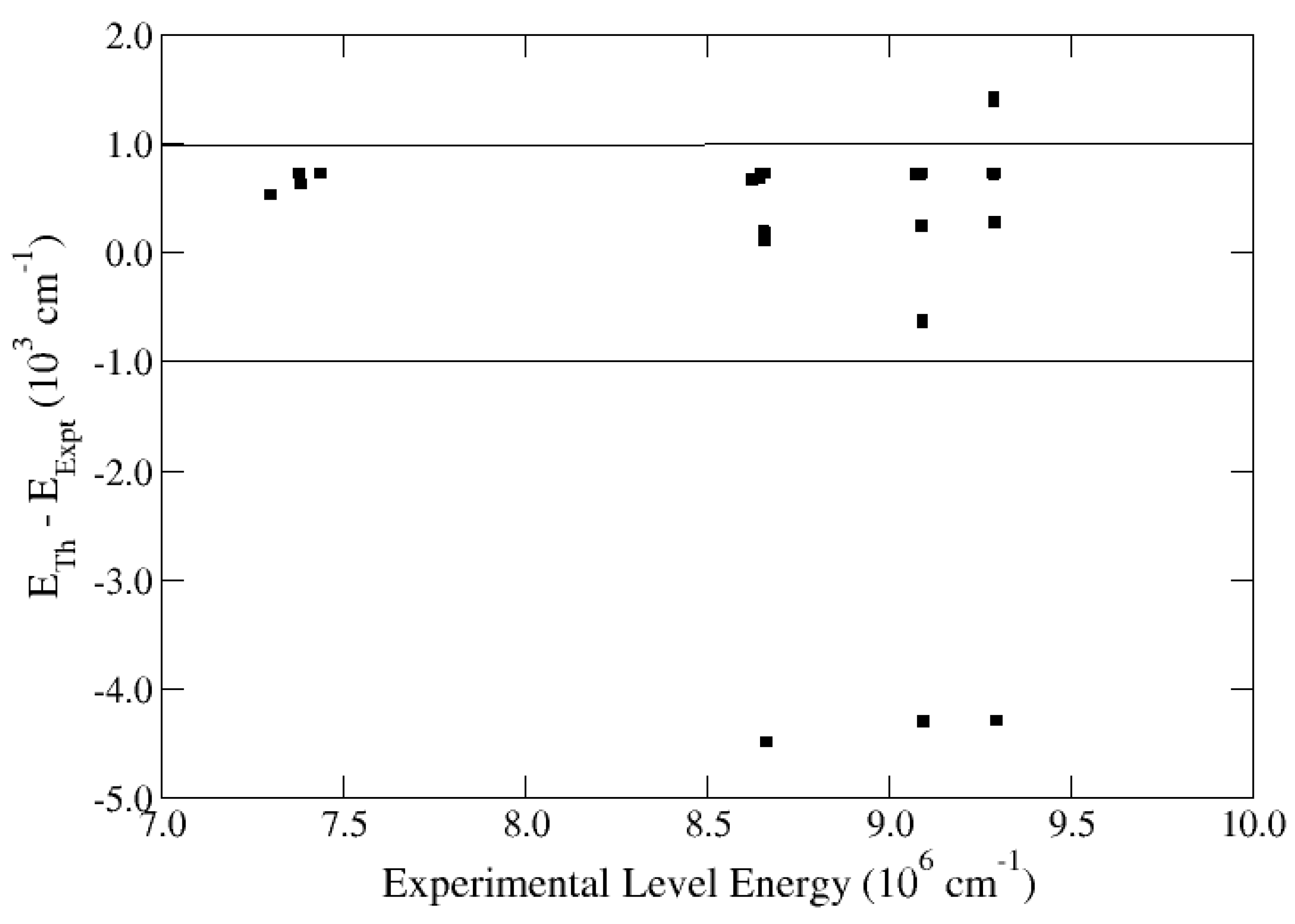As shown in Figure 5, the differences with theory for Ne ix are within the band $\text{Δ}E(10,2)=\pm 1000$ cm${}^{-1}$ except for six levels: $3{}^1{\mathrm{D}}_2$, $4{}^1{\mathrm{F}}_3^{\mathrm{o}}$, $5{}^3{\mathrm{D}}_J$ and $5{}^1{\mathrm{F}}_3^{\mathrm{o}}$, whose experimental energy positions could perhaps be due for a revision.

Figure 5. Level energy differences in Ne ix between the theoretical values of [121] and the experimental data listed in the nist database (v5.1). Such differences are mostly bound to the interval $\pm 1000$ cm${}^{-1}$ except for six levels whose spectroscopic positions are open for a revision.

Figure 5. Level energy differences in Ne ix between the theoretical values of [121] and the experimental data listed in the nist database (v5.1). Such differences are mostly bound to the interval $\pm 1000$ cm${}^{-1}$ except for six levels whose spectroscopic positions are open for a revision.

For E1 transitions, the $A{(6-8,2)}_{\mathrm{E}1}$ computed in [121] are within 0.7% of the standard except for $A{(7-8,2,n{}^1{\mathrm{P}}_1^{\mathrm{o}},n{}^1{\mathrm{D}}_2)}_{\mathrm{E}1}$ and $A{(7-8,2,n{}^3{\mathrm{D}}_{\mathrm{J}},n{}^3{\mathrm{P}}_{{\mathrm{J}}^{\prime }}^{\mathrm{o}})}_{\mathrm{E}1}$; that is, $\text{Δ}n=0$ transitions subject to the strong aforementioned cancellation effects. Furthermore, their $n=2$ forbidden transitions are also in good accord ($\lesssim 1$%) except for the sensitive intercombination transitions $A{(6-8,2,2{}^3{\mathrm{P}}_1^{\mathrm{o}},1{}^1{\mathrm{S}}_0)}_{\mathrm{E}1}$ that are $\lesssim 4$%. The most revealing comparison, in fact, is of the electric quadrupole rates $A{(Z,2,3-5{}^1{\mathrm{D}}_2,1{}^1{\mathrm{S}}_0)}_{\mathrm{E}2}$ computed by Savukov et al. [121] with those by Godefroid and Verhaegen [108] using the mchf method and Cann and Thakkar [112] by means of explicitly correlated wave functions. Apart from satisfactory agreement ($\lesssim 5$%), it brings out incorrect data for $A{(6-8,2,3{}^1{\mathrm{D}}_2,1{}^1{\mathrm{S}}_0)}_{\mathrm{E}2}$ in the nist database (v5.1); as indicated in the nist web page, the A-values by Cann and Thakkar [112] are listed for this transition for $2\le Z\le 5$ while those by Godefroid and Verhaegen [108] for $6\le Z\le 8$. However, as demonstrated in Table 4, the nist A-values for $6\le Z\le 8$ are low by a factor of 2/3, which appears to indicate the use of incorrect statistical weights in the conversion formula from $gf$-values to A-values; it may also be therein appreciated the excellent overall agreement that prevails among the theoretical data.

Table 4. Comparison of the $A(2-10,2,3{}^1{\mathrm{D}}_2,1{}^1{\mathrm{S}}_0)$ (s${}^{-1}$) electric quadrupole (E2) rate showing the incorrectly assigned data in the nist database (v5.1) for $6\le Z\le 8$. GV: [108] computed with the mchf method. CT: [112] using explicitly correlated functions. SJS: [121] computed with a relativistic CI method. Excellent agreement is otherwise found among the computed A-values. Wavelengths are determined from the nist level energies.

Z	λ (Å)	nist	gv	ct	sjs
2	5.3733E+02	1.2990E+03	1.293E+03	1.299E+03
3	1.7817E+02	8.2665E+04	8.254E+04	8.267E+04
4	8.8381E+01	9.2668E+05	9.253E+05	9.267E+05
5	5.2720E+01	5.1458E+06	5.139E+06	5.146E+06
6	3.4995E+01	1.2960E+07	1.944E+07	1.946E+07	1.936E+07
7	2.4914E+01	3.8470E+07	5.770E+07	5.775E+07	5.715E+07
8	1.8638E+01	9.6560E+07	1.448E+08	1.450E+08	1.423E+08

Table 4. Comparison of the $A(2-10,2,3{}^1{\mathrm{D}}_2,1{}^1{\mathrm{S}}_0)$ (s${}^{-1}$) electric quadrupole (E2) rate showing the incorrectly assigned data in the nist database (v5.1) for $6\le Z\le 8$. GV: [108] computed with the mchf method. CT: [112] using explicitly correlated functions. SJS: [121] computed with a relativistic CI method. Excellent agreement is otherwise found among the computed A-values. Wavelengths are determined from the nist level energies.

Z	λ (Å)	nist	gv	ct	sjs
2	5.3733E+02	1.2990E+03	1.293E+03	1.299E+03
3	1.7817E+02	8.2665E+04	8.254E+04	8.267E+04
4	8.8381E+01	9.2668E+05	9.253E+05	9.267E+05
5	5.2720E+01	5.1458E+06	5.139E+06	5.146E+06
6	3.4995E+01	1.2960E+07	1.944E+07	1.946E+07	1.936E+07
7	2.4914E+01	3.8470E+07	5.770E+07	5.775E+07	5.715E+07
8	1.8638E+01	9.6560E+07	1.448E+08	1.450E+08	1.423E+08

Table 5. Average differences (${10}^3$ cm${}^{-1}$) between the spectroscopic level energies of the nist database (v5.1) and those computed with grasp (${}^a$ [124], ${}^b$ [123], ${}^c$ [122], ${}^d$ [125]) and superstructure (^e [128], ${}^f$ [126], ${}^g$ [127]). grasp1: excludes Breit and QED effects. grasp2: includes Breit and QED effects. The quantity in brackets gives the standard error.

$\langle \text{Δ}E(Z,N)\rangle$	grasp1	grasp2	superstructure
$\langle \text{Δ}E(3,2)\rangle$	$-23.8\left(7\right)$ ${}^a$	$-23.9\left(7\right)$ ${}^a$
$\langle \text{Δ}E(4,2)\rangle$	$-23.0\left(8\right)$ ${}^a$	$-22.5\left(8\right)$ ${}^a$
$\langle \text{Δ}E(5,2)\rangle$	$-22.4\left(8\right)$ ${}^a$	$-22.9\left(8\right)$ ${}^a$
$\langle \text{Δ}E(6,2)\rangle$	$-21.9\left(8\right)$ ${}^a$	$-22.6\left(8\right)$ ${}^a$
$\langle \text{Δ}E(7,2)\rangle$	$-21.2\left(9\right)$ ${}^b$	$-22.5\left(9\right)$ ${}^b$	$+3.0\left(15\right)$ e
$\langle \text{Δ}E(8,2)\rangle$	$-20.1\left(9\right)$ ${}^c$	$-22.0\left(9\right)$ ${}^c$	$+0.79\left(53\right)$ ${}^f$
$\langle \text{Δ}E(9,2)\rangle$	$-20.6\left(15\right)$ ${}^b$	$-23.4\left(16\right)$ ${}^b$
$\langle \text{Δ}E(10,2)\rangle$	$+1.5\left(17\right)$ ${}^d$		$+5.0\left(20\right)$ e, $-3.5\left(17\right)$ ${}^g$

Table 5. Average differences (${10}^3$ cm${}^{-1}$) between the spectroscopic level energies of the nist database (v5.1) and those computed with grasp (${}^a$ [124], ${}^b$ [123], ${}^c$ [122], ${}^d$ [125]) and superstructure (^e [128], ${}^f$ [126], ${}^g$ [127]). grasp1: excludes Breit and QED effects. grasp2: includes Breit and QED effects. The quantity in brackets gives the standard error.

$\langle \text{Δ}E(Z,N)\rangle$	grasp1	grasp2	superstructure
$\langle \text{Δ}E(3,2)\rangle$	$-23.8\left(7\right)$ ${}^a$	$-23.9\left(7\right)$ ${}^a$
$\langle \text{Δ}E(4,2)\rangle$	$-23.0\left(8\right)$ ${}^a$	$-22.5\left(8\right)$ ${}^a$
$\langle \text{Δ}E(5,2)\rangle$	$-22.4\left(8\right)$ ${}^a$	$-22.9\left(8\right)$ ${}^a$
$\langle \text{Δ}E(6,2)\rangle$	$-21.9\left(8\right)$ ${}^a$	$-22.6\left(8\right)$ ${}^a$
$\langle \text{Δ}E(7,2)\rangle$	$-21.2\left(9\right)$ ${}^b$	$-22.5\left(9\right)$ ${}^b$	$+3.0\left(15\right)$ e
$\langle \text{Δ}E(8,2)\rangle$	$-20.1\left(9\right)$ ${}^c$	$-22.0\left(9\right)$ ${}^c$	$+0.79\left(53\right)$ ${}^f$
$\langle \text{Δ}E(9,2)\rangle$	$-20.6\left(15\right)$ ${}^b$	$-23.4\left(16\right)$ ${}^b$
$\langle \text{Δ}E(10,2)\rangle$	$+1.5\left(17\right)$ ${}^d$		$+5.0\left(20\right)$ e, $-3.5\left(17\right)$ ${}^g$

We now proceed to analyze the IC energy and radiative datasets obtained with structure codes: species $(3-9,2)$ [122,123,124] and $(10,2)$ [125] computed with grasp and $(7-8,2)$ [126,128] and $(10,2)$ [127,128] with superstructure, which are contained in the AtomPy zz_02 workbooks. In Table 5, we tabulate for these species the average differences between the spectroscopic level energies listed in the nist database (v5.1) and those obtained with grasp and superstructure; it must be noted that, for $(3-9,2)$, they have been calculated with and without the Breit and QED corrections. For $(3-9,2)$, the grasp average differences are approximately constant at $\langle \text{Δ}E(3-9,2)\rangle \sim -22\times {10}^3$ cm${}^{-1}$, and the inclusion of the Breit and QED corrections does not lead to significant reductions. By contrast, for $(10,2)$ the grasp average difference is an order of magnitude smaller ($1.5\times {10}^3$ cm${}^{-1}$) and so are those obtained with superstructure for other ions, a level of agreement more compatible with that encountered in the calculation by [121]. It must also be appreciated that, for $(10,2)$, the superstructure energy differences are both positive and negative depending on authorship. In conclusion, the general outcome of this exercise seems to indicate that a variety of strategies for atomic model optimization have been employed—some more successful than others—and due to their relevance in the final data products, a great deal of pondering and effort must go into the atomic system representation.

Moreover, we have found that only a fraction of the published A-values for He-like ions computed with grasp are in reasonable agreement (within 10%, say) with the standard and the accurate dataset by [121]. This fraction is $\sim 40$%–60% for E1 transitions and somewhat lower or similar for the forbidden transitions: $\sim 30$%–50% for E2 and M1 and $\sim 50$%–60% for M2, and it tends to increase slowly with Z. The A-values calculated in [127] for $(10,2)$ with superstructure are mainly for 17 strong E1 transitions ($logA>7$) that are found to be in good agreement (better than 10%) with the standard except for $A(10,2,3{}^1{\mathrm{P}}^{\mathrm{o}},1{}^1\mathrm{S})$.

Figure 6. Ratio of theoretical A-values for selected transitions relative to the standard [110,113]. (a) $A{(2-10,2,2{}^1{\mathrm{P}}^{\mathrm{o}},1{}^1\mathrm{S})}_{\mathrm{E}1}$; (b) $A{(2-10,2,2{}^3\mathrm{S},1{}^1\mathrm{S})}_{\mathrm{M}1}$ and (c) $A{(2-10,2,3{}^1\mathrm{D},1{}^1\mathrm{S})}_{\mathrm{E}2}$. Filled circles: calculations with grasp for $(3-9,2)$ [122,123,124]. Star: calculation with grasp for $(10,2)$ [125]. Squares: calculation with autostructure, present work. Crosses: relativistic CI calculation [121]. Diamonds: A-values from the norad database computed with the R-matrix method [95,119,120]. Triangles: OP [129].

Figure 6. Ratio of theoretical A-values for selected transitions relative to the standard [110,113]. (a) $A{(2-10,2,2{}^1{\mathrm{P}}^{\mathrm{o}},1{}^1\mathrm{S})}_{\mathrm{E}1}$; (b) $A{(2-10,2,2{}^3\mathrm{S},1{}^1\mathrm{S})}_{\mathrm{M}1}$ and (c) $A{(2-10,2,3{}^1\mathrm{D},1{}^1\mathrm{S})}_{\mathrm{E}2}$. Filled circles: calculations with grasp for $(3-9,2)$ [122,123,124]. Star: calculation with grasp for $(10,2)$ [125]. Squares: calculation with autostructure, present work. Crosses: relativistic CI calculation [121]. Diamonds: A-values from the norad database computed with the R-matrix method [95,119,120]. Triangles: OP [129].

In order to illustrate the problems in such datasets, we plot in Figure 6 the ratio relative to the standard [110,113] of A-values computed with different methods for three transitions along the isoelectronic sequence: the $A(2-10,2,2{}^1{\mathrm{P}}^{\mathrm{o}},1{}^1\mathrm{S})$ resonance (E1) transition, the $A(2-10,2,2{}^3\mathrm{S},1{}^1\mathrm{S})$ M1 transition within $n=2$ and the $A(2-10,2,3{}^1\mathrm{D},1{}^1\mathrm{S})$ E2 transition. For the E1 transition, it may be seen that, in comparison with the R-matrix (including OP) [95,119,120,129] and the relativistic CI method of [121], the data computed with grasp are noticeably higher ($\lesssim 20$%) for low Z, which seems to indicate insufficient correlation. We have also calculated A-values for the He-like ions $(2-10,2)$ with autostructure using atomic models containing the configurations

$$\{1{\mathrm{s}}^2,1\mathrm{s}2{\ell }_2,1\mathrm{s}3{\ell }_3,1\mathrm{s}4{\ell }_4,1\mathrm{s}5{\ell }_5\}$$

(4)

with $0\le {\ell }_n\le n-1$, and as shown in Figure 6a, for $A{(Z,2,2{}^1{\mathrm{P}}^{\mathrm{o}},1{}^1\mathrm{S})}_{\mathrm{E}1}$ they are not much different from those by grasp. More comparable values are obtained with autostructure for low Z by adopting the CI expansions of [108]:

$$\begin{array}{ccc}\hfill |1{}^1\mathrm{S}\rangle & =& \{n{\mathrm{s}}^2,n^{\prime }{\mathrm{p}}^2,n^{\prime \prime }{\mathrm{d}}^2,4{\mathrm{f}}^2,5{\mathrm{g}}^2\}\hfill \end{array}$$

(5)

$$\begin{array}{ccc}\hfill |2{}^1{\mathrm{P}}^{\mathrm{o}}\rangle & =& \{1\mathrm{s}2\mathrm{p},2\mathrm{s}3\mathrm{p},2\mathrm{p}3\mathrm{d},3\mathrm{d}4\mathrm{f}\}\hfill \end{array}$$

(6)

with $1\le n\le 4$, $2\le n^{\prime }\le 4$ and $3\le n^{″}\le 4$; however, the A-values are found to be very sensitive to the choice of the ${\lambda }_{1\mathrm{s}}$ scaling parameter of the statistical model potential used to generate the 1s orbital, not making it easy to arrive at an optimized value variationally. Single-excitation CI expansions of the type in Equation (4) have been extensively used for He-like targets in scattering calculations, while those in Equations (5) and (6), which include double excitations, would rapidly lead to unmanageable collisional targets. However, the quality of a collisional target is determined to a great extent by the accuracy of its radiative signatures; therefore, targets built up with poor CI expansions can lead to unreliable collision strengths. Furthermore, the situation with the M1 and E2 transitions in Figure 6b,c is not much different, i.e., distinctively discrepant A-values for low Z, but in this case autostructure performs somewhat better than grasp. Again, more accurate A-values for low Z can be obtained with autostructure with the double-excitation CI expansions [108]

$$\begin{array}{ccc}\hfill |2{}^3\mathrm{S}\rangle & =& \{1\mathrm{s}2\mathrm{s},3\mathrm{s}4\mathrm{s},2\mathrm{p}3\mathrm{p},4\mathrm{p}5\mathrm{p},3\mathrm{d}4\mathrm{d}\}\hfill \end{array}$$

(7)

$$\begin{array}{ccc}\hfill |3{}^1\mathrm{D}\rangle & =& \{1\mathrm{s}3\mathrm{d},2{\mathrm{p}}^2,3{\mathrm{p}}^2,3{\mathrm{d}}^2,2\mathrm{p}4\mathrm{f}\}.\hfill \end{array}$$

(8)

This unconverged correlation in He-like collisional targets becomes more acute for excited states as shown in Figure 7 where we plot $A{(Z,2,n{}^1{\mathrm{P}}^{\mathrm{o}},1{}^1\mathrm{S})}_{\mathrm{E}1}$ for $2\le n\le 9$ and $Z=6$ and $Z=10$. Firstly, there is excellent agreement between the OP A-values [129] and those obtained with the relativistic CI calculation of [121]. On the other hand, the differences with the data computed with grasp for C v [124] and Ne ix [125] are significant and grow with n; for C v, the relative difference between grasp and [121] for $n=5$ is a factor of three (see Figure 7). It may also be seen that A-values computed with autostrcuture show this similar discouraging behavior.

Figure 7. $A{(Z,2,n{}^1{\mathrm{P}}^{\mathrm{o}},1{}^1\mathrm{S})}_{\mathrm{E}1}$ as a function of n for (a) $Z=6$ and (b) $Z=10$. Circles: mcdf calculation with grasp for $Z=6$ [124]. Stars: mcdf calculation with grasp for $Z=10$ [125]. Squares: Breit–Pauli CI calculation with autostructure, present work. Crosses: relativistic CI calculation [121]. Triangles: OP [129].

Figure 7. $A{(Z,2,n{}^1{\mathrm{P}}^{\mathrm{o}},1{}^1\mathrm{S})}_{\mathrm{E}1}$ as a function of n for (a) $Z=6$ and (b) $Z=10$. Circles: mcdf calculation with grasp for $Z=6$ [124]. Stars: mcdf calculation with grasp for $Z=10$ [125]. Squares: Breit–Pauli CI calculation with autostructure, present work. Crosses: relativistic CI calculation [121]. Triangles: OP [129].

Table 6. Experimental and theoretical lifetimes (s) for states in He i. Experiment: ${}^a$ [133]; ${}^b$ [134]; ${}^c$ [135]; ${}^d$ [136]; ${}^e$ [137]; ${}^f$ [138]; ${}^g$ [139]; ${}^h$ [140]. Theory: ${}^i$ [88]; ${}^j$ [118]. Note: the quantity in brackets gives the experimental error.

$\tau (2,2,i)$	Experiment	Theory
$\tau (2,2,2{}^3{\mathrm{S}}_1)$	$7.87\left(51\right)\mathrm{E}+03$ ${}^a$	$7.862\mathrm{E}+03$ ${}^i$
$\tau (2,2,2{}^1{\mathrm{P}}_1^{\mathrm{o}})$	$5.60\left(14\right)\mathrm{E}-10$ ${}^b$	$5.553\mathrm{E}-10$ ${}^i$, $5.560\mathrm{E}-10$ ${}^j$
$\tau (2,2,3{}^3{\mathrm{S}}_1)$	$3.594\left(20\right)\mathrm{E}-08$ ${}^c$	$3.590\mathrm{E}-08$ ${}^i$, $3.588\mathrm{E}-08$ ${}^j$
$\tau (2,2,3{}^1{\mathrm{S}}_0)$	$5.63\left(20\right)\mathrm{E}-08$ ${}^d$	$5.465\mathrm{E}-08$ ${}^i$, $5.463\mathrm{E}-08$ ${}^j$
$\tau (2,2,3{}^3{\mathrm{P}}^{\mathrm{o}})$	$1.05\left(10\right)\mathrm{E}-07$ ${}^d$, $9.64\left(82\right)\mathrm{E}-08$ e	$9.480\mathrm{E}-08$ ${}^i$, $9.475\mathrm{E}-08$ ${}^j$
$\tau (2,2,3{}^3\mathrm{D})$	$1.412\left(6\right)\mathrm{E}-08$ ${}^c$, $1.42\left(6\right)\mathrm{E}-08$ ${}^f$	$1.414\mathrm{E}-08$ ${}^i$, $1.414\mathrm{E}-{08}^j$
$\tau (2,2,3{}^1{\mathrm{D}}_2)$	$1.53\left(3\right)\mathrm{E}-08$ ${}^f$	$1.569\mathrm{E}-08$ ${}^i$, $1.569\mathrm{E}-08$ ${}^j$
$\tau (2,2,3{}^1{\mathrm{P}}_1^{\mathrm{o}})$	$1.71\left(4\right)\mathrm{E}-09$ ${}^b$	$1.724\mathrm{E}-09$ ${}^i$, $1.725\mathrm{E}-09$ ${}^j$
$\tau (2,2,4{}^1{\mathrm{S}}_0)$	$8.87\left(30\right)\mathrm{E}-08$ ${}^d$	$8.800\mathrm{E}-08$ ${}^i$, $8.801\mathrm{E}-08$ ${}^j$
$\tau (2,2,4{}^3{\mathrm{P}}^{\mathrm{o}})$	$1.64\left(7\right)\mathrm{E}-07$ ${}^d$	$1.385\mathrm{E}-07$ ${}^i$, $1.385\mathrm{E}-07$ ${}^j$
$\tau (2,2,4{}^1{\mathrm{D}}_2)$	$3.1\left(3\right)\mathrm{E}-08$ ${}^g$	$3.707\mathrm{E}-08$ ${}^i$, $3.706\mathrm{E}-08$ ${}^j$
$\tau (2,2,4{}^1{\mathrm{F}}_3^{\mathrm{o}})$	$7.4\left(2\right)\mathrm{E}-08$ ${}^h$	$7.229\mathrm{E}-08$ ${}^i$
$\tau (2,2,4{}^1{\mathrm{P}}_1^{\mathrm{o}})$	$4.01\left(8\right)\mathrm{E}-09$ ${}^b$, $4.3\left(2\right)\mathrm{E}-09$ ${}^g$	$3.964\mathrm{E}-09$ ${}^i$, $3.967\mathrm{E}-09$ ${}^j$
$\tau (2,2,5{}^1{\mathrm{S}}_0)$	$1.49\left(5\right)\mathrm{E}-07$ ${}^d$	$1.465\mathrm{E}-07$ ${}^i$, $1.466\mathrm{E}-07$ ${}^j$
$\tau (2,2,5{}^3{\mathrm{P}}^{\mathrm{o}})$	$2.45\left(15\right)\mathrm{E}-07$ ${}^d$	$2.193\mathrm{E}-07$ ${}^i$, $2.193\mathrm{E}-07$ ${}^j$
$\tau (2,2,5{}^1{\mathrm{D}}_2)$	$5.4\left(5\right)\mathrm{E}-08$ ${}^g$	$7.180\mathrm{E}-08$ ${}^i$, $7.205\mathrm{E}-08$ ${}^j$
$\tau (2,2,5{}^1{\mathrm{F}}_3^{\mathrm{o}})$	$1.33\left(5\right)\mathrm{E}-07$ ${}^h$	$1.398\mathrm{E}-07$ ${}^i$
$\tau (2,2,5{}^1{\mathrm{P}}_1^{\mathrm{o}})$	$7.68\left(15\right)\mathrm{E}-09$ ${}^b$	$7.625\mathrm{E}-09$ ${}^i$, $7.631\mathrm{E}-09$ ${}^j$

Table 6. Experimental and theoretical lifetimes (s) for states in He i. Experiment: ${}^a$ [133]; ${}^b$ [134]; ${}^c$ [135]; ${}^d$ [136]; ${}^e$ [137]; ${}^f$ [138]; ${}^g$ [139]; ${}^h$ [140]. Theory: ${}^i$ [88]; ${}^j$ [118]. Note: the quantity in brackets gives the experimental error.

$\tau (2,2,i)$	Experiment	Theory
$\tau (2,2,2{}^3{\mathrm{S}}_1)$	$7.87\left(51\right)\mathrm{E}+03$ ${}^a$	$7.862\mathrm{E}+03$ ${}^i$
$\tau (2,2,2{}^1{\mathrm{P}}_1^{\mathrm{o}})$	$5.60\left(14\right)\mathrm{E}-10$ ${}^b$	$5.553\mathrm{E}-10$ ${}^i$, $5.560\mathrm{E}-10$ ${}^j$
$\tau (2,2,3{}^3{\mathrm{S}}_1)$	$3.594\left(20\right)\mathrm{E}-08$ ${}^c$	$3.590\mathrm{E}-08$ ${}^i$, $3.588\mathrm{E}-08$ ${}^j$
$\tau (2,2,3{}^1{\mathrm{S}}_0)$	$5.63\left(20\right)\mathrm{E}-08$ ${}^d$	$5.465\mathrm{E}-08$ ${}^i$, $5.463\mathrm{E}-08$ ${}^j$
$\tau (2,2,3{}^3{\mathrm{P}}^{\mathrm{o}})$	$1.05\left(10\right)\mathrm{E}-07$ ${}^d$, $9.64\left(82\right)\mathrm{E}-08$ e	$9.480\mathrm{E}-08$ ${}^i$, $9.475\mathrm{E}-08$ ${}^j$
$\tau (2,2,3{}^3\mathrm{D})$	$1.412\left(6\right)\mathrm{E}-08$ ${}^c$, $1.42\left(6\right)\mathrm{E}-08$ ${}^f$	$1.414\mathrm{E}-08$ ${}^i$, $1.414\mathrm{E}-{08}^j$
$\tau (2,2,3{}^1{\mathrm{D}}_2)$	$1.53\left(3\right)\mathrm{E}-08$ ${}^f$	$1.569\mathrm{E}-08$ ${}^i$, $1.569\mathrm{E}-08$ ${}^j$
$\tau (2,2,3{}^1{\mathrm{P}}_1^{\mathrm{o}})$	$1.71\left(4\right)\mathrm{E}-09$ ${}^b$	$1.724\mathrm{E}-09$ ${}^i$, $1.725\mathrm{E}-09$ ${}^j$
$\tau (2,2,4{}^1{\mathrm{S}}_0)$	$8.87\left(30\right)\mathrm{E}-08$ ${}^d$	$8.800\mathrm{E}-08$ ${}^i$, $8.801\mathrm{E}-08$ ${}^j$
$\tau (2,2,4{}^3{\mathrm{P}}^{\mathrm{o}})$	$1.64\left(7\right)\mathrm{E}-07$ ${}^d$	$1.385\mathrm{E}-07$ ${}^i$, $1.385\mathrm{E}-07$ ${}^j$
$\tau (2,2,4{}^1{\mathrm{D}}_2)$	$3.1\left(3\right)\mathrm{E}-08$ ${}^g$	$3.707\mathrm{E}-08$ ${}^i$, $3.706\mathrm{E}-08$ ${}^j$
$\tau (2,2,4{}^1{\mathrm{F}}_3^{\mathrm{o}})$	$7.4\left(2\right)\mathrm{E}-08$ ${}^h$	$7.229\mathrm{E}-08$ ${}^i$
$\tau (2,2,4{}^1{\mathrm{P}}_1^{\mathrm{o}})$	$4.01\left(8\right)\mathrm{E}-09$ ${}^b$, $4.3\left(2\right)\mathrm{E}-09$ ${}^g$	$3.964\mathrm{E}-09$ ${}^i$, $3.967\mathrm{E}-09$ ${}^j$
$\tau (2,2,5{}^1{\mathrm{S}}_0)$	$1.49\left(5\right)\mathrm{E}-07$ ${}^d$	$1.465\mathrm{E}-07$ ${}^i$, $1.466\mathrm{E}-07$ ${}^j$
$\tau (2,2,5{}^3{\mathrm{P}}^{\mathrm{o}})$	$2.45\left(15\right)\mathrm{E}-07$ ${}^d$	$2.193\mathrm{E}-07$ ${}^i$, $2.193\mathrm{E}-07$ ${}^j$
$\tau (2,2,5{}^1{\mathrm{D}}_2)$	$5.4\left(5\right)\mathrm{E}-08$ ${}^g$	$7.180\mathrm{E}-08$ ${}^i$, $7.205\mathrm{E}-08$ ${}^j$
$\tau (2,2,5{}^1{\mathrm{F}}_3^{\mathrm{o}})$	$1.33\left(5\right)\mathrm{E}-07$ ${}^h$	$1.398\mathrm{E}-07$ ${}^i$
$\tau (2,2,5{}^1{\mathrm{P}}_1^{\mathrm{o}})$	$7.68\left(15\right)\mathrm{E}-09$ ${}^b$	$7.625\mathrm{E}-09$ ${}^i$, $7.631\mathrm{E}-09$ ${}^j$

Table 7. Experimental and theoretical lifetimes (s) for states in He-like ions. ${}^a$ [141]; ${}^b$ [132]; ${}^c$ [142]; ${}^d$ [143]; ${}^e$ [144]; ${}^f$ [145]; ${}^g$ [146]; ${}^h$ [147]; ${}^i$ [148]. Theory: ${}^j$ [88]; ${}^k$ [149]; ${}^l$ [150]; ${}^m$ [121]; ${}^n$ [105]. Note: the quantity in brackets gives the experimental error.

$\tau (Z,2,i)$	Experiment	Theory
$\tau (3,2,2{}^3{\mathrm{S}}_1)$	$5.22\left(50\right)\mathrm{E}+01$ ${}^a$	$4.904\mathrm{E}+01$ ${}^j$
$\tau (4,2,2{}^3{\mathrm{S}}_1)$	$1.80\left(5\right)\mathrm{E}+00$ ${}^b$	$1.780\mathrm{E}+00$ ${}^k$
$\tau (4,2,2{}^3{\mathrm{P}}_2^{\mathrm{o}})$	$2.91\left(2\right)\mathrm{E}-08$ ${}^c$	$2.934\mathrm{E}-08$ ${}^k$
$\tau (6,2,2{}^3{\mathrm{S}}_1)$	$2.059\left(5\right)\mathrm{E}-02$ ${}^d$	$2.059\mathrm{E}-02$ ${}^l$, $2.052\mathrm{E}-02$ ${}^m$
$\tau (6,2,2{}^3{\mathrm{P}}_1^{\mathrm{o}})$	$1.13\left(5\right)\mathrm{E}-08$ e	$1.185\mathrm{E}-08$ ${}^l$, $1.195\mathrm{E}-08$ ${}^m$
$\tau (6,2,2{}^3{\mathrm{P}}_2^{\mathrm{o}})$	$1.67\left(6\right)\mathrm{E}-08$ e	$1.763\mathrm{E}-08$ ${}^l$, $1.747\mathrm{E}-08$ ${}^m$
$\tau (7,2,2{}^3{\mathrm{S}}_1)$	$3.94\left(5\right)\mathrm{E}-03$ ${}^f$	$3.922\mathrm{E}-03$ ${}^l$, $3.932\mathrm{E}-03$ ${}^m$
$\tau (7,2,2{}^3{\mathrm{P}}_1^{\mathrm{o}})$	$4.9\left(3\right)\mathrm{E}-09$ e	$4.931\mathrm{E}-09$ ${}^m$
$\tau (7,2,2{}^3{\mathrm{P}}_2^{\mathrm{o}})$	$1.49\left(7\right)\mathrm{E}-08$ e	$1.463\mathrm{E}-08$ ${}^l$, $1.444\mathrm{E}-08$ ${}^m$
$\tau (8,2,2{}^3{\mathrm{S}}_1)$	$9.56\left(5\right)\mathrm{E}-04$ ${}^g$	$9.615\mathrm{E}-04$ ${}^l$, $9.551\mathrm{E}-04$ ${}^m$
$\tau (8,2,2{}^3{\mathrm{P}}_1^{\mathrm{o}})$	$1.52\left(8\right)\mathrm{E}-09$ ${}^h$	$1.625\mathrm{E}-09$ ${}^m$
$\tau (8,2,2{}^3{\mathrm{P}}_2^{\mathrm{o}})$	$1.210\left(20\right)\mathrm{E}-08$ ${}^h$	$1.240\mathrm{E}-08$ ${}^l$, $1.216\mathrm{E}-08$ ${}^m$
$\tau (9,2,2{}^3{\mathrm{S}}_1)$	$2.76\left(2\right)\mathrm{E}-04$ ${}^f$	$2.772\mathrm{E}-04$ ${}^n$
$\tau (9,2,2{}^3{\mathrm{P}}_1^{\mathrm{o}})$	$5.31\left(20\right)\mathrm{E}-10$ ${}^h$
$\tau (9,2,2{}^3{\mathrm{P}}_2^{\mathrm{o}})$	$1.044\left(15\right)\mathrm{E}-08$ ${}^h$
$\tau (10,2,2{}^3{\mathrm{S}}_1)$	$9.17\left(4\right)\mathrm{E}-05$ ${}^i$	$9.141\mathrm{E}-05$ ${}^m$, $9.200\mathrm{E}-05$ ${}^n$

Table 7. Experimental and theoretical lifetimes (s) for states in He-like ions. ${}^a$ [141]; ${}^b$ [132]; ${}^c$ [142]; ${}^d$ [143]; ${}^e$ [144]; ${}^f$ [145]; ${}^g$ [146]; ${}^h$ [147]; ${}^i$ [148]. Theory: ${}^j$ [88]; ${}^k$ [149]; ${}^l$ [150]; ${}^m$ [121]; ${}^n$ [105]. Note: the quantity in brackets gives the experimental error.

$\tau (Z,2,i)$	Experiment	Theory
$\tau (3,2,2{}^3{\mathrm{S}}_1)$	$5.22\left(50\right)\mathrm{E}+01$ ${}^a$	$4.904\mathrm{E}+01$ ${}^j$
$\tau (4,2,2{}^3{\mathrm{S}}_1)$	$1.80\left(5\right)\mathrm{E}+00$ ${}^b$	$1.780\mathrm{E}+00$ ${}^k$
$\tau (4,2,2{}^3{\mathrm{P}}_2^{\mathrm{o}})$	$2.91\left(2\right)\mathrm{E}-08$ ${}^c$	$2.934\mathrm{E}-08$ ${}^k$
$\tau (6,2,2{}^3{\mathrm{S}}_1)$	$2.059\left(5\right)\mathrm{E}-02$ ${}^d$	$2.059\mathrm{E}-02$ ${}^l$, $2.052\mathrm{E}-02$ ${}^m$
$\tau (6,2,2{}^3{\mathrm{P}}_1^{\mathrm{o}})$	$1.13\left(5\right)\mathrm{E}-08$ e	$1.185\mathrm{E}-08$ ${}^l$, $1.195\mathrm{E}-08$ ${}^m$
$\tau (6,2,2{}^3{\mathrm{P}}_2^{\mathrm{o}})$	$1.67\left(6\right)\mathrm{E}-08$ e	$1.763\mathrm{E}-08$ ${}^l$, $1.747\mathrm{E}-08$ ${}^m$
$\tau (7,2,2{}^3{\mathrm{S}}_1)$	$3.94\left(5\right)\mathrm{E}-03$ ${}^f$	$3.922\mathrm{E}-03$ ${}^l$, $3.932\mathrm{E}-03$ ${}^m$
$\tau (7,2,2{}^3{\mathrm{P}}_1^{\mathrm{o}})$	$4.9\left(3\right)\mathrm{E}-09$ e	$4.931\mathrm{E}-09$ ${}^m$
$\tau (7,2,2{}^3{\mathrm{P}}_2^{\mathrm{o}})$	$1.49\left(7\right)\mathrm{E}-08$ e	$1.463\mathrm{E}-08$ ${}^l$, $1.444\mathrm{E}-08$ ${}^m$
$\tau (8,2,2{}^3{\mathrm{S}}_1)$	$9.56\left(5\right)\mathrm{E}-04$ ${}^g$	$9.615\mathrm{E}-04$ ${}^l$, $9.551\mathrm{E}-04$ ${}^m$
$\tau (8,2,2{}^3{\mathrm{P}}_1^{\mathrm{o}})$	$1.52\left(8\right)\mathrm{E}-09$ ${}^h$	$1.625\mathrm{E}-09$ ${}^m$
$\tau (8,2,2{}^3{\mathrm{P}}_2^{\mathrm{o}})$	$1.210\left(20\right)\mathrm{E}-08$ ${}^h$	$1.240\mathrm{E}-08$ ${}^l$, $1.216\mathrm{E}-08$ ${}^m$
$\tau (9,2,2{}^3{\mathrm{S}}_1)$	$2.76\left(2\right)\mathrm{E}-04$ ${}^f$	$2.772\mathrm{E}-04$ ${}^n$
$\tau (9,2,2{}^3{\mathrm{P}}_1^{\mathrm{o}})$	$5.31\left(20\right)\mathrm{E}-10$ ${}^h$
$\tau (9,2,2{}^3{\mathrm{P}}_2^{\mathrm{o}})$	$1.044\left(15\right)\mathrm{E}-08$ ${}^h$
$\tau (10,2,2{}^3{\mathrm{S}}_1)$	$9.17\left(4\right)\mathrm{E}-05$ ${}^i$	$9.141\mathrm{E}-05$ ${}^m$, $9.200\mathrm{E}-05$ ${}^n$

Table 8. Experimental and theoretical transition rates (s${}^{-1}$) for He-like ions. ${}^a$ [151]; ${}^b$ [152]; ${}^c$ [153]; ${}^d$ [154]; ${}^e$ [144]; ${}^f$ [147]. Theory: ${}^g$ [88]; ${}^h$ [118]; ${}^i$ [107]; ${}^j$ [121]. Note: the quantity in brackets gives the experimental error.

$A(Z,2,k,i)$	Experiment	Theory
$A(2,2,2{}^3{\mathrm{P}}_1^{\mathrm{o}},1{}^1{\mathrm{S}}_0)$	$1.77\left(8\right)\mathrm{E}+{02}^a$	$1.764\mathrm{E}+{02}^g$, $1.731\mathrm{E}+{02}^h$
$A(2,2,2{}^3{\mathrm{P}}_2^{\mathrm{o}},1{}^1{\mathrm{S}}_0)$	$3.24\left(16\right)\mathrm{E}-{01}^b$	$3.270\mathrm{E}-{01}^g$
$A(2,2,2{}^1{\mathrm{P}}_1^{\mathrm{o}},1{}^1{\mathrm{S}}_0)$	$1.758\left(50\right)\mathrm{E}+{09}^c$, $1.82\left(5\right)\mathrm{E}+{09}^d$	$1.799\mathrm{E}+{09}^g$, $1.797\mathrm{E}+{09}^h$
$A(2,2,3{}^1{\mathrm{P}}_1^{\mathrm{o}},1{}^1{\mathrm{S}}_0)$	$5.68\left(18\right)\mathrm{E}+{08}^c$, $5.71\left(5\right)\mathrm{E}+{08}^d$	$5.663\mathrm{E}+{08}^g$, $5.660\mathrm{E}+{08}^h$
$A(2,2,4{}^1{\mathrm{P}}_1^{\mathrm{o}},1{}^1{\mathrm{S}}_0)$	$2.47\left(6\right)\mathrm{E}+{08}^d$	$2.436\mathrm{E}+{08}^g$, $2.434\mathrm{E}+{08}^h$
$A(2,2,5{}^1{\mathrm{P}}_1^{\mathrm{o}},1{}^1{\mathrm{S}}_0)$	$1.27\left(3\right)\mathrm{E}+{08}^d$	$1.258\mathrm{E}+{08}^g$, $1.257\mathrm{E}+{08}^h$
$A(6,2,2{}^3{\mathrm{P}}_1^{\mathrm{o}},1{}^1{\mathrm{S}}_0)$	$2.90\left(16\right)\mathrm{E}+{07}^e$	$2.825\mathrm{E}+{07}^i$, $2.701\mathrm{E}+{07}^j$
$A(7,2,2{}^3{\mathrm{P}}_1^{\mathrm{o}},1{}^1{\mathrm{S}}_0)$	$1.38\left(11\right)\mathrm{E}+{08}^e$	$1.394\mathrm{E}+{08}^i$, $1.348\mathrm{E}+{08}^j$
$A(8,2,2{}^3{\mathrm{P}}_1^{\mathrm{o}},1{}^1{\mathrm{S}}_0)$	$5.80\left(35\right)\mathrm{E}+{08}^f$	$5.499\mathrm{E}+{08}^i$, $5.357\mathrm{E}+{08}^j$
$A(9,2,2{}^3{\mathrm{P}}_1^{\mathrm{o}},1{}^1{\mathrm{S}}_0)$	$1.78\left(7\right)\mathrm{E}+{09}^f$	$1.834\mathrm{E}+{09}^i$

Table 8. Experimental and theoretical transition rates (s${}^{-1}$) for He-like ions. ${}^a$ [151]; ${}^b$ [152]; ${}^c$ [153]; ${}^d$ [154]; ${}^e$ [144]; ${}^f$ [147]. Theory: ${}^g$ [88]; ${}^h$ [118]; ${}^i$ [107]; ${}^j$ [121]. Note: the quantity in brackets gives the experimental error.

$A(Z,2,k,i)$	Experiment	Theory
$A(2,2,2{}^3{\mathrm{P}}_1^{\mathrm{o}},1{}^1{\mathrm{S}}_0)$	$1.77\left(8\right)\mathrm{E}+{02}^a$	$1.764\mathrm{E}+{02}^g$, $1.731\mathrm{E}+{02}^h$
$A(2,2,2{}^3{\mathrm{P}}_2^{\mathrm{o}},1{}^1{\mathrm{S}}_0)$	$3.24\left(16\right)\mathrm{E}-{01}^b$	$3.270\mathrm{E}-{01}^g$
$A(2,2,2{}^1{\mathrm{P}}_1^{\mathrm{o}},1{}^1{\mathrm{S}}_0)$	$1.758\left(50\right)\mathrm{E}+{09}^c$, $1.82\left(5\right)\mathrm{E}+{09}^d$	$1.799\mathrm{E}+{09}^g$, $1.797\mathrm{E}+{09}^h$
$A(2,2,3{}^1{\mathrm{P}}_1^{\mathrm{o}},1{}^1{\mathrm{S}}_0)$	$5.68\left(18\right)\mathrm{E}+{08}^c$, $5.71\left(5\right)\mathrm{E}+{08}^d$	$5.663\mathrm{E}+{08}^g$, $5.660\mathrm{E}+{08}^h$
$A(2,2,4{}^1{\mathrm{P}}_1^{\mathrm{o}},1{}^1{\mathrm{S}}_0)$	$2.47\left(6\right)\mathrm{E}+{08}^d$	$2.436\mathrm{E}+{08}^g$, $2.434\mathrm{E}+{08}^h$
$A(2,2,5{}^1{\mathrm{P}}_1^{\mathrm{o}},1{}^1{\mathrm{S}}_0)$	$1.27\left(3\right)\mathrm{E}+{08}^d$	$1.258\mathrm{E}+{08}^g$, $1.257\mathrm{E}+{08}^h$
$A(6,2,2{}^3{\mathrm{P}}_1^{\mathrm{o}},1{}^1{\mathrm{S}}_0)$	$2.90\left(16\right)\mathrm{E}+{07}^e$	$2.825\mathrm{E}+{07}^i$, $2.701\mathrm{E}+{07}^j$
$A(7,2,2{}^3{\mathrm{P}}_1^{\mathrm{o}},1{}^1{\mathrm{S}}_0)$	$1.38\left(11\right)\mathrm{E}+{08}^e$	$1.394\mathrm{E}+{08}^i$, $1.348\mathrm{E}+{08}^j$
$A(8,2,2{}^3{\mathrm{P}}_1^{\mathrm{o}},1{}^1{\mathrm{S}}_0)$	$5.80\left(35\right)\mathrm{E}+{08}^f$	$5.499\mathrm{E}+{08}^i$, $5.357\mathrm{E}+{08}^j$
$A(9,2,2{}^3{\mathrm{P}}_1^{\mathrm{o}},1{}^1{\mathrm{S}}_0)$	$1.78\left(7\right)\mathrm{E}+{09}^f$	$1.834\mathrm{E}+{09}^i$

There have been extensive measurements of level lifetimes in He-like ions which, taking advantage of the high accuracy of the theoretical data, have led to useful benchmarks and progressive refinement of a variety of experimental methods. In Table 6 and Table 7 we give a representative but by no means exhaustive comparison between experiment and theory for $(2-10,2)$. It may be appreciated that the portfolio for He i includes excited states with $n\le 5$ while for $Z>2$ it is limited to $n=2$, but in most cases the theoretical lifetimes lie within the experimental error bars. Outstanding agreement (better than 1%) is found for $\tau (2,2,2-5{}^1{\mathrm{P}}_1^{\mathrm{o}})$ and $\tau (2-10,2,2{}^3{\mathrm{S}}_1)$, except for $Z=3$ where it deteriorates to $\sim 6$% due to experimental limitations of the heavy-ion storage ring [132]. The accord for $\tau (6-9,2,2{}^3{\mathrm{P}}_1^{\mathrm{o}})$ and $\tau (4-9,2,2{}^3{\mathrm{P}}_2^{\mathrm{o}})$ is found to be within 5%.

As shown in Table 8, measurements have also been reported for the transition rates $A{(2-9,2,2{}^3{\mathrm{P}}_1^{\mathrm{o}},1{}^1{\mathrm{S}}_0)}_{E1}$ and $A{(2,2,2-5{}^1{\mathrm{P}}_1^{\mathrm{o}},1{}^1{\mathrm{S}}_0)}_{E1}$, where the agreement with theory is within 3% except for $A{(8,2,2{}^3{\mathrm{P}}_1^{\mathrm{o}},1{}^1{\mathrm{S}}_0)}_{E1}$.

6. Conclusions and Recommendations

In the present work we have made an attempt to bring out and discuss new scientific research directions that are driven by collaborative data-intensive projects, and in this context, some of the problems that compromise reliable atomic data assessments for the astrophysical community. We have thus proposed a new scheme based on an open virtual research community of both atomic data producers and users to be engaged in an ongoing data-curation pursuit where data quality will be the prevalent currency. For this purpose we have developed a working prototype of a cloud-computing data curation environment on Google Drive, referred to as AtomPy, to promote the use, reuse, assessment and preservation of the atomic datasets. AtomPy is based on the powerful functionalities of Google Sheets and Pandas DataFrames, and opens a door to the GitHub social network for the development and sharing of atomic data manipulation workflows and Python utilities. The concept and possibilities of the workflow representation as the blueprint of a research process is innovative and is likely to play a major role in data-intensive science, and among the many workflow tools that are becoming available and after the experience of the present work, we recommend the use of IPython Notebooks.

With the aid of AtomPy we have proceeded to review the energy structures and radiative rates of ions in the hydrogen and helium isoelectronic sequences with atomic number $Z\le 10$, which has been an interesting opportunity to gauge the accuracy level that can be actually attained with the main body of the atomic computational codes, among them superstructure, autostructure, grasp, mchf, civ3 and R-matrix. As a result, we intend to denote our recommended datasets in the AtomPy metadata by upgrading their source identifications from Sn to Rn where n is just an integer assignment.

The critical compilations of radiative rates for isonuclear sequences with $Z\le 5$ [88,149] have prepared the stage for the present dataset comparisons by establishing the standard references for the H [100,101] and He [105,107,108,109,110,111,112,113,114,115,116] sequences. For the H sequence, we find that the A-values for allowed (E1) and forbidden (E2, E3, M1, M2, M3) transitions computed with grasp [97,98] are highly accurate (a few parts in ${10}^4$), the larger differences being among the magnetic dipole (M1) transitions with small line strengths. The relativistic A-values for E1 transitions in selected H-like ions of [102] also display this accuracy ranking. On the other hand, the A-values listed in the norad database for this sequence and computed with superstructure [90,91,92,93,94,95,96] are found to be accurate ($\sim 1$%) for E1 and E2 transitions, but large unexpected discrepancies appear for some E3, M1 and M2 transitions probably due to computer bugs.

Regarding the He isoelectronic sequence, we have found that in general the E1 A-values calculated with the R-matrix method for the neutral and higher members—in both $LS$ [90,95,119,120] and intermediate [118] couplings and involving highly excited states ($n\le 10$)—are of satisfactory accuracy. We should also include in this ranked group the older rates from the OP [129], which reinforce the longstanding effectiveness of the R-matrix method for the computation of large and accurate radiative datasets for allowed transitions; furthermore, taking into account the impressive accuracy reached in the IC data for He I [118] with a variation of this method, it can certainly be extended to the more sensitive intercombination ($\text{Δ}S\ne 0$) transitions.

We also find that the energies and radiative rates for E1, E2, M1 and M2 transitions in selected He-like ions computed in a fully relativistic CI approach [121] are of outstanding accuracy (A-values better than 1%), and have allowed us to evaluate the consistency of other energy and radiative datasets, including some of the nist database: some inaccurate E2 A-values and curable spectroscopic level energies in Ne ix.

Most of the radiative datasets that have been computed with grasp [122,123,124,125] and superstructure [127] (A-values from [126,128] were not available) for He-like ions have used CI expansions streamlined for collisional targets rather than to obtain accurate A-values. Therefore, such CI is not fully converged, and the accuracy for both allowed and forbidden transitions in low-Z ions and involving excited states can be poor. In the case of the datasets computed with grasp, just over a half of the A-values are within 10% of the standard, particularly discrepant transitions being those in the principal series and E2 in ions with $Z\le 8$. The situation is not that critical in the A-values for Ne ix listed in [127] as only strong E1, low-n transitions were considered.

We have carried out a fairly extensive comparison of experimental and theoretical lifetimes for He-like ions that brings out two important points. Firstly, the high degree of experimental precision for metastables, e.g., $\tau (Z,2,2{}^3\mathrm{S})$, and the excellent agreement with theoretical estimates have thoroughly validated the finer grain of radiation theory (e.g., Breit M1 corrections). Secondly, the quality of theoretical radiative rates for He-like ions has been useful to benchmark a wide variety of experimental techniques that intend to focus excited states and states with much shorter lifetimes.

We would like to close this review by recalling that the datasets that have been analyzed in the present work are openly available from AtomPy [67], and by making a plea to data producers regarding publishing formats. The latter do not often facilitate machine reading or even manual transcriptions and, consequently, become a burden for compilations and sound curation. A general effort to make the atomic data available at least in digital format would indeed be welcome.

References

1. Hey, T.; Trefethen, A.E. Cyberinfrastructure for e-Science. Science 2005, 308, 817–821. [Google Scholar] [CrossRef] [PubMed]
2. Seaton, M.J. The Opacity Project; Institute of Physics Publishing: Bristol, UK, 1995. [Google Scholar]
3. Available online: http://cdsweb.u-strasbg.fr/topbase/testop/TheOP.html (accessed on 28 April 2014).
4. Hummer, D.G.; Berrington, K.A.; Eissner, W.; Pradhan, A.K.; Saraph, H.E.; Tully, J.A. Atomic data from the IRON Project. 1: Goals and methods. Astron. Astrophys. 1993, 279, 298–309. [Google Scholar]
5. Available online: http://cdsweb.u-strasbg.fr/topbase/testop/TheIP.html (accessed on 28 April 2014).
6. Berrington, K. Summary of the Iron and Opacity Projects. In Astrophysical Applications of Powerful New Databases; Adelman, S.J., Wiese, W.L., Eds.; Astronomical Society of the Pacific: San Francisco, CA, USA, 1995; Volume 78, ASP Conference Series; pp. 19–30. [Google Scholar]
7. Available online: http://cdsweb.u-strasbg.fr/topbase/topbase.html (accessed on 28 April 2014).
8. Cunto, W.; Mendoza, C. The Opacity Project—The Topbase atomic database. Rev. Mex. Astron. Astrofís. 1992, 23, 107–118. [Google Scholar]
9. Cunto, W.; Mendoza, C.; Ochsenbein, F.; Zeippen, C.J. Topbase at the CDS. Astron. Astrophys. 1993, 275, L5–L8. [Google Scholar]
10. Available online: http://cdsweb.u-strasbg.fr/tipbase/home.html (accessed on 28 April 2014).
11. Available online: http://opacities.osc.edu/ (accessed on 28 April 2014).
12. Mendoza, C.; Seaton, M.J.; Buerger, P.; Bellorín, A.; Meléndez, M.; González, J.; Rodríguez, L.S.; Delahaye, F.; Palacios, E.; Pradhan, A.K.; et al. OPserver: Interactive online computations of opacities and radiative accelerations. Mon. Not. R. Astron. Soc. 2007, 378, 1031–1035. [Google Scholar] [CrossRef]
13. Bell, G.; Hey, T.; Szalay, A. Beyond the data deluge. Science 2009, 323, 1297–1298. [Google Scholar] [CrossRef] [PubMed]
14. The Fourth Paradigm: Data-Intensive Scientific Discovery; Hey, T.; Tansley, S.; Tolle, K.M. (Eds.) Microsoft Research: Redmont, DC, USA, 2009.
15. Critchlow, T.; van Dam, K.K. Data-Intensive Science; Chapman and Hall/CRC Computational Science Series; CRC Press: Boca Raton, FL, USA, 2013. [Google Scholar]
16. Available online: http://physics.nist.gov/asd (accessed on 28 April 2014).
17. Kramida, A.; Ralchenko, Yu.; Reader, J.; NIST ASD Team. NIST Atomic Spectra Database (v5.1); National Institute of Standards and Technology: Gaithersburg, MD, USA, 2013. [Google Scholar]
18. Available online: http://www.chiantidatabase.org/ (accessed on 28 April 2014).
19. Dere, K.P.; Landi, E.; Mason, H.E.; Monsignori Fossi, B.C.; Young, P.R. CHIANTI—An atomic database for emission lines. Astron. Astrophys. Suppl. Ser. 1997, 125, 149–173. [Google Scholar] [CrossRef]
20. Landi, E.; Young, P.R.; Dere, K.P.; Del Zanna, G.; Mason, H.E. CHIANTI—An atomic database for emission lines. XIII. Soft X-ray improvements and other changes. Astrophys. J. 2013, 763, 86. [Google Scholar] [CrossRef]
21. Available online: http://www.atomdb.org/ (accessed on 28 April 2014).
22. Foster, A.R.; Ji, L.; Smith, R.K.; Brickhouse, N.S. Updated atomic data and calculations for X-ray spectroscopy. Astrophys. J. 2012, 756, 128. [Google Scholar] [CrossRef]
23. Available online: http://heasarc.gsfc.nasa.gov/uadb (accessed on 28 April 2014).
24. Available online: http://www.astronomy.ohio-state.edu/~nahar/nahar_radiativeatomicdata/ (accessed on 28 April 2014).
25. Available online: http://nlte.nist.gov/MCHF/ (accessed on 28 April 2014).
26. Available online: http://www.astro.uu.se/~vald/php/vald.php (accessed on 28 April 2014).
27. Piskunov, N.E.; Kupka, F.; Ryabchikova, T.A.; Weiss, W.W.; Jeffery, C.S. VALD: The Vienna atomic line data base. Astron. Astrophys. Suppl. Ser. 1995, 112, 525–535. [Google Scholar]
28. Heiter, U.; Barklem, P.; Fossati, L.; Kildiyarova, R.; Kochukhov, O.; Kupka, F.; Obbrugger, M.; Piskunov, N.; Plez, B.; Ryabchikova, T.; et al. VALD—An atomic and molecular database for astrophysics. J. Phys. Conf. Ser. 2008, 130, 012011. [Google Scholar] [CrossRef]
29. Available online: http://www.vamdc.eu/ (accessed on 28 April 2014).
30. Dubernet, M.L.; Boudon, V.; Culhane, J.L.; Dimitrijevic, M.S.; Fazliev, A.Z.; Joblin, C.; Kupka, F.; Leto, G.; Le Sidaner, P.; Loboda, P.A.; et al. Virtual Atomic and Molecular Data Centre. J. Quant. Spectrosc. Radiat. Transf. 2010, 111, 2151–2159. [Google Scholar] [CrossRef] [Green Version]
31. Rixon, G.; Dubernet, M.L.; Piskunov, N.; Walton, N.; Mason, N.; Le Sidaner, P.; Schlemmer, S.; Tennyson, J.; Akram, A.; Benson, K.; et al. VAMDC—The Virtual Atomic and Molecular Data Centre–A New Way to Disseminate Atomic and Molecular Data–VAMDC Level 1 Release. In AIP Conference Proceedings, Proceedings of the 7th International Conference on Atomic and Molecular Data and Their Applications, Vilnius, Lithuania, 21–24 September 2010; Bernotas, A., Karazija, R., Rudzikas, Z., Eds.; Volume 1344, pp. 107–115.
32. Mendoza, C. Data-Intensive Profile for the VAMDC. In New Trends in Atomic and Molecular Physics; Springer Series on Atomic, Optical, and Plasma Physics; Mohan, M., Ed.; Springer: Berlin/Heidelberg, Germany, 2013; Volume 76, pp. 301–316. [Google Scholar]
33. Stasińska, G.; Prantzos, N.; Meynet, G.; Simón-Díaz, S.; Chiappini, C.; Dessauges-Zavadsky, M.; Charbonnel, C.; Ludwig, H.G.; Mendoza, C.; Grevesse, N.; et al. Appendix A: The atomic physics of oxygen. In Oxygen in the Universe; EAS Publications Series; EDP Sciences: Les Ulis, France, 2012; Volume 54, pp. 319–335. [Google Scholar]
34. Olson, G.M.; Zimmerman, A.; Bos, N. Scientific Collaboration on the Internet; The MIT Press: Cambridge, MA, USA, 2008. [Google Scholar]
35. Nentwich, M. Cyberscience: Research in the Age of the Internet; Austrian Academy of Sciences Press: Vienna, Austria, 2003. [Google Scholar]
36. Borda, A.; Careless, J.; Dimitrova, M.; Fraser, M.; Frey, J.; Hubbard, P.; Goldstein, S.; Pung, C.; Shoebridge, M.; Wiseman, N. Report of the Working Group on Virtual Research Communities for the OST e-Infrastructure Steering Group; VRC Final Report; UK Office of Science and Technology: London, UK, 2006. [Google Scholar]
37. Available online: http://physics.nist.gov/Icamdata/Homepage/icamdata.html (accessed on 28 April 2014).
38. Available online: http://www.iac.es/congreso/atom/ (accessed on 28 April 2014).
39. Luridiana, V.; García-Rojas, J. Report on the Tenerife workshop on uncertainties in atomic data and how they propagate in chemical abundances. Proc. IAU 2011, 7, 139–143. [Google Scholar] [CrossRef]
40. Available online: http://www.redclara.net/indico/evento/nebulatom (accessed on 28 April 2014).
41. Available online: http://astroatom.wordpress.com/ (accessed on 28 April 2014).
42. Del Zanna, G.; Berrington, K.A.; Mason, H.E. Benchmarking atomic data for astrophysics: Fe X. Astron. Astrophys. 2004, 422, 731–749. [Google Scholar] [CrossRef]
43. Del Zanna, G.; Mason, H.E. Benchmarking atomic data for astrophysics: Fe XII. Astron. Astrophys. 2005, 433, 731–744. [Google Scholar] [CrossRef]
44. Del Zanna, G.; Chidichimo, M.C.; Mason, H.E. Benchmarking atomic data for astrophysics: Fe XXIII. Astron. Astrophys. 2005, 432, 1137–1150. [Google Scholar] [CrossRef]
45. Del Zanna, G.; Mason, H.E. Spectral diagnostic capabilities of Solar-B EIS. Adv. Space Res. 2005, 36, 1503–1511. [Google Scholar] [CrossRef]
46. Del Zanna, G. Benchmarking atomic data for astrophysics: Fe XVIII. Astron. Astrophys. 2006, 459, 307–316. [Google Scholar] [CrossRef]
47. Del Zanna, G. Benchmarking atomic data for astrophysics: Fe XXIV. Astron. Astrophys. 2006, 447, 761–768. [Google Scholar] [CrossRef]
48. Chifor, C.; Del Zanna, G.; Mason, H.E.; Sylwester, J.; Sylwester, B.; Phillips, K.J.H. A benchmark study for CHIANTI based on RESIK solar flare spectra. Astron. Astrophys. 2007, 462, 323–330. [Google Scholar] [CrossRef]
49. Del Zanna, G.; Ishikawa, Y. Benchmarking atomic data for astrophysics: Fe XVII EUV lines. Astron. Astrophys. 2009, 508, 1517–1526. [Google Scholar] [CrossRef]
50. Del Zanna, G. Benchmarking atomic data for astrophysics: Fe VIII EUV lines. Astron. Astrophys. 2009, 508, 513–524. [Google Scholar] [CrossRef]
51. Del Zanna, G. Benchmarking atomic data for astrophysics: Fe VII and other cool lines observed by Hinode EIS. Astron. Astrophys. 2009, 508, 501–511. [Google Scholar] [CrossRef]
52. Del Zanna, G. Benchmarking atomic data for astrophysics: Fe XI. Astron. Astrophys. 2010, 514, A41. [Google Scholar] [CrossRef]
53. Del Zanna, G. Benchmarking atomic data for astrophysics: Fe XVII X-ray lines. Astron. Astrophys. 2011, 536, A59. [Google Scholar] [CrossRef]
54. Del Zanna, G. Benchmarking atomic data for astrophysics: Fe XIII EUV lines. Astron. Astrophys. 2011, 533, A12. [Google Scholar] [CrossRef]
55. Del Zanna, G. Benchmarking atomic data for astrophysics: a first look at the soft X-ray lines. Astron. Astrophys. 2012, 546, A97. [Google Scholar] [CrossRef]
56. Del Zanna, G. Benchmarking atomic data for the CHIANTI atomic database: coronal lines observed by Hinode EIS. Astron. Astrophys. 2012, 537, A38. [Google Scholar] [CrossRef]
57. Gray, J.; Szalay, A.S.; Thakar, A.R.; Stoughton, C.; vandenBerg, J. Online scientific data curation, publication, and archiving. In SPIE Astronomy Telescopes and Instruments; Microsoft Research: Redmont, WA, USA, 2002; pp. 103–107. [Google Scholar]
58. Lord, P.; Macdonald, A. e-Science Curation Report. Data Curation for e-Science in the UK: An Audit to Establish Requirements for Future Curation and Provision; The JISC Committee for the Support of Research: Bristol, UK, 2003; pp. 1–83. [Google Scholar]
59. Lord, P.; Macdonald, A.; Lyon, L.; Giaretta, D. From Data Deluge to Data Curation. In Proceedings of the UK e-Science All Hands Meeting 2004, Nottingham, UK, 31 August 2004; pp. 371–375.
60. Available online: http://www.wikipedia.org/ (accessed on 28 April 2014).
61. Available online: http://www.chemspider.com/ (accessed on 28 April 2014).
62. Available online: http://www.wikigenes.org/ (accessed on 28 April 2014).
63. Hoffmann, R. A wiki for the life sciences where authorship matters. Nat. Genet. 2008, 40, 1047–1051. [Google Scholar] [CrossRef] [PubMed]
64. Curry, E.; Freitas, A.; O’Riáin, S. The Role of Community-Driven Data Curation for Enterprises. In Linking Enterprise Data; Wood, D., Ed.; Springer: New York, NY, USA, 2010; pp. 25–47. [Google Scholar]
65. Martinez-Uribe, L.; Macdonald, S. User Engagement in Research Data Curation. In Research and Advanced Technology for Digital Libraries; Lecture Notes in Computer Science; Agosti, M., Borbinha, J., Kapidakis, S., Papatheodorou, C., Tsakonas, G., Eds.; Springer: Berlin/Heidelberg, Germany, 2009; Volume 5714, pp. 309–314. [Google Scholar]
66. Available online: https://github.com/ (accessed on 28 April 2014).
67. Available online: http://bit.ly/K5oAfD and https://drive.google.com/folderview?id=0B1YWSHiinfZfcWpwOWlTVWxEMkk&usp=sharing (accessed on 28 April 2014).
68. Available online: https://support.google.com/drive/topic/20322?hl=en&ref_topic=2811806 (accessed on 28 April 2014).
69. Available online: http://pandas.pydata.org/pandas-docs/stable/ (accessed on 28 April 2014).
70. Available online: https://pypi.python.org/pypi/ (accessed on 28 April 2014).
71. Available online: https://github.com/AtomPy/AtomPy (accessed on 28 April 2014).
72. Available online: http://ipython.org/ (accessed on 28 April 2014).
73. Goble, C.; De Roure, D. The impact of workflow tools on data-centric research. In The Fourth Paradigm: Data-Intensive Scientific Discovery; Hey, T., Tansley, S., Tolle, K.M., Eds.; Microsoft Research: Redmont, WA, USA, 2009; pp. 137–145. [Google Scholar]
74. Deelman, E.; Gannon, D.; Shields, M.; Taylor, I. Workflows and e-Science: An overview of workflow system features and capabilities. Future Gener. Comput. Syst. 2009, 25, 528–540. [Google Scholar] [CrossRef]
75. Available online: http://ipython.org/ipython-doc/stable/notebook/index.html (accessed on 28 April 2014).
76. Available online: http://nbviewer.ipython.org/ (accessed on 28 April 2014).
77. Available online: http://www.numpy.org/ (accessed on 28 April 2014).
78. Available online: http://www.scipy.org/ (accessed on 28 April 2014).
79. Available online: http://pandas.pydata.org/ (accessed on 28 April 2014).
80. Available online: https://pypi.python.org/pypi/pip (accessed on 28 April 2014).
81. Eissner, W.; Jones, M.; Nussbaumer, H. Techniques for the calculation of atomic structures and radiative data including relativistic corrections. Comput. Phys. Commun. 1974, 8, 270–306. [Google Scholar] [CrossRef]
82. Badnell, N.R. Dielectric recombination of Fe(22+) and Fe(21+). J. Phys. B 1986, 19, 3827–3835. [Google Scholar] [CrossRef]
83. Badnell, N.R. On the effects of the two-body non-fine-structure operators of the Breit-Pauli Hamiltonian. J. Phys. B 1997, 30, 1–11. [Google Scholar] [CrossRef]
84. Hibbert, A. CIV3—A general program to calculate configuration interaction wave functions and electric-dipole oscillator strengths. Comput. Phys. Commun. 1975, 9, 141–172. [Google Scholar] [CrossRef]
85. Froese Fischer, C.; Tachiev, G.; Gaigalas, G.; Godefroid, M.R. An MCHF atomic-structure package for large-scale calculations. Comput. Phys. Commun. 2007, 176, 559–579. [Google Scholar] [CrossRef]
86. Grant, I.P.; McKenzie, B.J.; Norrington, P.H.; Mayers, D.F.; Pyper, N.C. An atomic multiconfigurational Dirac-Fock package. Comput. Phys. Commun. 1980, 21, 207–231. [Google Scholar] [CrossRef]
87. Berrington, K.A.; Eissner, W.B.; Norrington, P.H. RMATRX1: Belfast atomic R-matrix codes. Comput. Phys. Commun. 1995, 92, 290–420. [Google Scholar] [CrossRef]
88. Wiese, W.L.; Fuhr, J.R. Accurate atomic transition probabilities for hydrogen, helium, and lithium. J. Phys. Chem. Ref. Data 2009, 38, 565–720. [Google Scholar] [CrossRef]
89. Drake, G.W.F.; Kwela, J.; van Wijngaarden, A. He+ 2p state lifetime by a quenching-asymmetry measurement. Phys. Rev. A 1992, 46, 113–124. [Google Scholar] [CrossRef] [PubMed]
90. Nahar, S.N.; Pradhan, A.K.; Zhang, H.L. Electron-ion recombination rate coefficients and photoionization cross sections for astrophysically abundant elements. IV. Relativistic calculations for C IV and C V for ultraviolet and X-ray modeling. Astrophys. J. Suppl. Ser. 2000, 131, 375–389. [Google Scholar] [CrossRef]
91. Nahar, S.N.; Pradhan, A.K. Electron-ion recombination rate coefficients and photoionization cross sections for astrophysically abundant elements. VII. Relativistic calculations for O VI and O VII for ultraviolet and X-ray modeling. Astrophys. J. Suppl. Ser. 2003, 149, 239–249. [Google Scholar] [CrossRef]
92. Nahar, S.N. Electron-ion recombination rate coefficients and photoionization cross sections for astrophysically abundant elements. XI. N V-VI and F VII-VIII for ultraviolet and X-ray modeling. Astrophys. J. Suppl. Ser. 2006, 164, 280–296. [Google Scholar] [CrossRef]
93. Nahar, S.N.; Pradhan, A.K. Electron-ion recombination rate coefficients and photoionization cross sections for astrophysically abundant elements. X. Ne VIII and Ne IX for ultraviolet and X-ray modeling. Astrophys. J. Suppl. Ser. 2006, 162, 417–427. [Google Scholar] [CrossRef]
94. Nahar, S.N. Electron-ion recombination rate coefficients and photoionization cross sections for astrophysically abundant elements. XII. Na IX, Na X, Mg X, and Mg XI for ultraviolet and X-ray modeling. Astrophys. J. Suppl. Ser. 2006, 167, 315–333. [Google Scholar] [CrossRef]
95. Nahar, S.N. Photoionization and electron-ion recombination of He I. New Astron. 2010, 15, 417–426. [Google Scholar] [CrossRef]
96. Nahar, S.N. Oscillator strengths and radiative decay rates of electric dipole allowed (E1) and forbidden of type electric quadrupole (E2), magnetic dipole (M1), electric octupole (E3) and magnetic quadrupole (M2) transitions in hydrogen in Breit–Pauli approximation using superstructure. 2014; unpublished. [Google Scholar]
97. Aggarwal, K.M.; Keenan, F.P.; Heeter, R.F. Energy levels, radiative rates and electron impact excitation rates for transitions in H-like N VII, O VIII, F IX, Ne X and Na XI. Phys. Scr. 2010, 82, 015006. [Google Scholar] [CrossRef]
98. Mendoza, C.; Chechelev, A.; Palmeri, P.; Quinet, P.; Kallman, T.R.; Badnell, N.R. Relativistic transition probabilities for hydrogen-like atoms. 2014; unpublished. [Google Scholar]
99. Available online: http://www.fisica.unam.mx/research/tables/spectra/1el/index.shtml (accessed on 28 April 2014).
100. Jitrik, O.; Bunge, C.F. Transition probabilities for hydrogen-like atoms. J. Phys. Chem. Ref. Data 2004, 33, 1059–1070. [Google Scholar] [CrossRef]
101. Jitrik, O.; Bunge, C.F. Salient features of electric and magnetic multipole transition probabilities of hydrogen-like systems. Phys. Scr. 2004, 69, 196–202. [Google Scholar] [CrossRef]
102. Pal’chikov, V.G. Relativistic transition probabilities and oscillator strengths in hydrogen-like atoms. Phys. Scr. 1998, 57, 581–593. [Google Scholar] [CrossRef]
103. Goldman, S.P.; Drake, G.W.F. Relativistic two-photon decay rates of 2s1/2 hydrogenic ions. Phys. Rev. A 1981, 24, 183–191. [Google Scholar] [CrossRef]
104. Parpia, F.A.; Johnson, W.R. Radiative decay rates of metastable one-electron atoms. Phys. Rev. A 1982, 26, 1142–1145. [Google Scholar] [CrossRef]
105. Drake, G.W. Theory of relativistic magnetic dipole transitions: lifetime of the metastable 23S state of the heliumlike ions. Phys. Rev. A 1971, 3, 908–915. [Google Scholar] [CrossRef]
106. van Wijngaarden, A.; Patel, J.; Drake, G.W.F. Asymmetry measurement of the 2s1/2–1s1/2 relativistic magnetic-dipole matrix element in He+. Phys. Rev. A 1986, 33, 312–318. [Google Scholar] [CrossRef] [PubMed]
107. Drake, G.W.F. Unified relativistic theory for 1s2p 3P1–1s21S0 and 1s2p 1P1–1s21S0 frequencies and transition rates in heliumlike ions. Phys. Rev. A 1979, 19, 1387–1397. [Google Scholar] [CrossRef]
108. Godefroid, M.; Verhaegen, G. MCHF calculations of electric dipole and quadrupole oscillator strengths along the helium isoelectronic sequence. J. Phys. B 1980, 13, 3081–3098. [Google Scholar] [CrossRef]
109. Drake, G.W.F. Spontaneous two-photon decay rates in hydrogenlike and heliumlike ions. Phys. Rev. A 1986, 34, 2871–2880. [Google Scholar] [CrossRef] [PubMed]
110. Cann, N.M.; Thakkar, A.J. Oscillator strengths for S-P and P-D transitions in heliumlike ions. Phys. Rev. A 1992, 46, 5397–5405. [Google Scholar] [CrossRef] [PubMed]
111. Drake, G.W.F. High precision theory of atomic helium. Phys. Scr. 1999, 83–92. [Google Scholar] [CrossRef]
112. Cann, N.M.; Thakkar, A.J. Quadrupole oscillator strengths for the helium isoelectronic sequence: n1S–m1D, n3S–m3D, n1P–m1P, and n3P–m3P transitions with n < 7 and m < 7. J. Phys. B 2002, 35, 421–435. [Google Scholar]
113. Drake, G. High precision calculations for helium. In Springer Handbook of Atomic, Molecular, and Optical Physics; Drake, G., Ed.; Springer: New York, NY, USA, 2006; pp. 199–219. [Google Scholar]
114. Drake, G.W.F.; Morton, D.C. A multiplet table for neutral helium (4He I) with transition rates. Astrophys. J. Suppl. Ser. 2007, 170, 251–260. [Google Scholar] [CrossRef]
115. Morton, D.C.; Drake, G.W.F. Spin-forbidden radiative decay rates from the 33P1,2 and 31P1 states of helium. Phys. Rev. A 2011, 83, 042503. [Google Scholar] [CrossRef]
116. Morton, D.C.; Moffatt, P.; Drake, G.W.F. Relativistic corrections to He I transition rates. Can. J. Phys. 2011, 89, 129–134. [Google Scholar] [CrossRef]
117. Derevianko, A.; Johnson, W.R. Two-photon decay of 2 1S0 and 2 3S1 states of heliumlike ions. Phys. Rev. A 1997, 56, 1288–1294. [Google Scholar] [CrossRef]
118. Zatsarinny, O.; Froese Fischer, C. Atomic structure calculations using MCHF and BSR. Comput. Phys. Commun. 2009, 180, 2041–2065. [Google Scholar] [CrossRef]
119. Nahar, S.N.; Pradhan, A.K. Electron-ion recombination rate coefficients, photoionization cross sections, and ionization fractions for astrophysically abundant elements. I. Carbon and nitrogen. Astrophys. J. Suppl. Ser. 1997, 111, 339–355. [Google Scholar] [CrossRef]
120. Nahar, S.N. Photoionization cross sections and oscillator strengths for oxygen ions: O I-O VII. Phys. Rev. A 1998, 58, 3766–3782. [Google Scholar] [CrossRef]
121. Savukov, I.M.; Johnson, W.R.; Safronova, U.I. Multipole (E1, M1, E2, M2) transition wavelengths and rates between states with n ≤ 6 in helium-like carbon, nitrogen, oxygen, neon, silicon, and argon. At. Data Nucl. Data Tables 2003, 85, 83–167. [Google Scholar] [CrossRef]
122. Aggarwal, K.M.; Keenan, F.P. Energy levels, radiative rates, and electron impact excitation rates for transitions in O VII. Astron. Astrophys. 2008, 489, 1377–1388. [Google Scholar] [CrossRef] [Green Version]
123. Aggarwal, K.M.; Keenan, F.P.; Heeter, R.F. Energy levels, radiative rates and electron impact excitation rates for transitions in He-like N VI, F VIII and Na X. Phys. Scr. 2009, 80, 045301. [Google Scholar] [CrossRef]
124. Aggarwal, K.M.; Kato, T.; Keenan, F.P.; Murakami, I. Energy levels, radiative rates and electron impact excitation rates for transitions in He-like Li II, Be III, B IV and C V. Phys. Scr. 2011, 83, 015302. [Google Scholar] [CrossRef]
125. Chen, G.X.; Smith, R.K.; Kirby, K.; Brickhouse, N.S.; Wargelin, B.J. Fully relativistic R-matrix calculation of electron impact excitation of Ne IX. Phys. Rev. A 2006, 74, 042709. [Google Scholar] [CrossRef]
126. Delahaye, F.; Pradhan, A.K. Electron impact excitation of helium-like oxygen up to n = 4 levels including radiation damping. J. Phys. B 2002, 35, 3377–3390. [Google Scholar] [CrossRef]
127. Bautista, M.A. Electron impact excitation of helium-like neon. J. Phys. B 2003, 36, 1503–1514. [Google Scholar] [CrossRef]
128. Delahaye, F.; Pradhan, A.K.; Zeippen, C.J. Electron impact excitation of helium-like ions up to n = 4 levels including radiation damping. J. Phys. B 2006, 39, 3465–3477. [Google Scholar] [CrossRef]
129. Fernley, J.A.; Seaton, M.J.; Taylor, K.T. Atomic data for opacity calculations. VII. Energy levels, f values and photoionisation cross sections for He-like ions. J. Phys. B 1987, 20, 6457–6476. [Google Scholar] [CrossRef]
130. Engström, L.; Bengtsson, P.; Jupén, C.; Westerlind, M. Extended analysis of the spectrum and term system of He-like carbon. J. Phys. B 1992, 25, 2459–2472. [Google Scholar] [CrossRef]
131. Kelly, R.L. Atomic and ionic spectrum lines below 2000 Angstroms: Hydrogen through krypton. J. Phys. Chem. Ref. Data 1987, 16 (Suppl. 1), 1–1698. [Google Scholar]
132. Träbert, E.; Gwinner, G.; Knystautas, E.J.; Wolf, A. Heavy-ion storage-ring quest for atomic lifetimes in Li+ and Be2+. Can. J. Phys. 2003, 81, 941–952. [Google Scholar] [CrossRef]
133. Hodgman, S.S.; Dall, R.G.; Byron, L.J.; Baldwin, K.G.H.; Buckman, S.J.; Truscott, A.G. Metastable helium: A new determination of the longest atomic excited-state lifetime. Phys. Rev. Lett. 2009, 103, 053002. [Google Scholar] [CrossRef] [PubMed]
134. Žitnik, M.; Stanič, A.; Bučar, K.; Lambourne, J.G.; Penent, F.; Hall, R.I.; Lablanquie, P. Lifetimes of n 1P states in helium. J. Phys. B 2003, 36, 4175–4189. [Google Scholar] [CrossRef]
135. Volz, U.; Marger, D.; Roth, H.; Schmoranzer, H. Improved radiative lifetimes of He I 33S1 and 33DJ by beam-gas-dye-laser spectroscopy. J. Phys. B 1995, 28, 579–589. [Google Scholar] [CrossRef]
136. Erman, P.; Sundström, G. Influence of radiative trapping on precision measurements of nonresonance transition lifetimes in helium. Phys. Rev. A 1991, 43, 5790–5794. [Google Scholar] [CrossRef] [PubMed]
137. Silim, H.A.; El-Farrash, A.H.; Kleinpoppen, H. Lifetime measurement of the 3 3P state of helium. Z. Phys. D 1987, 5, 61–63. [Google Scholar] [CrossRef]
138. von Oppen, G.; Perschmann, W.D.; Szostak, D. Cascade-free lifetime measurements on the 1s3d-levels of He I. Z. Phys. A 1978, 286, 243–247. [Google Scholar] [CrossRef]
139. Gorny, M.B.; Kazantsev, S.A.; Matisov, B.G.; Polezhaevs, N.T. Accurate lifetime measurements for the noble gases by the electron beam alignment technique. Z. Phys. A 1985, 322, 25–36. [Google Scholar] [CrossRef]
140. Aynacioglu, A.S.; von Oppen, G.; Perschmann, W.D.; Szostak, D. Radiative lifetimes and tensor polarizabilities of 1s4f 1F and 1s5f 1F of He I. Z. Phys. A 1981, 303, 97–102. [Google Scholar] [CrossRef]
141. Saghiri, A.A.; Linkemann, J.; Schmitt, M.; Schwalm, D.; Wolf, A.; Bartsch, T.; Hoffknecht, A.; Müller, A.; Graham, W.G.; Price, A.D.; et al. Dielectronic recombination of ground-state and metastable Li+ ions. Phys. Rev. A 1999, 60, R3350–R3353. [Google Scholar] [CrossRef]
142. Scholl, T.J.; Rosner, S.D.; Holt, R.A. Measurement of the lifetime of the 1s2p 3Po state in Be III. Phys. Rev. A 1996, 53, 2130–2134. [Google Scholar] [CrossRef] [PubMed]
143. Schmidt, H.T.; Forck, P.; Grieser, M.; Habs, D.; Kenntner, J.; Miersch, G.; Repnow, R.; Schramm, U.; Schüssler, T.; Schwalm, D.; et al. High-precision measurement of the magnetic-dipole decay rate of metastable heliumlike carbon ions in a storage ring. Phys. Rev. Lett. 1994, 72, 1616–1619. [Google Scholar] [CrossRef] [PubMed]
144. Hutton, R.; Reistad, N.; Engström, L.; Huldt, S. Transition probabilities for the 1s2 1S0−1s2p 3P1 intercombination line in He-like carbon and nitrogen. Phys. Scr. 1985, 31, 506–508. [Google Scholar] [CrossRef]
145. Neill, P.A.; Träbert, E.; Beiersdorfer, P.; Brown, G.V.; Harris, C.L.; Utter, S.B.; Wong, K.L. Improved electron-beam ion-trap lifetime measurement of the 1s2s 3S1 level in N5+ and F7+. Phys. Scr. 2000, 62, 141–144. [Google Scholar] [CrossRef]
146. Crespo López-Urrutia, J.R.; Beiersdorfer, P.; Savin, D.W.; Widmann, K. Precision measurement of the lifetime of the 1s2s 3S1 metastable level in heliumlike O6+. Phys. Rev. A 1998, 58, 238–241. [Google Scholar] [CrossRef]
147. Engström, L.; Jupén, C.; Denne, B.; Huldt, S.; Meng, W.T.; Kaijser, P.; Ekberg, J.O.; Litzén, U.; Martinson, I. Transition probabilities for allowed and forbidden transitions from the 1s2p 3P levels in He-like O VII and F VIII. Phys. Scr. 1981, 22, 570–574. [Google Scholar] [CrossRef]
148. Träbert, E.; Beiersdorfer, P.; Brown, G.V.; Smith, A.J.; Utter, S.B.; Gu, M.F.; Savin, D.W. Improved electron-beam ion-trap lifetime measurement of the Ne8+ 1s2s 3S1 level. Phys. Rev. A 1999, 60, 2034–2038. [Google Scholar] [CrossRef]
149. Fuhr, J.R.; Wiese, W.L. Tables of atomic transition probabilities for beryllium and boron. J. Phys. Chem. Ref. Data 2010, 39, 013101. [Google Scholar] [CrossRef]
150. Wiese, W.L.; Fuhr, J.R.; Deters, T.M. Atomic Transition Probabilities of Carbon, Nitrogen, and Oxygen: A Critical Data Compilation; Journal of Physical and Chemical Reference Data, Monograph, no. 7; AIP Press: Melville, NY, USA, 1996. [Google Scholar]
151. Dall, R.G.; Baldwin, K.G.H.; Byron, L.J.; Truscott, A.G. Experimental determination of the helium 2 3P1−1 1S0 transition rate. Phys. Rev. Lett. 2008, 100, 023001. [Google Scholar] [CrossRef] [PubMed]
152. Hodgman, S.S.; Dall, R.G.; Baldwin, K.G.H.; Truscott, A.G. Complete ground-state transition rates for the helium 2 3P manifold. Phys. Rev. A 2009, 80, 044501. [Google Scholar] [CrossRef]
153. Gibson, N.D.; Risley, J.S. Absolute measurements of optical oscillator strengths of noble-gas resonance lines. Phys. Rev. A 1995, 52, 4451–4456. [Google Scholar] [CrossRef] [PubMed]
154. Chan, W.F.; Cooper, G.; Brion, C.E. Absolute optical oscillator strengths for the electronic excitation of atoms at high resolution: Experimental methods and measurements for helium. Phys. Rev. A 1991, 44, 186–204. [Google Scholar] [CrossRef] [PubMed]
155. Available online: http://www.adsabs.harvard.edu/ (accessed on 28 April 2014).