
Multi-Configuration Dirac–Hartree–Fock (MCDHF) Calculations for B-Like Ions

Abstract
:1. Introduction
2. Method of Calculation
2.1. Computational Procedure
Transition Parameters
2.2. Calculation Procedure
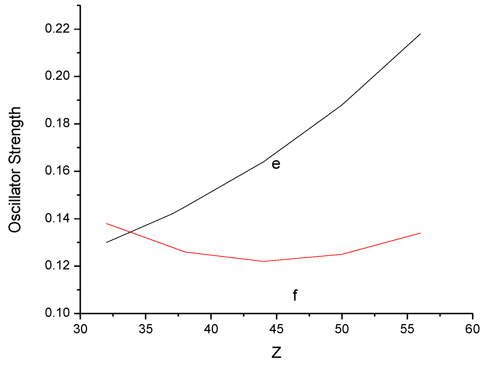
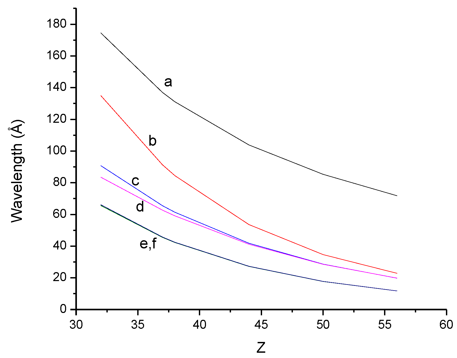
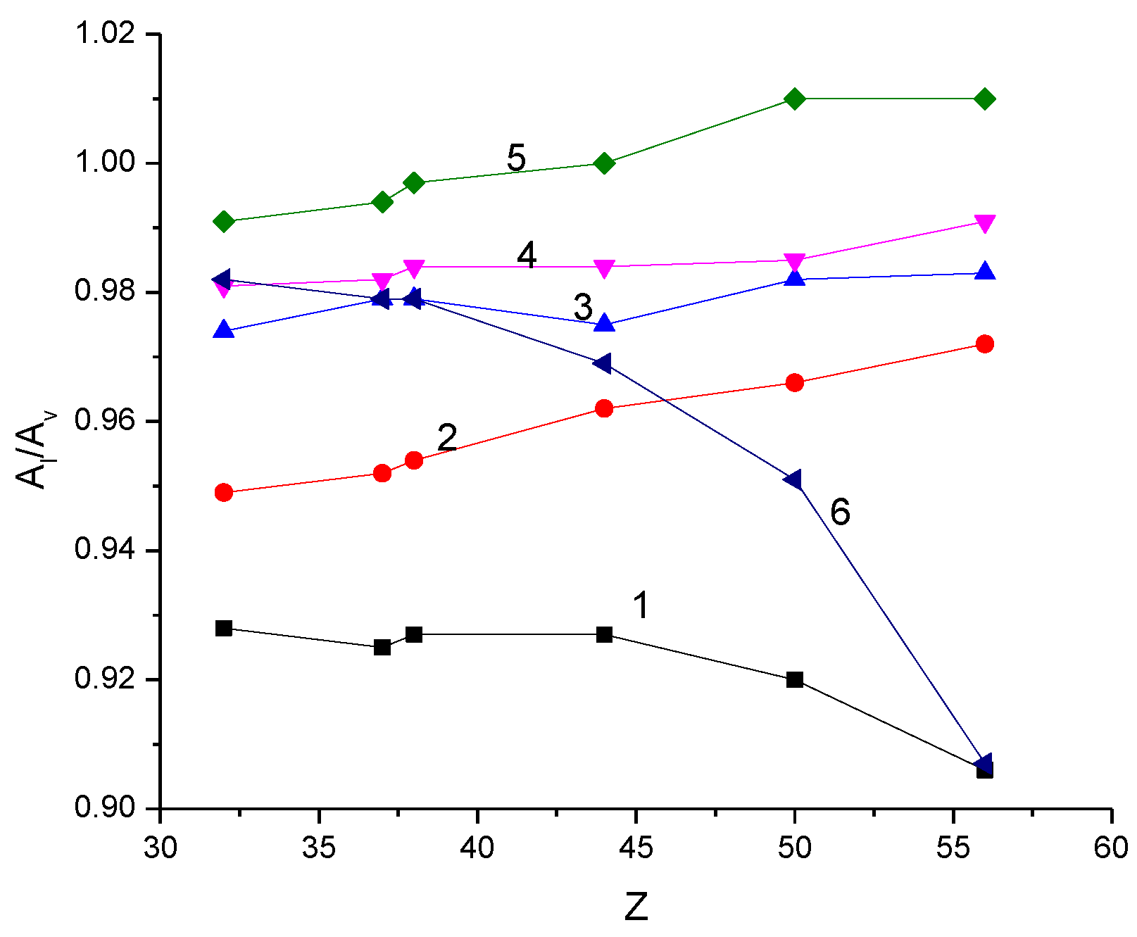
3. Results and Discussion
4. Conclusions
Acknowledgments
Author Contributions
Conflicts of Interest
References
- Landi, E.; Gu, M.F. Atomic data for high-energy configurations in Fe xvii–xxiii. Astrophys. J. 2006, 640, 1171–1179. [Google Scholar] [CrossRef]
- Vilkas, M.J.; Ishikawa, Y.; Träbert, E. Relativistic Many-Body Perturbation Calculations of Boron-Like Silicon, Si X. Phys. Scr. 2005, 72, 181–199. [Google Scholar] [CrossRef]
- Jonauskas, V.; Bogdanovich, P.; Keenan, F.P.; Kisielius, R.; Roord, M.E.; Heeter, R.F.; Rose, S.J.; Ferland, G.J.; Norrington, P.H. Energy levels and transition probabilities for boron-like Fe XXII. Astron. Astrophys. 2006, 455, 1157–1160. [Google Scholar] [CrossRef]
- Wouters, A.; Schwob, J.L.; Suckewer, S.; Seely, J.F.; Feldman, U.; Dave, J.H. Spectra in the 60345-Å wavelength region of the elements Fe, Ni, Zn, Ge, Se, and Mo injected into the Princeton Large Torus tokamak. J. Opt. Soc. Am. B 1988, 5, 1520–1527. [Google Scholar] [CrossRef]
- Myrnäs, R.; Jupen, C.; Miecnik, G.; Martinson, I.; Denne-Hinnov, B. Transitions in boronlike Ni XXIV, Ge XXVIII, Kr XXXII and Mo XXXVIII and fluorinelike Zr XXXII and Mo XXXIV, observed in the JET tokamak. Phys. Scr. 1994, 49, 429. [Google Scholar] [CrossRef]
- Galavís, M.; Mendoza, C.; Zeippen, C. Atomic data from the Iron Project XXIX: Radiative rates for transitions within the n = 2 complex in ions of the boron isoelectronic sequence. Astron. Astrophys. Suppl. Ser. 1998, 131, 499–522. [Google Scholar] [CrossRef]
- Doschek, G.A.; Meekins, J.F.; Cowan, R.D. Spectra of solar flares from 8.5 Å to 16 Å. Sol. Phys. 1973, 29, 125–141. [Google Scholar] [CrossRef]
- Mason, H.E.; Storey, P.J. Atomic data for Fe XII. Mon. Not. R. Astron. Soc. 1980, 191, 631–639. [Google Scholar] [CrossRef]
- Machtoub, G.; López-Urrutia, J.R.C.; Zhang, X.; Tawara, H. Electron–ion interactions for trapped highly charged Ge ions. Can. J. Phys. 2006, 84, 67–81. [Google Scholar] [CrossRef]
- Cheng, K.T.; Kim, Y.K.; Desclaux, J.P. Electric dipole, quadrupole, and magnetic dipole transition probabilities of ions isoelectronic to the first-row atoms, Li through F. At. Data Nucl. Data Tables 1979, 24, 111–189. [Google Scholar] [CrossRef]
- Safronova, U.I.; Johnson, W.R.; Safronova, M.S. Relativistic many-body calculations of energies of n = 3 states for the boron isoelectronic sequence, Z = 6–30. At. Data Nucl. Data Tables 1998, 69, 183–215. [Google Scholar] [CrossRef]
- Zhang, H.L.; Sampson, D.H. Relativistic Distorted-Wave Collision Strengths and Oscillator Strengths for the 105 Δn = 0 Transitions with n = 2 in the 85 B-Like Ions with 8 ≤ Z ≤ 92. At. Data Nucl. Data Tables 1994, 56, 41–104. [Google Scholar] [CrossRef]
- Vilkas, M.J.; Ishikawa, Y.; Koc, K. Second-order multiconfigurational Dirac–Fock calculations on boronlike ions (pages 813–823). Int. J. Quant. Chem. 1998, 70, 813–823. [Google Scholar] [CrossRef]
- Shirai, T.; Reader, J.; Kramida, A.E.; Sugar, J. Spectral Data for Gallium: Ga I through Ga XXXI. J. Phys. Chem. Ref. Data 2007, 36, 509–615. [Google Scholar] [CrossRef]
- Nahar, S.N. Allowed and forbidden transition parameters for Fe XXII. At. Data Nucl. Data Tables 2010, 96, 26–51. [Google Scholar] [CrossRef]
- Murakami, I.; Safronova, U.I.; Vasilyev, A.A.; Kato, T. Excitation energies, radiative and autoionization rates, dielectronic satellite lines, and dielectronic recombination rates to excited states for B-like oxygen. At. Data Nucl. Data Tables 2005, 90, 1–74. [Google Scholar] [CrossRef]
- Bhatia, A.K.; Feldman, U.; Seely, J.F. Atomic data and spectral line intensities for the boron isoelectronic sequence (Ar XIV through Kr XXXII). At. Data Nucl. Data Tables 1986, 35, 319–343. [Google Scholar] [CrossRef]
- Tachiev, G.; Fischer, C.F. Breit–Pauli energy levels, lifetimes, and transition probabilities for the beryllium-like to neon-like sequences. At. Data Nucl. Data Tables 2004, 87, 1–184. [Google Scholar]
- Tachiev, G.; Fischer, C.F. Breit-Pauli energy levels, lifetimes and transition data: Boron-like spectra. J. Phys. B At. Mol. Opt. Phys. 2000, 33, 2419–2435. [Google Scholar] [CrossRef]
- Fischer, C.F.; Tachiev, G. MCHF/MCDHF Collection, Version 2, Ref. No. 3, 40, National Institute of Standards and Technology. 2011. Available online: http://physics.nist.gov/mchf (accessed on 8 April 2016). [Google Scholar]
- Koc, K. Ab initio calculation of 1s22l3l'4l'' energy levels and E1 transition probabilities for O3+. J. Phys. B At. Mol. Opt. Phys. 2004, 37, 3821–3835. [Google Scholar] [CrossRef]
- Koc, K. Relativistic MR RCI Calculation of Energy Levels and Transition Probabilities of Boron Isoelectronic Sequence. Phys. Scr. 2003, 67, 491–499. [Google Scholar] [CrossRef]
- Koc, K. QED effects in transition energies of low lying levels for highly ionized boron like ions. Nucl. Instr. Meth. Phys. Res. B 2005, 235, 46–50. [Google Scholar] [CrossRef]
- Corrégé, G.; Hibbert, A. Transitions in C II, N III, and O IV. At. Data Nucl. Data Tables 2004, 86, 19–34. [Google Scholar] [CrossRef]
- Jönsson, P.; Li, J.; Gaigalas, G.; Dong, C. Hyperfine structures, isotope shifts, and transition rates of C II, N III, and O IV from relativistic configuration interaction calculations. At. Data Nucl. Data Tables 2010, 96, 271–298. [Google Scholar] [CrossRef]
- Li, J.; Jönsson, P.; Dong, C.; Gaigalas, G. Two-electron–one-photon M1 and E2 transitions between the states of the 2p3 and 2s22p odd configurations for B-like ions with 18 ≤ Z ≤ 92. J. Phys. B At. Mol. Opt. Phys. 2010, 43, 035005. [Google Scholar] [CrossRef]
- Hao, L.; Jiang, G. Energy levels, transition rates, and line strengths of B-like ions. Phys. Rev. A 2011, 83, 012511. [Google Scholar] [CrossRef]
- Rynkun, P.; Jönsson, P.; Gaigalas, G.; Fischer, C.F. Energies and E1, M1, E2, M2 transition rates for states of the 2s22p, 2s2p2, and 2p3 configurations in boron-like ions between N III and Zn XXVI. At. Data Nucl. Data Tables 2012, 98, 481–556. [Google Scholar] [CrossRef]
- Marques, J.P.; Indelicato, P.; Parente, F. Relativistic multiconfiguration calculations of the 2s22p 2P3/2 level lifetime along the boron isoelectronic sequence. Eur. Phys. J. D 2012, 66, 32. [Google Scholar] [CrossRef]
- Zhang, C.M.; Chen, C.; Sun, Y.; Gou, B.C.; Shao, B. Energy, fine structure, hyperfine structure, and radiative transition rates of the high-lying multi-excited states for B-like neon Eur. Phys. J. D 2015, 69, 105. [Google Scholar]
- Chen, C. Energies, expectation values, fine structures and hyperfine structures of the ground state and excited states for boron. Eur. Phys. J. D 2015, 69, 128. [Google Scholar] [CrossRef]
- Reader, J.; Gillaspy, J.D.; Osin, D.; Ralchenko, Y. Extreme ultraviolet spectra and analysis of Δn = 0 transitions in highly charged barium. J. Phys. B At. Mol. Opt. Phys. 2014, 47, 145003. [Google Scholar] [CrossRef]
- Jönsson, P.; He, X.; Fischer, C.F.; Grant, I.P. The grasp2K relativistic atomic structure package. Comput. Phys. Commun. 2007, 177, 597–622. [Google Scholar] [CrossRef]
- Grant, I.P. Relativistic Quantum Theory of Atoms and Molecules; Springer: New York, NY, USA, 2007. [Google Scholar]
- McKenzie, B.J.; Grant, I.P.; Norrington, P.H. A program to calculate transverse Breit and QED corrections to energy levels in a multiconfiguration Dirac-Fock environment. Comput. Phys. Commun. 1980, 21, 233–246. [Google Scholar] [CrossRef]
- Gaigalas, G.; Rudzikas, Z.; Fischer, C.F. An efficient approach for spin-angular integrations in atomic structure calculations. J. Phys. B At. Mol. Opt. Phys. 1997, 30, 3747–3771. [Google Scholar] [CrossRef]
- Grant, I.P. Gauge invariance and relativistic radiative transitions. J. Phys. B. At. Mol. Opt. Phys. 1974, 7, 1458–1475. [Google Scholar] [CrossRef]
- Dyall, K.G.; Grant, I.P.; Johnson, C.T.; Parpia, F.A.; Plummer, E.P. GRASP: A general-purpose relativistic atomic structure program. Comput. Phys. Commun. 1989, 55, 425–456. [Google Scholar] [CrossRef]
- Olsen, J.; Roos, B.O.; Jorgensen, P.; Jensen, H.J.A. Determinant based configuration interaction algorithms for complete and restricted configuration interaction spaces. J. Chem. Phys. 1988, 89, 2185–2192. [Google Scholar] [CrossRef]
- Sturesson, L.; Jönsson, P.; Fischer, C.F. JJGEN: A flexible program for generating lists of jj-coupled configuration state functions Comput. Phys. Commun. 2007, 177, 539–550. [Google Scholar] [CrossRef]
- Oslen, J.; Godefroid, M.R.; Jönsson, P.A.; Malmquist, P.A.; Froese, F.C. Transition probability calculations for atoms using nonorthogonal orbitals. Phys. Rev. E 1995, 52, 4499–4508. [Google Scholar]
- Norrington, P.H.; Kingston, A.E.; Boone, A.W. Energy levels and transition probabilities for Fe XXV ions. J. Phys. B At. Mol. Opt. Phys. 2000, 33, 1767–1788. [Google Scholar] [CrossRef]
- Kramida, A.; Ralchenko, Y.; Reader, J.; NIST ASD Team. NIST Atomic Spectra Database (ver. 5.3); National Institute of Standards and Technology: Gaitherburg, MD, USA, 2015; Available online: http://physics.nist.gov/asd (accessed on 23 November 2015).
- Kramida, A.; Ralchenko, Y.; Reader, J.; NIST ASD Team. NIST Atomic Spectra Database (ver. 5.2); National Institute of Standards and Technology: Gaitherburg, MD, USA, 2014; Available online: http://physics.nist.gov/asd (accessed on 26 August 2015).
- Farrag, A.; Luc-Koenig, E.; Sinzelle, J. Systematic trends of the relativistic f values for electric dipole transitions within the ground complex of B-like ions. J. Phys. B At. Mol. Opt. Phys. 1980, 13, 3939–3955. [Google Scholar] [CrossRef]


| Ge | ||||||||||
| Configuration | VV | CV | ||||||||
| n = 4 | n = 5 | n = 6 | n = 7 | n = 4 | n = 5 | n = 6 | n = 7 | Ref. [17] | Δ% | |
| 2s2 2p 2P° 1/2 | 0.00 | 0.00 | 0.00 | 0.00 | 0.00 | 0.00 | 0.00 | 0.00 | 0.00 | 0.00 |
| 2s2 2p 2P° 3/2 | 294,359.19 | 294,335.58 | 294,358.61 | 294,371.64 | 294,445.85 | 294,544.84 | 294,700.43 | 294,824.39 | 294,539 | 0.09 |
| 294,658a | 0.06 | |||||||||
| 294,668b | 0.05 | |||||||||
| 294,550c | 0.09 | |||||||||
| 294,614d | 0.07 | |||||||||
| 2s2p2 4P1/2 | 572,810.09 | 573,172.37 | 573,274.34 | 573,321.06 | 572,252.78 | 572,596.33 | 572,794.37 | 572,943.86 | 574,559 | 0.28 |
| 573,139a | 0.03 | |||||||||
| 572,858b | 0.01 | |||||||||
| 2s2p2 4P3/2 | 740,529.66 | 740,925.26 | 741,020.59 | 741,066.48 | 740,080.93 | 740,426.04 | 740,591.13 | 740,721.62 | 742,598 | 0.25 |
| 2s2p2 4P5/2 | 846,036.05 | 846,212.79 | 846,272.93 | 846,303.89 | 845,542.28 | 845,510.69 | 845,513.03 | 845,531.07 | 847,406 | 0.22 |
| 2s2p2 2D3/2 | 1,103,153.70 | 1,102,793.77 | 1,102,766.60 | 1,102,760.55 | 1,102,276.49 | 1,101,807.99 | 1,101,836.13 | 1,101,909.39 | 1,102,111 | 0.02 |
| 2s2p2 2P1/2 | 1,199,600.45 | 1,199,379.88 | 1,199,412.07 | 1,199,425.53 | 1197969.03 | 1197600.77 | 1,197,678.13 | 1,197,770.15 | 1,197,323 | 0.04 |
| 2s2p2 2D5/2 | 1,211,205.85 | 1,210,750.86 | 1,210,686.99 | 1,210,664.84 | 1,210,505.67 | 1,209,856.50 | 1,209,748.39 | 1,209,723.04 | 1,211,608 | 0.15 |
| 2s2p2 2S1/2 | 1,513,917.87 | 1,513,582.64 | 1,513,577.79 | 1,513,573.67 | 1,512,905.95 | 1,512,529.92 | 1,512,614.73 | 1,512,712.55 | 1,505,579 | 0.47 |
| 2s2p2 2P3/2 | 1,527,073.63 | 1,526,714.16 | 1,526,697.23 | 1,526,695.12 | 1525292.77 | 1524737.12 | 1,524,740.20 | 1,524,799.94 | 1,523,491 | 0.08 |
| Rb | ||||||||||
| Configuration | VV | CV | ||||||||
| n = 4 | n = 5 | n = 6 | n = 7 | n = 4 | n = 5 | n = 6 | n = 7 | Other | Δ% | |
| 2s22p 2P° 1/2 | 0.00 | 0.00 | 0.00 | 0.00 | 0.00 | 0.00 | 0.00 | 0.00 | 0.00 | 0.00 |
| 2s22p 2P° 3/2 | 554,879.16 | 554,870.27 | 554,891.60 | 554,907.79 | 554,994.57 | 555,105.27 | 555,259.44 | 555,379.85 | 554,700c | 0.12 |
| 555,329a | 0.01 | |||||||||
| 555,338b | 0.01 | |||||||||
| 2s2p2 4P1/2 | 730,395.31 | 730,657.17 | 730,740.17 | 730,781.53 | 729,723.78 | 729,940.10 | 730,109.73 | 730,241.58 | 726,900c | 0.46 |
| 730,429a | 0.02 | |||||||||
| 730,041b | 0.03 | |||||||||
| 2s2p2 4P3/2 | 1,095,432.10 | 1,095,811.16 | 1,095,900.17 | 1,095,946.77 | 1,094,951.96 | 1,095,471.35 | 1,095,401.41 | 1,095,517.75 | 1,089,900c | 0.51 |
| 2s2p2 4P5/2 | 1,245,199.88 | 1,245,245.18 | 1,245,275.42 | 1,245,296.70 | 1,244,612.54 | 1,244,431.32 | 1,244,402.22 | 1,244,404.33 | 1,242,100c | 0.18 |
| 2s2p2 2D3/2 | 1,527,957.94 | 1,527,589.89 | 1,527,553.99 | 1,527,548.25 | 1,527,778.22 | 1,526,581.58 | 1,526,417.03 | 1,526,473.27 | 1,532,900c | 0.42 |
| 2s2p2 2P1/2 | 1,597,246.42 | 1,597,079.83 | 1,597,124.78 | 1,597,147.92 | 1,595,466.01 | 1,595,131.27 | 1,595,213.20 | 1,595,303.30 | 1,604,400c | 0.57 |
| 2s2p2 2D5/2 | 1,814,677.32 | 1,814,403.75 | 1,814,366.82 | 1,814,358.66 | 1,814,002.12 | 1,813,535.33 | 1,813,459.03 | 1,813,444.10 | 1,814,700c | 0.07 |
| 2s2p2 2S1/2 | 2,187,867.67 | 2,187,546.02 | 2,187,542.46 | 2,187,542.52 | 2,186,881.54 | 2,186,524.70 | 2,186,614.52 | 2,186,711.39 | 2,191,200c | 0.20 |
| 2s2p2 2P3/2 | 2,199,518.57 | 2,199,195.73 | 2,199,184.27 | 2,199,188.43 | 2,198,582.20 | 2,197,311.71 | 2,197,213.85 | 2,197,269.66 | 2,207,900c | 0.48 |
| Sr | ||||||||||
| Configuration | VV | CV | ||||||||
| n = 4 | n = 5 | n = 6 | n = 7 | n = 4 | n = 5 | n = 6 | n = 7 | Other | Δ% | |
| 2s22p 2P° 1/2 | 0.00 | 0.00 | 0.00 | 0.00 | 0.00 | 0.00 | 0.00 | 0.00 | 0.00 | 0.00 |
| 2s22p 2P° 3/2 | 623,284.03 | 623,275.74 | 623,301.64 | 623,316.67 | 623,405.36 | 623,519.82 | 623,675.76 | 623,379.36 | 623,100c | 0.04 |
| 623,739a | 0.06 | |||||||||
| 623,747b | 0.06 | |||||||||
| 2s2p2 4P1/2 | 763,024.73 | 763,262.18 | 763,345.64 | 763,384.59 | 762,324.87 | 762,514.86 | 762,679.97 | 762,807.35 | 759,800c | 0.39 |
| 762,976a | 0.02 | |||||||||
| 762,565b | 0.03 | |||||||||
| 2s2p2 4P3/2 | 1,183,539.38 | 1,183,909.04 | 1,184,000.99 | 1,184,046.38 | 1,183,036.48 | 1,183,318.82 | 1,183,448.77 | 1,183,551.33 | 1,178,000c | 0.47 |
| 2s2p2 4P5/2 | 1,341,468.23 | 1,341,487.09 | 1,341,515.58 | 1,341,534.53 | 1,340,860.77 | 1,340,652.95 | 1,340,618.81 | 1,340,617.83 | 1,338,600c | 0.15 |
| 2s2p2 2D3/2 | 1,629,937.45 | 1,629,540.42 | 1,629,503.96 | 1,629,495.58 | 1,628,859.19 | 1,628,304.40 | 1,628,288.42 | 1,628,331.20 | 1,634,900c | 0.40 |
| 2s2p2 2P1/2 | 1,693,721.64 | 1,693,562.92 | 1,693,614.61 | 1,693,638.49 | 1,691,914.66 | 1,691,588.56 | 1,691,673.26 | 1,691,762.37 | 1,700,800c | 0.53 |
| 2s2p2 2D5/2 | 1,969,084.81 | 1,968,840.72 | 1,968,812.81 | 1,968,807.12 | 1,968,414.67 | 1,967,981.54 | 1,967,912.63 | 1,967,900.11 | 1,968,800c | 0.04 |
| 2s2p2 2S1/2 | 2,355,943.75 | 2,355,623.32 | 2,355,624.88 | 2,355,624.75 | 2,354,959.94 | 2,354,609.24 | 2,354,702.02 | 2,354,798.15 | 2,359,100c | 0.18 |
| 2s2p2 2P3/2 | 2,367,421.82 | 2,367,072.08 | 2,367,061.00 | 2,367,063.13 | 2,365,622.03 | 2,365,064.97 | 2,365,055.70 | 2,365,100.13 | 2,375,500c | 0.44 |
| Ru | ||||||||||
| Configuration | VV | CV | ||||||||
| n = 4 | n = 5 | n = 6 | n = 7 | n = 4 | n = 5 | n = 6 | n = 7 | Ref. [23] | Δ% | |
| 2s22p 2P° 1/2 | 0.00 | 0.00 | 0.00 | 0.00 | 0.00 | 0.00 | 0.00 | 0.00 | 0.00 | |
| 2s2p2 4P1/2 | 963,735.96 | 963,847.87 | 963,910.53 | 963,929.75 | 962,833.63 | 962,867.47 | 962,993.35 | 963,105.03 | 963,285a | 0.02 |
| 962,734b | 0.04 | |||||||||
| 2s22p 2P° 3/2 | 1,180,758.61 | 1,180,767.78 | 1,180,797.79 | 1,180,804.10 | 1,180,916.59 | 1,181,063.55 | 1,181,219.58 | 1,181,344.53 | 1,181,453a | 0.01 |
| 1,181,450b | 0.01 | |||||||||
| 2s2p2 4P3/2 | 1,865,365.70 | 1,865,718.29 | 1,865,804.50 | 1,865,836.54 | 1,864,874.29 | 1,865,056.33 | 1,865,163.52 | 1,865,257.38 | ||
| 2s2p2 4P5/2 | 2,066,640.94 | 2,066,553.94 | 2,066,559.15 | 2,066,556.66 | 2,065,913.40 | 2,065,586.26 | 2,065,510.67 | 2,065,498.15 | ||
| 2s2p2 2D3/2 | 2,393,724.80 | 2,393,327.09 | 2,393,285.00 | 2,393,262.22 | 2,392,484.98 | 2,391,858.98 | 2,391,815.83 | 2,391,847.82 | ||
| 2s2p2 2P1/2 | 2,428,031.86 | 2,427,931.61 | 2,427,998.54 | 2,428,019.48 | 2,426,075.45 | 2,425,798.57 | 2,425,886.93 | 2,425,980.87 | ||
| 2s2p2 2D5/2 | 3,199,253.57 | 3,199,167.00 | 3,199,170.59 | 3,199,166.72 | 3,198,607.59 | 3,198,345.46 | 3,198,301.12 | 3,198,306.13 | ||
| 2s2p2 2S1/2 | 3,665,385.67 | 3,665,095.71 | 3,665,106.49 | 3,665,100.75 | 3,664,395.96 | 3,465,296.95 | 3,465,029.12 | 3,464,957.16 | ||
| 2s2p2 2P3/2 | 3,676,012.00 | 3,675,708.30 | 3,675,706.90 | 3,675,701.93 | 3,674,204.06 | 3,664,086.23 | 3,664,186.22 | 3,664,289.99 | ||
| Sn | ||||||||||
| Configuration | VV | CV | ||||||||
| n = 4 | n = 5 | n = 6 | n = 7 | n = 4 | n = 5 | n = 6 | n = 7 | Ref. [23] | Δ% | |
| 2s22p 2P° 1/2 | 0.00 | 0.00 | 0.00 | 0.00 | 0.00 | 0.00 | 0.00 | 0.00 | 0.00 | |
| 2s2p2 4P1/2 | 1,172,932.39 | 1,172,931.39 | 1,172,977.25 | 1,173,002.49 | 1,171,793.52 | 1,171,681.51 | 1,171,782.28 | 1,171,874.84 | 1,172,053a | 0.01 |
| 1,171,358b | 0.04 | |||||||||
| 2s22p 2P° 3/2 | 2,063,472.21 | 2,063,518.86 | 2,063,547.86 | 2,063,572.30 | 2,063,683.87 | 2,063,868.26 | 2,064,045.18 | 2,064,175.01 | 2,064,478a | 0.01 |
| 2,064,448b | 0.01 | |||||||||
| 2s2p2 4P3/2 | 2,884,412.96 | 2,884,756.24 | 2,884,839.77 | 2,884,884.61 | 2,883,794.52 | 2,884,027.38 | 2,884,133.52 | 2,884,220.49 | ||
| 2s2p2 2D5/2 | 3,121,078.42 | 3,120,936.00 | 3,120,931.84 | 3,120,935.40 | 3,120,228.30 | 3,119,821.85 | 3,119,731.04 | 3,119,706.80 | ||
| 2s2p2 2D3/2 | 3,493,429.54 | 3,493,073.93 | 3,493,038.56 | 3,493,033.78 | 3,491,945.09 | 3,491,391.15 | 3,491,352.02 | 3,491,378.27 | ||
| 2s2p2 2P1/2 | 3,505,894.95 | 3,505,837.96 | 3,505,919.22 | 3,505,960.42 | 3,503,775.07 | 3,503,534.71 | 3,503,638.30 | 3,503,732.41 | ||
| 2s2p2 4P5/2 | 5,096,696.59 | 5,096,720.50 | 5,096,752.03 | 5,096,771.52 | 5,096,062.17 | 4,761,571.79 | 4,761,262.07 | 4,761,169.15 | ||
| 2s2p2 2S1/2 | 5,640,312.35 | 5,640,057.95 | 5,640,081.85 | 5,640,096.00 | 5,639,304.58 | 5,095,918.02 | 5,095,910.46 | 5,095,927.34 | ||
| 2s2p2 2P3/2 | 5,650,330.14 | 5,650,123.49 | 5,650,145.57 | 5,650,165.52 | 5,648,454.69 | 5,639,044.37 | 5,639,168.23 | 5,639,277.45 | ||
| Ba | ||||||||||
| Configuration | VV | CV | ||||||||
| n = 4 | n = 5 | n = 6 | n = 7 | n = 4 | n = 5 | n = 6 | n = 7 | Ref. [23] | Δ% | |
| 2s22p 2P° 1/2 | 0.00 | 0.00 | 0.00 | 0.00 | 0.00 | 0.00 | 0.00 | 0.00 | ||
| 2s2p2 4P1/2 | 1,394,480.97 | 1,394,373.83 | 1,394,398.45 | 1,394,422.04 | 1,393,070.22 | 1,392,820.60 | 1,392,896.06 | 1,392,944.14 | ||
| 1,393,276a | 0.02 | |||||||||
| 1,392,459b | 0.03 | |||||||||
| 2s22p 2P° 3/2 | 3,393,333.19 | 3,393,412.40 | 3,393,454.03 | 3,393,489.63 | 3,393,607.70 | 3,393,850.70 | 3,394,049.82 | 3,394,191.00 | ||
| 3,394,759a | 0.02 | |||||||||
| 3,394,676b | 0.01 | |||||||||
| 2s2p2 4P3/2 | 4,365,092.43 | 4,365,428.44 | 4,365,506.06 | 4,365,555.28 | 4,364,405.03 | 4,364,626.73 | 4,364,728.87 | 4,364,816.11 | ||
| 2s2p2 2D5/2 | 4,631,483.73 | 4,631,314.92 | 4,631,300.47 | 4,631,309.82 | 4,630,674.88 | 4,630,045.47 | 4,629,940.55 | 4,629,909.23 | ||
| 2s2p2 2P1/2 | 5,052,120.83 | 5,052,094.24 | 5,052,183.32 | 5,052,236.95 | 5,049,800.11 | 5,049,589.51 | 5,049,709.12 | 5,049,720.16 | ||
| 2s2p2 2D3/2 | 5,054,465.27 | 5,054,148.70 | 5,054,121.67 | 5,054,125.23 | 5,052,767.66 | 5,052,245.40 | 5,052,210.60 | 5,052,239.37 | ||
| 2s2p2 4P5/2 | 7,905,439.73 | 7,905,551.78 | 7,905,601.74 | 7,905,639.21 | 7,904,940.53 | 6,535,783.59 | 6,535,433.14 | 6,535,318.45 | ||
| 2s2p2 2S1/2 | 8,528,078.13 | 8,527,865.22 | 8,527,899.71 | 8,527,927.19 | 8,527,043.94 | 7,904,769.39 | 7,904,793.46 | 7,904,826.22 | ||
| 2s2p2 2P3/2 | 8,537,396.20 | 8,537,283.19 | 8,537,328.52 | 8,537,364.66 | 8,535,451.45 | 8,526,851.59 | 8,527,006.46 | 8,527,195.97 | ||
| Ge | ||
| Level | Mix | Contribution |
| 2s22p 2P°1/2 | 0.99 (1) + 0.12 (2p3 2P°1/2) | 0.98 (1) + 0.01 (2p3 2P°1/2) |
| 2s22p 2P°3/2 | 0.99 (2) + 0.14 (2p3 2P°3/2) | 0.98 (2) + 0.02 (2p3 2P°3/2) |
| 2s2p2 4P1/2 | 0.94 (3) + 0.30 (9) + 0.13 (7) | 0.89 (2s2p2 4P1/2) + 0.09 (9) + 0.02 (7) |
| 2s2p2 4P3/2 | –0.99 (4) + 0.11 (6)+ 0.08 (10) | –0.99 (4) + 0.11 (6) + 0.08 (10) |
| 2s2p2 4P5/2 | 0.90 (5) – 0.43 (8) | 0.81 (5) + 0.19 (8) |
| 2s2p2 2D3/2 | 0.93 (6) + 0.34 (10) + 0.08 (4) | 0.87 (6) + 0.12 (10) + 0.01 (4) |
| 2s2p2 2P1/2 | 0.84 (7) + 0.47 (9) + 0.27 (3) | 0.70 (7) + 0.22 (9) + 0.07 (3) |
| 2s2p2 2D5/2 | 0.90(8) + 0.43 (5) | 0.81 (8) + 0.19 (5) |
| 2s2p2 2S1/2 | 0.82 (9) – 0.52 (7) – 0.19(3) | 0.69 (9) + 0.27 (7) + 0.04 (3) |
| 2s2p2 2P3/2 | 0.93 (10) – 0.33 (6) – 0.11 (4) | 0.87 (2s2p2 2P3/2) + 0.11 (6) + 0.01 (4) |
| Rb | ||
| Level | Mix | Contribution |
| 2s22p 2P°1/2 | 0.99 (1) + 0.11 (2p3 2P°1/2) | 0.99 (1) + 0.01(2p3 2P°1/2) |
| 2s22p 2P°3/2 | 0.99 (2) + 0.14 (2p3 2P°3/2) | 0.98 (2) + 0.02 (2p3 2P°3/2) |
| 2s2p2 4P1/2 | 0.90 (3) + 0.39 (9) + 0.20 (7) | 0.80 (3) + 0.15 (9) + 0.04 (7) |
| 2s2p2 4P3/2 | –0.98 (4) + 0.15 (6) – 0.10 (10) | 0.97 (4) + 0.02 (6) + 0.01 (10) |
| 2s2p2 4P5/2 | 0.82 (5) – 0.57 (8) | 0.67 (5) + 0.32 (8) |
| 2s2p2 2D3/2 | 0.90 (6) + 0.43 (10) +0.09 (4) | 0.80 (6) + 0.19 (10) +0.01 (4) |
| 2s2p2 2P1/2 | 0.85 (7) +0.37 (9) – 0.36 (3) | 0.73 (7) + 0.14 (9) + 0.13 (3) |
| 2s2p2 2D5/2 | 0.82 (8) + 0.57(5) | 0.67(8) + 0.32 (5) |
| 2s2p2 2S1/2 | 0.84 (9) – 0.47 (7) – 0.25 (3) | 0.77 (9) + 0.22 (7) + 0.07 (3) |
| 2s2p2 2P3/2 | 0.89 (10) – 0.41 (6) – 0.16 (4) | 0.80 (10) + 0.17 (6) + 0.02 (4) |
| Sr | ||
| Level | Mix | Contribution |
| 2s22p 2P°1/2 | 0.99 (1) + 0.10 (2p3 2P°1/2) | 0.99 (1) + 0.01 (2p3 2P°1/2) |
| 2s22p 2P°3/2 | 0.99 (2) + 0.13 (2p3 2P°3/2) | 0.98(2) + 0.02 (2p3 2P°3/2) |
| 2s2p2 4P1/2 | 0.89 (3) + 0.41 (9) + 0.22 (7) | 0.78 (3) + 0.16 (9) + 0.05 (7) |
| 2s2p2 4P3/2 | –0.98 (4) + 0.16 (6) – 0.11 (10) | 0.96 (4) + 0.02 (6) – 0.01 (10) |
| 2s2p2 4P5/2 | 0.80 (5) – 0.59 (8) | 0.65(5) + 0.35 (8) |
| 2s2p2 2D3/2 | 0.89 (6) – 0.43 (10) – 0.16 (4) | 0.79 (6) + 0.20 (10) +0.01 (4) |
| 2s2p2 2P1/2 | 0.86 (7) – 0.37 (3) + 0.35 (9) | 0.73 (7) – 0.14 (3) + 0.12 (9) |
| 2s2p2 2D5/2 | 0.80 (8) + 0.59 (5) | 0.65 (8) + 0.35(5) |
| 2s2p2 2S1/2 | 0.84 (9) – 0.46 (7) – 0.27 (3) | 0.71 (9) + 0.21 (7) + 0.07 (3) |
| 2s2p2 2P3/2 | 0.89 (10) – 0.43 (6) – 0.16 (4) | 0.79 (10) + 0.18 (6) + 0.03 (4) |
| Ru | ||
| Level | Mix | Contribution |
| 2s22p 2P°1/2 | 0.99 (1) + 0.08 (2p3 2P°1/2) | 0.99 (1) + 0.01 (2p3 2P°1/2) |
| 2s22p 2P°3/2 | 0.99 (2) + 0.12 (2p3 2P°3/2) | 0.98(2) + 0.01 (2p3 2P°3/2) |
| 2s2p2 4P1/2 | 0.83 (3) + 0.47 (9) + 0.30 (7) | 0.69 (3) + 0.22 (9) + 0.09 (7) |
| 2s2p2 4P3/2 | –0.97 (4) + 0.19 (6) – 0.13 (10) | 0.95 (4) + 0.04 (6) + 0.02 (10) |
| 2s2p2 4P5/2 | 0.73(5) – 0.68 (8) | 0.53 (5) + 0.47 (8) |
| 2s2p2 2D3/2 | 0.85 (6) – 0.51 (10) – 0.10 (4) | 0.73 (6) + 0.26 (10) +0.01 (4) |
| 2s2p2 2P1/2 | 0.85 (7) – 0.45 (3) + 0.25 (9) | 0.73 (7) + 0.20 (3) +0.06 (9) |
| 2s2p2 2D5/2 | 0.73(8) + 0.68 (5) | 0.53 (8) + 0.47 (5) |
| 2s2p2 2S1/2 | 0.84 (9) – 0.42 (7) – 0.33 (3) | 0.71 (9) + 0.18 (7) + 0.11 (3) |
| 2s2p2 2P3/2 | 0.85 (10) – 0.48 (6) – 0.21 (4) | 0.72 (10) + 0.24 (6) + 0.04 (4) |
| Sn | ||
| Level | Mix | Contribution |
| 2s22p 2P°1/2 | 0.99 (1) + 0.07 (2p3 2P°1/2) | 0.99 (1) + 0.00 (2p3 2P°1/2) |
| 2s22p 2P°3/2 | 0.99 (2) + 0.11 (2p3 2P°3/2) | 0.98 (2) + 0.01 (2p3 2P°3/2) |
| 2s2p2 4P1/2 | 0.78 (3) + 0.51 (9) + 0.35 (7) | 0.61 (3) + 0.26 (9) + 0.12 (7) |
| 2s2p2 4P3/2 | –0.96 (4) + 0.22 (6) – 0.14 (10) | 0.93 (4) + 0.05 (6) + 0.02 (10) |
| 2s2p2 2D5/2 | –0.73 (5) + 0.68 (8) | 0.54 (5) + 0.46 (8) |
| 2s2p2 2D3/2 | 0.83 (6) − 0.55 (10) + 0.10 (4) | 0.68 (6) + 0.31 (10) + 0.01 (4) |
| 2s2p2 2P1/2 | 0.85 (7) – 0.50 (3) + 0.18 (9) | 0.72 (7) + 0.25 (3) + 0.03 (9) |
| 2s2p2 4P5/2 | 0.73 (8) + 0.68 (5) | 0.54 (8) + 0.46 (5) |
| 2s2p2 2S1/2 | 0.84 (9) – 0.40 (7) – 0.37 (3) | 0.70 (9) + 0.16 (7) + 0.14 (3) |
| 2s2p2 2P3/2 | 0.82 (10) – 0.52 (6) – 0.24 (4) | 0.67(10) + 0.27 (6) + 0.06 (4) |
| Ba | ||
| Level | Mix | Contribution |
| 2s22p 2P°1/2 | 0.99 (1) + 0.05 (2p3 2P°1/2) | 0.99 (1) + 0.00(2p3 2P°1/2) |
| 2s22p 2P°3/2 | 0.99 (2) + 0.11 (2p3 2P°3/2) | 0.98 (2) + 0.01 (2p3 2P°3/2) |
| 2s2p2 4P1/2 | 0.73 (3) + 0.53 (9) +0.38 (7) | 0.56 (3) + 0.28 (9) +0.14 (7) |
| 2s2p2 4P3/2 | –0.96 (4) + 0.27 (6) – 0.16 (10) | 0.92 (4) +0.05 (6) + 0.02 (10) |
| 2s2p2 2D5/2 | –0.76(5) + 0.64 (8) | 0.58 (5) + 0.42 (8) |
| 2s2p2 2D3/2 | 0.81 (6) + 0.58 (10) + 0.10 (4) | 0.65 (6) + 0.33 (10) + 0.01 (4) |
| 2s2p2 2P1/2 | 0.84 (7) – 0.52 (3) + 0.13 (9) | 0.71 (7) + 0.27 (3) + 0.02 (9) |
| 2s2p2 4P5/2 | 0.76 (8) + 0.64 (5) | 0.58 (8) + 0.42 (5) |
| 2s2p2 2S1/2 | 0.83 (9) – 0.40 (3) – 0.38 (7) | 0.70 (9) + 0.16 (3) + 0.14 (7) |
| 2s2p2 2P3/2 | 0.80 (10) – 0.54 (6) – 0.26 (4) | 0.64(10) + 0.29 (6) + 0.07 (4) |
| VV | |||||||||
| Active set | λ (in Å) | A | gf | S | ΔE (cm−1) | ||||
| n | B | C | B | C | B | C | Sl/Sv | ||
| 3 | 90.35 | 2.67E+10 | 2.96E+10 | 1.31E−01 | 1.45E−01 | 3.89E−02 | 4.31E−02 | 0.902 | 1106813 |
| 4 | 90.65 | 2.64E+10 | 2.84E+10 | 1.30E−01 | 1.40E−01 | 3.88E−02 | 4.18E−02 | 0.928 | 1103153 |
| 5 | 90.68 | 2.63E+10 | 2.85E+10 | 1.30E−01 | 1.41E−01 | 3.88E−02 | 4.20E−02 | 0.924 | 1102793 |
| 6 | 90.68 | 2.63E+10 | 2.85E+10 | 1.30E−01 | 1.41E−01 | 3.88E−02 | 4.20E−02 | 0.924 | 1102766 |
| 7 | 90.68 | 2.63E+10 | 2.85E+10 | 1.30E−01 | 1.41E−01 | 3.88E−02 | 4.20E−02 | 0.924 | 1102760 |
| 90.73e | 1102111e | ||||||||
| CV | |||||||||
| Active set | λ (in Å) | A | gf | S | ΔE (cm−1) | ||||
| n | B | C | B | C | B | C | Sl/Sv | ||
| 3 | 90.37 | 2.67E+10 | 2.83E+10 | 1.31E−01 | 1.39E−01 | 3.89E−02 | 4.12E−02 | 0.944 | 1106581 |
| 4 | 90.72 | 2.63E+10 | 2.68E+10 | 1.30E−01 | 1.32E−01 | 3.87E−02 | 3.96E−02 | 0.977 | 1102276 |
| 5 | 90.76 | 2.62E+10 | 2.69E+10 | 1.30E−01 | 1.33E−01 | 3.87E−02 | 3.96E−02 | 0.977 | 1101807 |
| 6 | 90.76 | 2.62E+10 | 2.69E+10 | 1.30E−01 | 1.33E−01 | 3.87E−02 | 3.96E−02 | 0.977 | 1101836 |
| 7 | 90.75 | 2.62E+10 | 2.69E+10 | 1.30E−01 | 1.33E−01 | 3.87E−02 | 3.96E−02 | 0.977 | 1101909 |
| 90.73e | 1102111e | ||||||||
| Ge | ||||||||||
| Transition | λ (in Å) | λc (in Å) Ref. [17] | A | gf | S | dT | ||||
| i | j | B | C | B | C | B | C | |||
| 2s2 2p 2P°1/2 | 2s2p2 4P1/2 | 174.54 | 174.05 | 5.04E+08 | 5.43E+08 | 4.60E−03 | 4.96E−03 | 2.64E−03 | 2.85E−03 | 0.0719 |
| 2s2 2p 2P°1/2 | 2s2p2 4P3/2 | 135.00 | 134.66 | 1.49E+07 | 1.57E+07 | 1.63E−04 | 1.72E−04 | 7.24E−05 | 7.65E−05 | 0.0539 |
| 2s2 2p 2P°1/2 | 2s2p2 2D3/2 | 90.75 | 90.735 | 2.62E+10 | 2.69E+10 | 1.30E−01 | 1.33E−01 | 3.87E−02 | 3.96E−02 | 0.0233 |
| 2s2 2p 2P°1/2 | 2s2p2 2P1/2 | 83.49 | 83.520 | 6.62E+10 | 6.75E+10 | 1.38E−01 | 1.41E−01 | 3.80E−02 | 3.87E−02 | 0.0188 |
| 2s2 2p 2P°1/2 | 2s2p2 2P3/2 | 65.58 | 65.639 | 7.51E+09 | 7.58E+09 | 1.94E−02 | 1.95E−02 | 4.18E−03 | 4.22E−03 | 0.0086 |
| 2s2 2p 2P°1/2 | 2s2p2 2S1/2 | 66.11 | 66.420 | 1.07E+09 | 1.09E+09 | 1.40E−03 | 1.43E−03 | 3.06E−04 | 3.12E−04 | 0.0199 |
| 2s2 2p 2P°3/2 | 2s2p2 4P1/2 | 359.56 | 357.12 | 1.57E+07 | 1.73E+07 | 6.08E−04 | 6.73E−04 | 7.20E−04 | 7.96E−04 | 0.0953 |
| 2s2 2p 2P°3/2 | 2s2p2 4P3/2 | 224.27 | 223.18 | 3.19E+07 | 3.62E+07 | 9.64E−04 | 10.91E−04 | 7.12E−04 | 8.06E−04 | 0.1170 |
| 2s2 2p 2P°3/2 | 2s2p2 4P5/2 | 181.58 | 180.88 | 4.23E+08 | 4.58E+08 | 1.25E−02 | 1.36E−02 | 7.50E−03 | 8.12E−03 | 0.0763 |
| 2s2 2p 2P°3/2 | 2s2p2 2D3/2 | 123.90 | 123.83 | 1.67E+08 | 1.78E+08 | 1.54E−03 | 1.64E−03 | 6.29E−04 | 6.70E−04 | 0.0612 |
| 2s2 2p 2P°3/2 | 2s2p2 2P1/2 | 110.75 | 110.77 | 1.07E+09 | 1.13E+09 | 3.95E−03 | 4.17E−03 | 1.44E−03 | 1.52E−03 | 0.0543 |
| 2s2 2p 2P°3/2 | 2s2p2 2D5/2 | 109.30 | 109.04 | 9.64E+09 | 9.88E+09 | 2.39E+00 | 2.39E+00 | 5.93E−02 | 5.93E−02 | 0.0008 |
| 2s2 2p 2P°3/2 | 2s2p2 2S1/2 | 82.11 | 82.574 | 5.63E+10 | 5.68E+10 | 1.14E−01 | 1.15E−01 | 3.07E−02 | 3.10E−02 | 0.0090 |
| 2s2 2p 2P°3/2 | 2s2p2 2P3/2 | 81.30 | 81.370 | 7.83E+10 | 7.92E+10 | 3.10E−01 | 3.14E−01 | 8.31E−02 | 8.40E−02 | 0.0111 |
| Rb | ||||||||||
| Transition | λ(in Å) | λc (in Å) NIST [44] | A | gf | S | dT | ||||
| i | j | B | C | B | C | B | C | |||
| 2s22p 2P°1/2 | 2s2p2 4P1/2 | 136.94 | 137.571 | 1.49E+09 | 1.61E+09 | 8.40E−03 | 9.04E−03 | 3.79E−03 | 4.07E−03 | 0.0702 |
| 2s22p 2P°1/2 | 2s2p2 4P3/2 | 91.28 | 91.752 | 6.38E+07 | 6.70E+07 | 3.19E−04 | 3.35E−04 | 9.59E−05 | 10.05E−05 | 0.0467 |
| 2s22p 2P°1/2 | 2s2p2 2D3/2 | 65.51 | 65.236 | 5.52E+10 | 5.64E+10 | 1.42E−01 | 1.45E−01 | 3.06E−02 | 3.13E−02 | 0.0216 |
| 2s22p 2P°1/2 | 2s2p2 2P1/2 | 62.68 | 62.329 | 1.09E+11 | 1.11E+11 | 1.28E−01 | 1.30E−01 | 2.64E−02 | 2.69E−02 | 0.0182 |
| 2s22p 2P°1/2 | 2s2p2 2P3/2 | 45.51 | 45.292 | 8.69E+09 | 8.74E+09 | 1.08E−02 | 1.08E−02 | 1.62E−03 | 1.63E−03 | 0.0049 |
| 2s22p 2P°1/2 | 2s2p2 2S1/2 | 45.73 | 45.637 | 7.09E+08 | 7.24E+08 | 4.44E−04 | 4.54E−04 | 6.69E−05 | 6.84E−05 | 0.0215 |
| 2s22p 2P°3/2 | 2s2p2 4P1/2 | 571.88 | 580.720 | 3.54E+06 | 4.19E+06 | 3.47E−04 | 4.10E−04 | 6.53E−04 | 7.73E−04 | 0.1547 |
| 2s22p 2P°3/2 | 2s2p2 4P3/2 | 185.14 | 186.846 | 7.22E+07 | 8.19E+07 | 1.48E−03 | 1.68E−03 | 9.04E−04 | 10.26E−04 | 0.1185 |
| 2s22p 2P°3/2 | 2s2p2 4P5/2 | 145.13 | 145.476 | 1.07E+09 | 1.17E+09 | 2.03E−02 | 2.21E−02 | 9.72E−03 | 1.06E−02 | 0.0806 |
| 2s22p 2P°3/2 | 2s2p2 2D3/2 | 102.98 | 102.229 | 8.86E+08 | 9.35E+08 | 5.63E−03 | 5.94E−03 | 1.91E−03 | 2.01E−03 | 0.0522 |
| 2s22p 2P°3/2 | 2s2p2 2P1/2 | 96.16 | 95.265 | 2.38E+09 | 2.52E+09 | 6.59E−03 | 6.98E−03 | 2.09E−03 | 2.21E−03 | 0.0564 |
| 2s22p 2P°3/2 | 2s2p2 2D5/2 | 79.49 | 79.365 | 1.56E+10 | 1.60E+10 | 8.89E−02 | 9.11E−02 | 2.32E−02 | 2.38E−02 | 0.0244 |
| 2s22p 2P°3/2 | 2s2p2 2S1/2 | 61.30 | 61.106 | 9.20E+10 | 9.28E+10 | 1.04E−01 | 1.04E−01 | 2.09E−02 | 2.11E−02 | 0.0092 |
| 2s22p 2P°3/2 | 2s2p2 2P3/2 | 60.91 | 60.489 | 1.35E+11 | 1.36E+11 | 3.00E−01 | 3.03E−01 | 6.01E−02 | 6.08E−02 | 0.0117 |
| Sr | ||||||||||
| Transition | λ (in Å) | λc (in Å) NIST [44] | A | gf | S | dT | ||||
| i | j | B | C | B | C | B | C | |||
| 2s22p 2P°1/2 | 2s2p2 4P1/2 | 131.09 | 132.0 | 1.78E+09 | 1.92E+09 | 9.18E−03 | 9.88E−03 | 3.96E−03 | 4.26E−03 | 0.0704 |
| 2s22p 2P°1/2 | 2s2p2 4P3/2 | 84.49 | 84.9 | 8.37E+07 | 8.77E+07 | 3.58E−04 | 3.76E−04 | 1.00E−04 | 1.04E−04 | 0.0460 |
| 2s22p 2P°1/2 | 2s2p2 2D3/2 | 61.41 | 61.2 | 6.41E+10 | 6.55E+10 | 1.45E−01 | 1.48E−01 | 2.93E−02 | 2.99E−02 | 0.0214 |
| 2s22p 2P°1/2 | 2s2p2 2P1/2 | 59.11 | 58.8 | 1.21E+11 | 1.23E+11 | 1.26E-01 | 1.29E-01 | 2.46E-02 | 2.51E-02 | 0.0180 |
| 2s22p 2P°1/2 | 2s2p2 2P3/2 | 42.28 | 42.1 | 8.97E+09 | 9.00E+09 | 9.62E-03 | 9.65E-03 | 1.34E-03 | 1.34E-03 | 0.0037 |
| 2s22p 2P°1/2 | 2s2p2 2S1/2 | 42.47 | 42.4 | 6.56E+08 | 6.70E+08 | 3.54E-04 | 3.63E-04 | 4.96E-05 | 5.07E-05 | 0.0222 |
| 2s22p 2P°3/2 | 2s2p2 4P1/2 | 717.22 | 732.0 | 1.72E+06 | 2.26E+06 | 2.65E-04 | 3.48E-04 | 6.26E-04 | 8.22E-04 | 0.2376 |
| 2s22p 2P°3/2 | 2s2p2 4P3/2 | 178.52 | 180.0 | 8.30E+07 | 9.51E+07 | 1.59E-03 | 1.82E-03 | 9.32E-04 | 1.07E-03 | 0.1272 |
| 2s22p 2P°3/2 | 2s2p2 4P5/2 | 139.42 | 140.0 | 1.23E+09 | 1.36E+09 | 2.16E-02 | 2.37E-02 | 9.90E-03 | 1.09E-02 | 0.0913 |
| 2s22p 2P°3/2 | 2s2p2 2D3/2 | 99.51 | 99.0 | 1.09E+09 | 1.16E+09 | 6.48E−03 | 6.87E−03 | 2.12E−03 | 2.25E−03 | 0.0563 |
| 2s22p 2P°3/2 | 2s2p2 2P1/2 | 93.60 | 92.8 | 2.68E+09 | 2.86E+09 | 7.04E−03 | 7.50E−03 | 2.17E−03 | 2.31E−03 | 0.0621 |
| 2s22p 2P°3/2 | 2s2p2 2D5/2 | 74.38 | 74.3 | 1.74E+10 | 1.80E+10 | 8.69E−02 | 8.97E−02 | 2.13E−02 | 2.19E−02 | 0.0312 |
| 2s22p 2P°3/2 | 2s2p2 2S1/2 | 57.76 | 57.6 | 1.02E+11 | 1.04E+11 | 1.02E−01 | 1.04E−01 | 1.94E−02 | 1.98E−02 | 0.0156 |
| 2s22p 2P°3/2 | 2s2p2 2P3/2 | 57.41 | 57.1 | 1.51E+11 | 1.54E+11 | 2.99E−01 | 3.04E−01 | 5.65E−02 | 5.75E−02 | 0.0172 |
| Ru | ||||||||||
| Transition | λ(in Å) | A | gf | S | dT | |||||
| i | j | B | C | B | C | B | C | |||
| 2s22p 2P°1/2 | 2s2p2 4P1/2 | 103.83 | 4.08E+09 | 4.40E+09 | 1.32E−02 | 1.42E−02 | 4.50E−03 | 4.86E−03 | 0.0731 | |
| 2s22p 2P°1/2 | 2s2p2 4P3/2 | 53.61 | 3.78E+08 | 3.93E+08 | 6.51E−04 | 6.77E−04 | 1.15E−04 | 1.19E−04 | 0.0390 | |
| 2s22p 2P°1/2 | 2s2p2 2D3/2 | 41.81 | 1.56E+11 | 1.60E+11 | 1.64E−01 | 1.67E−01 | 2.26E−02 | 2.30E−02 | 0.0197 | |
| 2s22p 2P°1/2 | 2s2p2 2P1/2 | 41.22 | 2.40E+11 | 2.44E+11 | 1.22E−01 | 1.24E−01 | 1.66E−02 | 1.68E−02 | 0.0166 | |
| 2s22p 2P°1/2 | 2s2p2 2P3/2 | 27.22 | 1.11E+10 | 1.11E+10 | 4.96E−03 | 4.95E−03 | 4.44E−04 | 4.44E−04 | 0.0009 | |
| 2s22p 2P°1/2 | 2s2p2 2S1/2 | 27.29 | 4.12E+08 | 4.25E+08 | 9.20E−05 | 9.48E−05 | 8.26E−06 | 8.52E−06 | 0.0302 | |
| 2s22p 2P°3/2 | 2s2p2 4P1/2 | 458.21 | 2.37E+06 | 2.08E+06 | 2.99E−04 | 2.62E−04 | 4.50E−04 | 3.95E−04 | 0.1240 | |
| 2s22p 2P°3/2 | 2s2p2 4P3/2 | 146.22 | 1.66E+08 | 1.90E+08 | 2.12E−03 | 2.43E−03 | 1.02E−03 | 1.17E−03 | 0.1282 | |
| 2s22p 2P°3/2 | 2s2p2 4P5/2 | 113.10 | 2.26E+09 | 2.50E+09 | 2.60E−02 | 2.87E−02 | 0.97E−02 | 1.07E−02 | 0.0945 | |
| 2s22p 2P°3/2 | 2s2p2 2D3/2 | 82.61 | 2.59E+09 | 2.75E+09 | 1.06E−02 | 1.13E−02 | 2.89E−03 | 3.06E−03 | 0.0579 | |
| 2s22p 2P°3/2 | 2s2p2 2P1/2 | 80.34 | 4.65E+09 | 4.98E+09 | 9.01E−03 | 9.64E−03 | 2.38E−03 | 2.55E−03 | 0.0650 | |
| 2s22p 2P°3/2 | 2s2p2 2D5/2 | 49.58 | 3.65E+10 | 3.73E+10 | 8.07E−02 | 8.25E−02 | 1.32E−02 | 1.35E−02 | 0.0225 | |
| 2s22p 2P°3/2 | 2s2p2 2S1/2 | 40.27 | 2.02E+11 | 2.04E+11 | 9.85E−02 | 9.94E−02 | 1.30E−02 | 1.32E−02 | 0.0090 | |
| 2s22p 2P°3/2 | 2s2p2 2P3/2 | 40.12 | 3.17E+11 | 3.21E+11 | 3.06E−01 | 3.10E−01 | 4.04E−02 | 4.09E−02 | 0.0121 | |
| Sn | ||||||||||
| Transition | λ (in Å) | A | gf | S | dT | |||||
| i | j | B | C | B | C | B | C | |||
| 2s22p 2P°1/2 | 2s2p2 4P1/2 | 85.33 | 7.11E+09 | 7.73E+09 | 1.55E−02 | 1.69E−02 | 4.36E−03 | 4.74E−03 | 0.0801 | |
| 2s22p 2P°1/2 | 2s2p2 4P3/2 | 34.67 | 1.44E+09 | 1.49E+09 | 1.04E−03 | 1.07E−03 | 1.18E−04 | 1.22E−04 | 0.0335 | |
| 2s22p 2P°1/2 | 2s2p2 2D3/2 | 28.64 | 3.83E+11 | 3.90E+11 | 1.88E−01 | 1.92E−01 | 1.77E−02 | 1.81E−02 | 0.0184 | |
| 2s22p 2P°1/2 | 2s2p2 2P1/2 | 28.54 | 5.12E+11 | 5.20E+11 | 1.25E−01 | 1.27E−01 | 1.17E−02 | 1.19E−02 | 0.0154 | |
| 2s22p 2P°1/2 | 2s2p2 2P3/2 | 17.70 | 1.46E+10 | 1.45E+10 | 2.75E−03 | 2.73E−03 | 1.60E−04 | 1.59E−04 | 0.0049 | |
| 2s22p 2P°1/2 | 2s2p2 2S1/2 | 17.73 | 2.52E+08 | 2.65E+08 | 2.37E−05 | 2.50E−05 | 1.39E−06 | 1.46E−06 | 0.0492 | |
| 2s22p 2P°3/2 | 2s2p2 4P1/2 | 112.07 | 1.11E+08 | 1.09E+08 | 8.36E−04 | 8.18E−04 | 3.08E−04 | 3.02E−04 | 0.0208 | |
| 2s22p 2P°3/2 | 2s2p2 4P3/2 | 121.94 | 2.80E+08 | 3.27E+08 | 2.50E−03 | 2.91E−03 | 1.00E−03 | 1.17E−03 | 0.1418 | |
| 2s22p 2P°3/2 | 2s2p2 4P5/2 | 32.98 | 8.43E+10 | 8.61E+10 | 8.25E−02 | 8.42E−02 | 8.96E−03 | 9.15E−03 | 0.0209 | |
| 2s22p 2P°3/2 | 2s2p2 2D3/2 | 70.07 | 4.39E+09 | 4.71E+09 | 1.29E−02 | 1.39E−02 | 2.98E−03 | 3.20E−03 | 0.0688 | |
| 2s22p 2P°3/2 | 2s2p2 2P1/2 | 69.47 | 6.87E+09 | 7.44E+09 | 9.94E−03 | 1.08E−02 | 2.27E−03 | 2.46E−03 | 0.0758 | |
| 2s22p 2P°3/2 | 2s2p2 2D5/2 | 94.74 | 3.35E+09 | 3.76E+09 | 2.70E-02 | 3.04E-02 | 8.43E-03 | 9.48E-03 | 0.1112 | |
| 2s22p 2P°3/2 | 2s2p2 2S1/2 | 27.97 | 4.28E+11 | 4.32E+11 | 1.00E-01 | 1.01E-01 | 9.24E-03 | 9.33E-03 | 0.0092 | |
| 2s22p 2P°3/2 | 2s2p2 2P3/2 | 27.90 | 7.04E+11 | 7.12E+11 | 3.28E-01 | 3.33E-01 | 3.02E-02 | 3.05E-02 | 0.0125 | |
| Ba | ||||||||||
| Transition | λ (in Å) | λc (in Å) NIST [44] | A | gf | S | dT | ||||
| i | j | B | C | B | C | B | C | |||
| 2s22p 2P°1/2 | 2s2p2 4P1/2 | 71.79 | 71.654 | 1.06E+10 | 1.17E+10 | 1.65E−02 | 1.80E−02 | 3.89E−03 | 4.27E−03 | 0.0878 |
| 2s22p 2P°1/2 | 2s2p2 4P3/2 | 22.81 | 22.947 | 4.79E+09 | 4.93E+09 | 1.51E−03 | 1.55E−03 | 1.14E−04 | 1.17E−04 | 0.0296 |
| 2s22p 2P°1/2 | 2s2p2 2D3/2 | 19.79 | 19.769 | 9.28E+11 | 9.44E+11 | 2.18E−01 | 2.22E−01 | 1.42E−02 | 1.44E−02 | 0.0175 |
| 2s22p 2P°1/2 | 2s2p2 2P1/2 | 19.80 | 19.778 | 1.14E+12 | 1.15E+12 | 1.34E−01 | 1.36E−01 | 8.73E−03 | 8.86E−03 | 0.0143 |
| 2s22p 2P°1/2 | 2s2p2 2P3/2 | 11.72 | 11.710 | 1.99E+10 | 1.97E+10 | 1.64E−03 | 1.62E−03 | 6.31E−05 | 6.26E−05 | 0.0086 |
| 2s22p 2P°1/2 | 2s2p2 2S1/2 | 11.73 | 11.730 | 1.47E+08 | 1.62E+08 | 6.08E−06 | 6.69E−06 | 2.35E−07 | 2.58E−07 | 0.0909 |
| 2s22p 2P°3/2 | 2s2p2 4P1/2 | 49.97 | 50.140 | 8.67E+08 | 8.67E+08 | 1.30E−03 | 1.30E−03 | 2.13E−04 | 2.13E−04 | 0.0001 |
| 2s22p 2P°3/2 | 2s2p2 4P3/2 | 103.03 | 103.316 | 4.29E+08 | 5.09E+08 | 2.73E−03 | 3.24E−03 | 9.26E−04 | 10.99E−04 | 0.1582 |
| 2s22p 2P°3/2 | 2s2p2 4P5/2 | 22.17 | 22.183 | 2.02E+11 | 2.07E+11 | 8.96E−02 | 9.14E−02 | 6.54E−03 | 6.67E−03 | 0.0198 |
| 2s22p 2P°3/2 | 2s2p2 2D3/2 | 60.31 | 59.934 | 6.36E+09 | 6.93E+09 | 1.39E−02 | 1.51E−02 | 2.75E−03 | 3.00E−03 | 0.0822 |
| 2s22p 2P°3/2 | 2s2p2 2P1/2 | 60.40 | 60.024 | 9.31E+09 | 10.19E+09 | 1.02E−02 | 1.11E−02 | 2.02E−03 | 2.22E−03 | 0.0868 |
| 2s22p 2P°3/2 | 2s2p2 2D5/2 | 80.92 | 80.736 | 4.48E+09 | 5.16E+09 | 2.64E−02 | 3.04E−02 | 7.04E−03 | 8.09E−03 | 0.1307 |
| 2s22p 2P°3/2 | 2s2p2 2S1/2 | 19.48 | 19.473 | 9.37E+11 | 9.46E+11 | 1.07E−01 | 1.08E−01 | 6.84E−03 | 6.90E−03 | 0.0094 |
| 2s22p 2P°3/2 | 2s2p2 2P3/2 | 19.45 | 19.420 | 1.60E+12 | 1.63E+12 | 3.64E−01 | 3.69E−01 | 2.33E−02 | 2.36E−02 | 0.0128 |
© 2016 by the authors; licensee MDPI, Basel, Switzerland. This article is an open access article distributed under the terms and conditions of the Creative Commons Attribution (CC-BY) license (http://creativecommons.org/licenses/by/4.0/).
Share and Cite
Khatri, I.; Goyal, A.; Singh, A.K.; Mohan, M. Multi-Configuration Dirac–Hartree–Fock (MCDHF) Calculations for B-Like Ions. Atoms 2016, 4, 13. https://doi.org/10.3390/atoms4020013
Khatri I, Goyal A, Singh AK, Mohan M. Multi-Configuration Dirac–Hartree–Fock (MCDHF) Calculations for B-Like Ions. Atoms. 2016; 4(2):13. https://doi.org/10.3390/atoms4020013
Chicago/Turabian StyleKhatri, Indu, Arun Goyal, Avnindra Kumar Singh, and Man Mohan. 2016. "Multi-Configuration Dirac–Hartree–Fock (MCDHF) Calculations for B-Like Ions" Atoms 4, no. 2: 13. https://doi.org/10.3390/atoms4020013
APA StyleKhatri, I., Goyal, A., Singh, A. K., & Mohan, M. (2016). Multi-Configuration Dirac–Hartree–Fock (MCDHF) Calculations for B-Like Ions. Atoms, 4(2), 13. https://doi.org/10.3390/atoms4020013