
Detailed Investigation of the Electric Discharge Plasma between Copper Electrodes Immersed into Water
by
Roman Venger
1, 
Tetiana Tmenova
1,2,*,
Flavien Valensi
2,
Anatoly Veklich
1,
Yann Cressault
2 and
Viacheslav Boretskij
1 1
Electronics and Computer Systems, Faculty of Radio Physics, Taras Shevchenko National University of Kyiv, 64, Volodymyrska St., 01601 Kyiv, Ukraine
2
Université de Toulouse, UPS, INPT; LAPLACE (Laboratoire Plasma et Conversion d’Energie), 118 route de Narbonne, F-31062 Toulouse CEDEX 9, France
*
Author to whom correspondence should be addressed.
Atoms 2017, 5(4), 40; https://doi.org/10.3390/atoms5040040
Submission received: 11 September 2017
/
Revised: 15 October 2017
/
Accepted: 16 October 2017
/
Published: 23 October 2017
(This article belongs to the Special Issue Spectral Line Shapes in Astrophysics and Related Topics)
Abstract
:A phenomenological picture of pulsed electrical discharge in water is produced by combining electrical, spectroscopic, and imaging methods. The discharge is generated by applying ~350 μs long 100 to 220 V pulses (values of current from 400 to 1000 A, respectively) between the point-to-point copper electrodes submerged into the non-purified tap water. Plasma channel and gas bubble occur between the tips of the electrodes, which are initially in contact with each other. The study includes detailed experimental investigation of plasma parameters of such discharge using the correlation between time-resolved high-speed imaging, electrical characteristics, and optical emission spectroscopic data. Radial distributions of the electron density of plasma is estimated from the analysis of profiles and widths of registered Hα and Hβ hydrogen lines, and Cu I 515.3 nm line, exposed to the Stark mechanism of spectral lines’ broadening. Estimations of the electrodes’ erosion rate and bubbles’ size depending on the electrical input parameters of the circuit are presented. Experimental results of this work may be valuable for the advancement of modeling and the theoretical understanding of the pulse electric discharges in water.
1. Introduction
There is increasing interest in plasma discharge in liquid, mostly because of its importance in electrical transmission processes and its practical applications in biology, chemistry, and electrochemistry. Special place within the variety of its exploitations belongs to the water treatment. Due to the low efficiency of the conventional techniques, and presence of a number of disadvantages in other developing and existing methods (i.e., chlorination, ozonation, advanced oxidation processes, photocatalysis) [1,2,3], application of the electrical discharges in liquid has proven to be one of the most advanced and affordable methods not only for the water treatment (removal of organic compounds), but also in surface treatment and plasma sterilizations (inactivation or killing of microorganisms) [4,5,6]. Such discharges are the effective sources of simultaneous production of intense UV radiation, shock waves, and various chemical products, including OH, O, HO2, and H2O2 from the electric breakdown in water [7,8]. Moreover, shock waves produced by high-energy plasma discharges inside liquids are used for various applications, including underwater explosions [9], rock fragmentation [10], and lithotripsy [8]. A great deal of work has been done by Locke et al. [11], who presented the review of the current status of research on the application of high-voltage electrical discharges for promoting chemical reactions in the aqueous phase, with particular emphasis on applications to water cleaning. Another important application of the underwater electric discharges, which has attracted significant attention, is the nanomaterial synthesis by plasma-liquid interactions, including plasma-over-liquid and plasma-in-liquid configurations [12].
The nature of the discharges in liquids is much less understood and may be completely different from those for discharges in gases, therefore, in all the mentioned applications, it is important to understand the mechanism and dynamics of the electric breakdown process in liquids. Unfortunately, until now there are no complete physical models of underwater discharges, which makes it of a great scientific interest to investigate plasma discharges in liquid media.
This work, particularly, presents the phenomenological extension aiming to contribute to the better understanding of studies carried out in [13,14]. Investigations of nanoparticles interaction with biological environments are of great interest. It was found that colloidal substance is the most effective biological form of nanoparticles [15]. Moreover, it is known that solutions of silver and copper have bactericidal, antiviral, pronounced antifungal and antiseptic effects [16], therefore they are considered as perspective new biocides products. This partially explains the choice of the copper electrodes for the present study. Additionally, authors have worked on selection of copper spectral lines and corresponding spectroscopic data for diagnostics of multicomponent air plasma with copper admixtures in the past [17], therefore it is a reasonable material to start with.
The main motivation is to present a model describing physical processes occurring during electrospark dispersion of metal granules used for production of colloidal solutions, including the energy input calculations and studies of energy dissipation paths.
2. Experimental Method
2.1. Experimental Setup
The experimental setup is shown in Figure 1. It is composed of a pulsed generator (I), a trigger unit (II), a support (III) allowing positioning of the copper electrodes of 6 mm diameter (one is fixed and the other is movable) and a Pyrex container (IV) filled with non-purified water (pH ~6.5; t = 20–25 °C; conductivity ~5–50 mS/m). The current is measured with a Rogowsky coil (V), the data being stored with an oscilloscope (VI). The maximal load voltage U0 is 430 V for a 1000 µF capacity and a maximal current of 4 kA.
Arc discharge is generated between the tips of two electrodes by applying a pulsed voltage of ~120, 150, 180 and 220 V, corresponding to the values of current 450, 660, 800 and 1000 A, respectively, with the average duration of the discharge of 320–360 μs. The arc is triggered through the closing of a thyristor, with a switching time of about 100 µs. The anode moves away when the arc ignites (due to repulsive electromagnetic forces).
The spectroscopic diagnostic is performed with an Acton SpectraPro SP-2750 (VII) spectrometer fitted with ProEM 1024 EMCCD camera (Princeton Instruments). The optical setup (Figure 1) is composed of a mirror (M1) and two lenses (L1 and L2), allowing to observe the arc from above. The arc is also visualized using a Photron Fastcam AX100 high-speed camera (VIII), the acquisition being synchronized to the arc triggering.
Discharge axis is perpendicular to the entrance slit of the spectrometer (opening width of 40 μm). The apparatus function of the spectrometer is obtained with a low-pressure Hg lamp. Registration of the spectra is performed using 300 lines/mm grating (for Hα and Cu I lines with central wavelength set on λ = 616.2 and 515.0 nm, correspondingly) and 1800 lines/mm grating (for Hβ line with central wavelength set on λ = 486.1 nm). The spectral resolution of the system is 0.056 nm for the 300 lines/mm grating and 0.0078 nm for 1800 lines/mm grating. The exposure time of the EMCCD camera is 200 μs. It is triggered as the value of current rises above 120 A, which occurs ~10 µs after the pulse start. In turn, the EMCCD camera trigs the high-speed camera with negligible delay (of <1 µs) as the acquisition occurs, therefore one acquisition corresponds to one pulse.
High-speed imaging of the discharge is performed with rate of 100,000 fps and 128 × 96 pixels image resolution for current regimes of 450 and 650 A, and with rate of 75,000 fps and 128 × 128 pixels image resolution for current regimes of 800 and 1000 A. Exposure time for all experiments is 0.95 μs. Imagining is performed with 1/100 ND filter to avoid an overexposure.
Electric parameters of the experimental setup for all four current regimes are presented in Table 1. The values are averaged throughout all the measurements done within each current regime (~20–25 experiments at each current value).
2.2. Optical Emission Spectroscopy (OES)
2.2.1. Registered Spectra
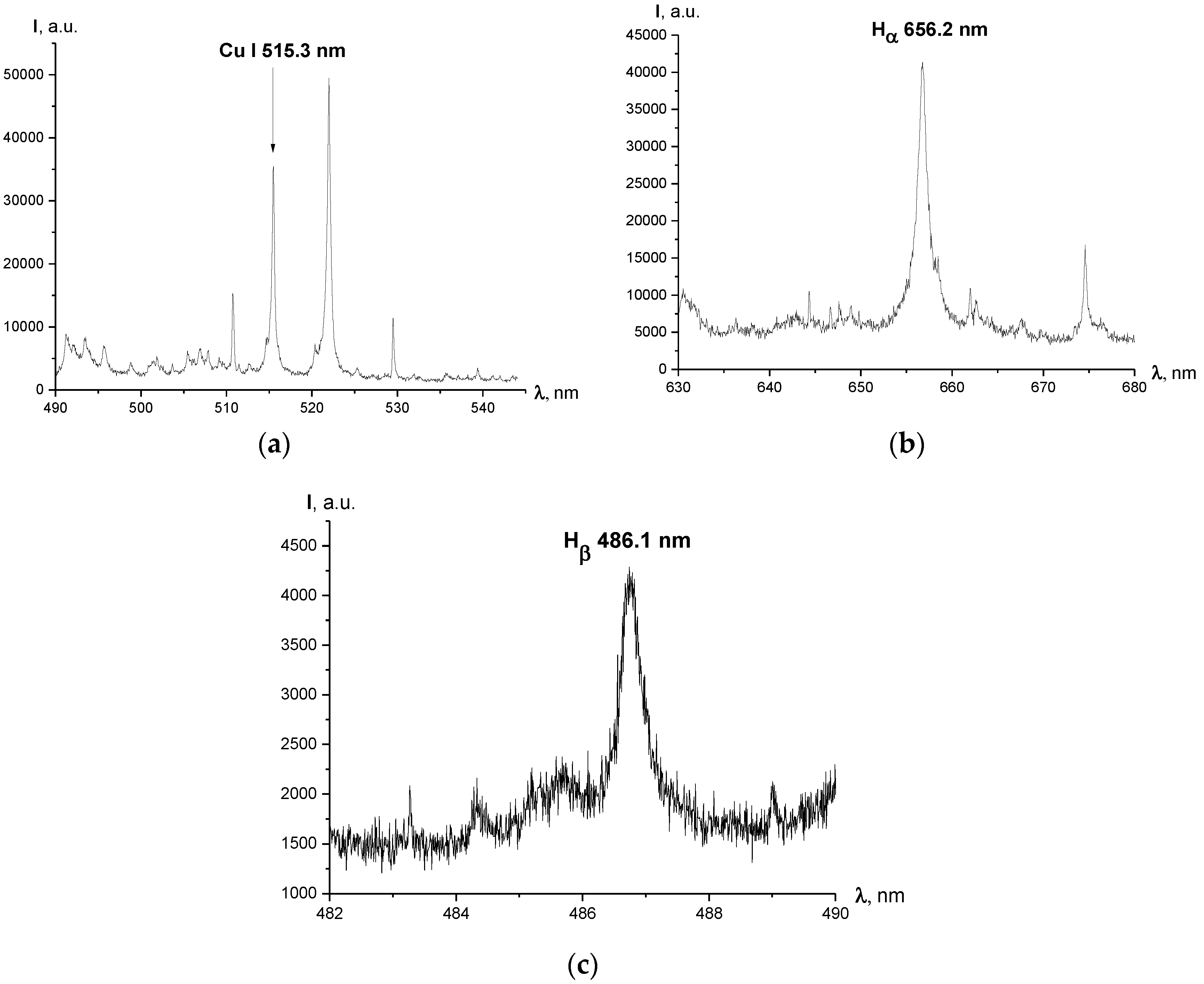
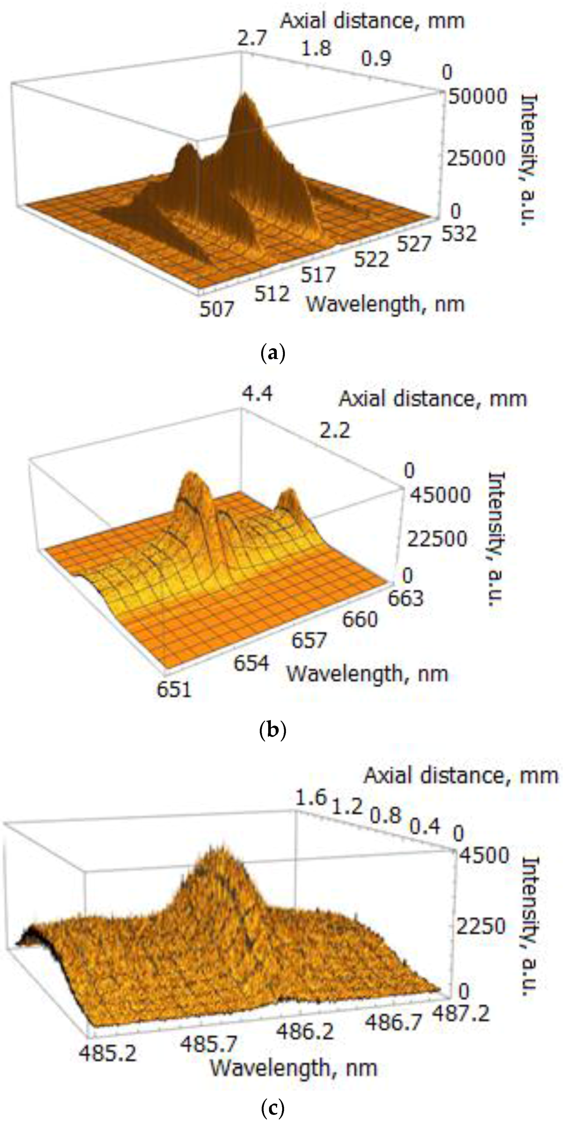
The typical spectra of hydrogen Balmer and Cu I lines registered for different experimental regimes are shown in Figure 2. Figure 3 presents the spatially resolved spectrum images of the selected lines. It should be noted that no trace of hydroxyl radicals (OH) was recorded throughout the experiments. The possible explanation for this can be the fact that electrohydraulic spark and arc discharges are quite different from the “partial” discharges, i.e., streamer and corona discharges. The current between electrodes is transferred here by electrons. Because of the relatively high breakdown electric field of water, a small interelectrode gap is necessary and the discharge current heats a small volume of plasma, which results in the generation of almost thermal plasma (the temperatures of the electron and the heavy particles are almost equal, as known from measurements on a water-stabilized plasma torch) [11]. Thermal plasmas pose a high risk of electrode erosion and are not very effective in the generation of radicals [18].
2.2.2. Broadening of Spectral Lines
The Stark broadening of the spectral lines is often used as a justified technique for the diagnosis of electron density (Ne), with applications not only in laboratory plasmas but also in astrophysical ones. This broadening is due to the collisions of the emitter with the charged particles in the surroundings of the emitter, according to the Stark effect. Stark broadening of the Balmer lines is the most popular approach to the determination of Ne since the broadening of the hydrogen lines, resulting from the linear Stark effect, is the strongest. These lines are, thus, those most sensitive to electron density variations. For the purposes of completeness and comparison, the electron density was also determined from the profile of Cu I 515.3 nm line, which is exposed to the quadratic Stark effect. In addition to Stark broadening, ideally, one should consider other broadening mechanisms, namely instrumental broadening, natural broadening, Doppler broadening, pressure broadening (resonance broadening, Van der Waals broadening), which have been reviewed in detail in [19,20]. More information about the broadening phenomena (physical phenomena, mathematical expressions of FWHMs, convolution procedure, etc.) are presented in Appendix A.
2.2.3. Line Broadening Values in Our Configuration
In our work, apparatus function has a Gaussian shape with a widths of 0.012 nm for the 300 lines/mm grating and 0.001 nm for the 1800 lines/mm grating. The order of magnitude of obtained wN values showed to be of ~10−5 nm and is negligible in comparison to the impact of other broadening mechanisms. Values of wR and wVdW are of the order of magnitude of ~10−3 nm and doesn’t vary significantly with the values of gas temperature Tg, and as well can be excluded out of calculations of the electron density. Therefore, profiles of the registered lines are fitted with a Voigt function, whereas the Gaussian part is presented by convolution of the instrumental and Doppler broadening, giving the values of 0.02–0.04 nm, and the Lorentzian part of the profile is considered to be only the Stark FWHM.
3. Results
3.1. Electron Density
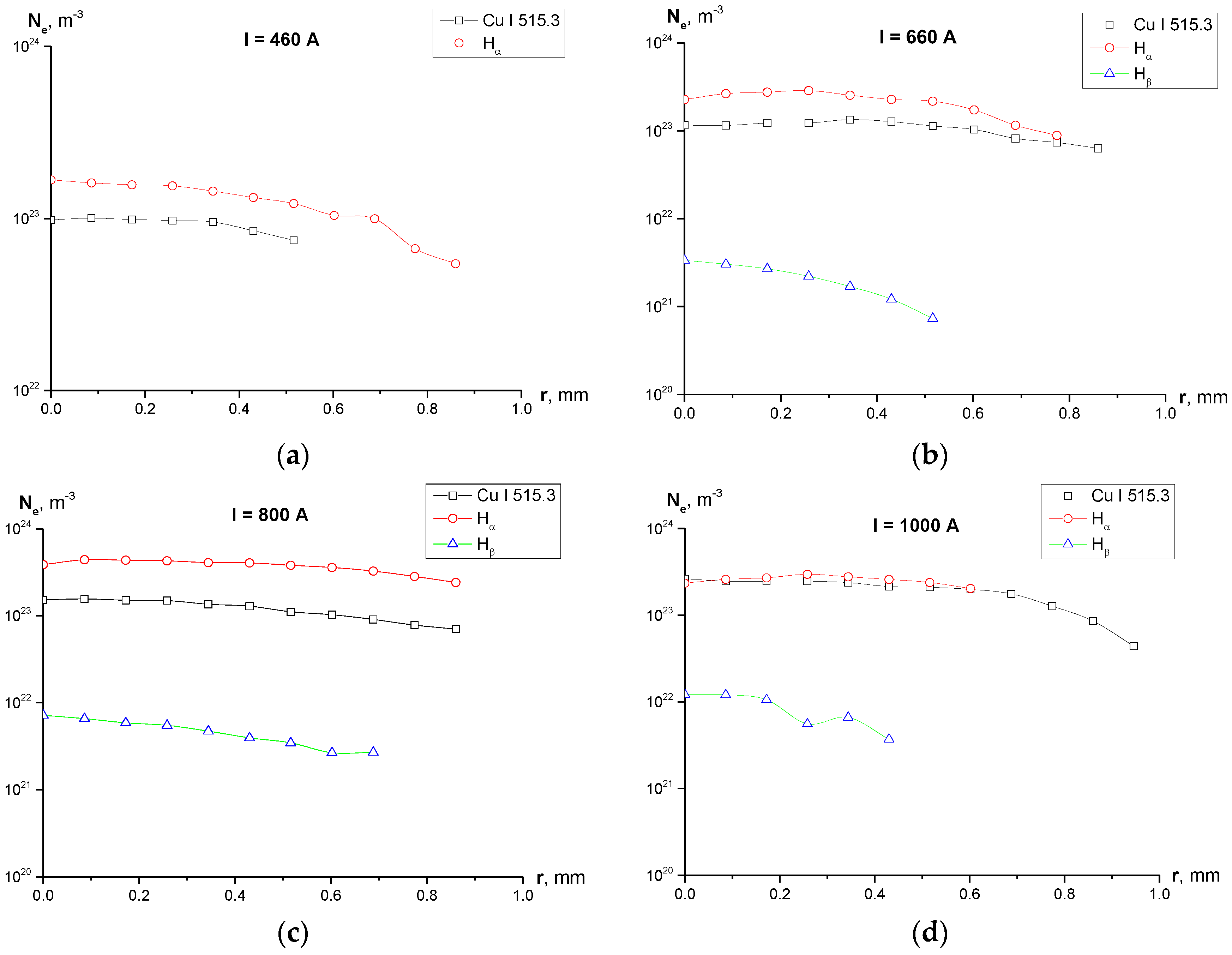
Line shapes and Voigt fit of the studied lines are shown in Figure 4. One can see in Figure 5 the radial profiles of electron number density for 1–2 mm diameter plasma. It can be noted that in Figure 4c there is a large uncertainty concerning the maximum of the line (between 875 a.u. and 975 a.u.) and, therefore, the FWHM. A higher maximum leads to a FWHM larger than 0.6 nm and therefore a larger electron density, but the Voigt fit was performed according to procedure recommended in [21] with the fixed Gaussian “contribution” into the line’s width, which resulted in the profile shown in Figure 4c.
3.2. High-Speed Imaging
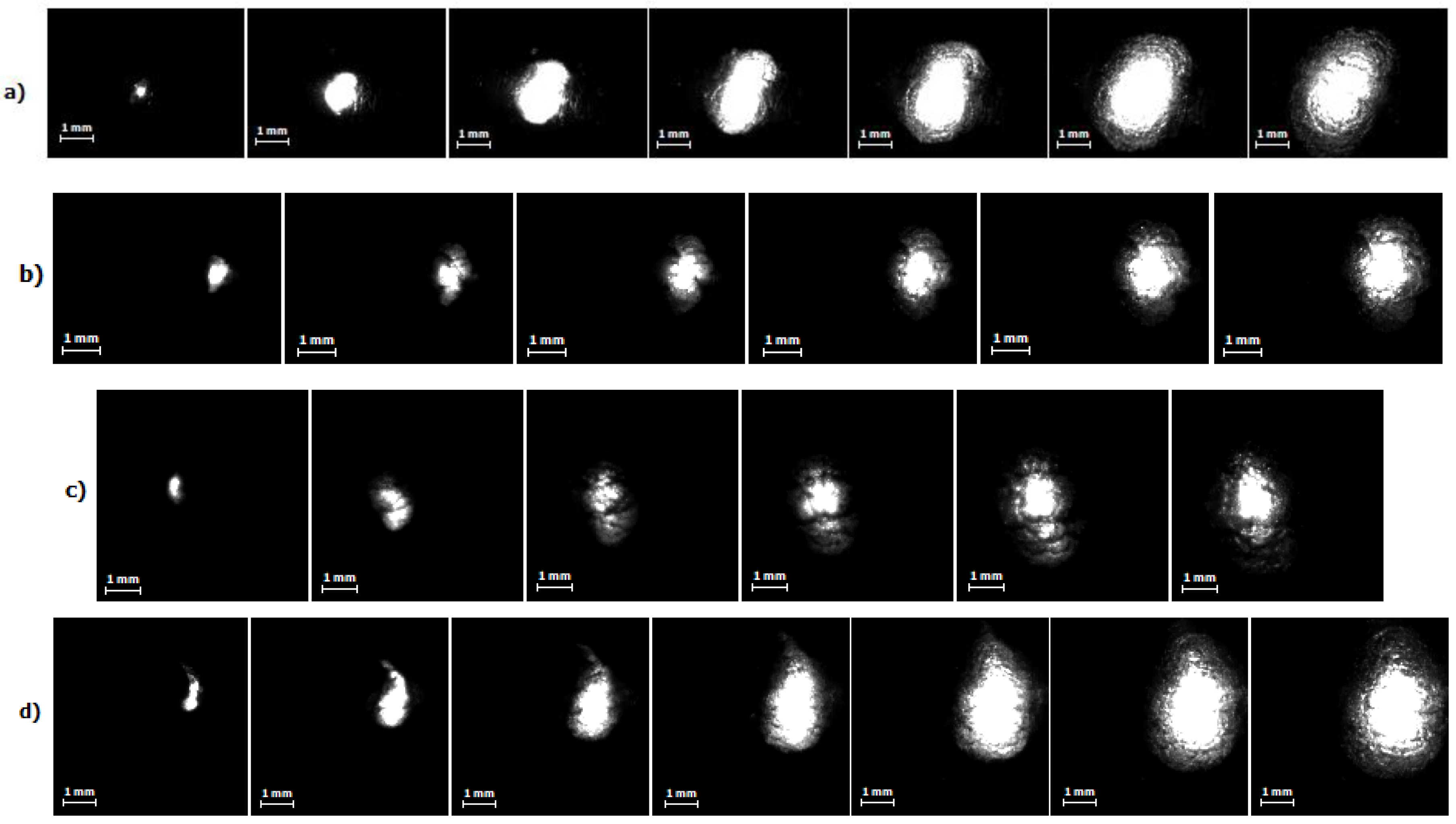
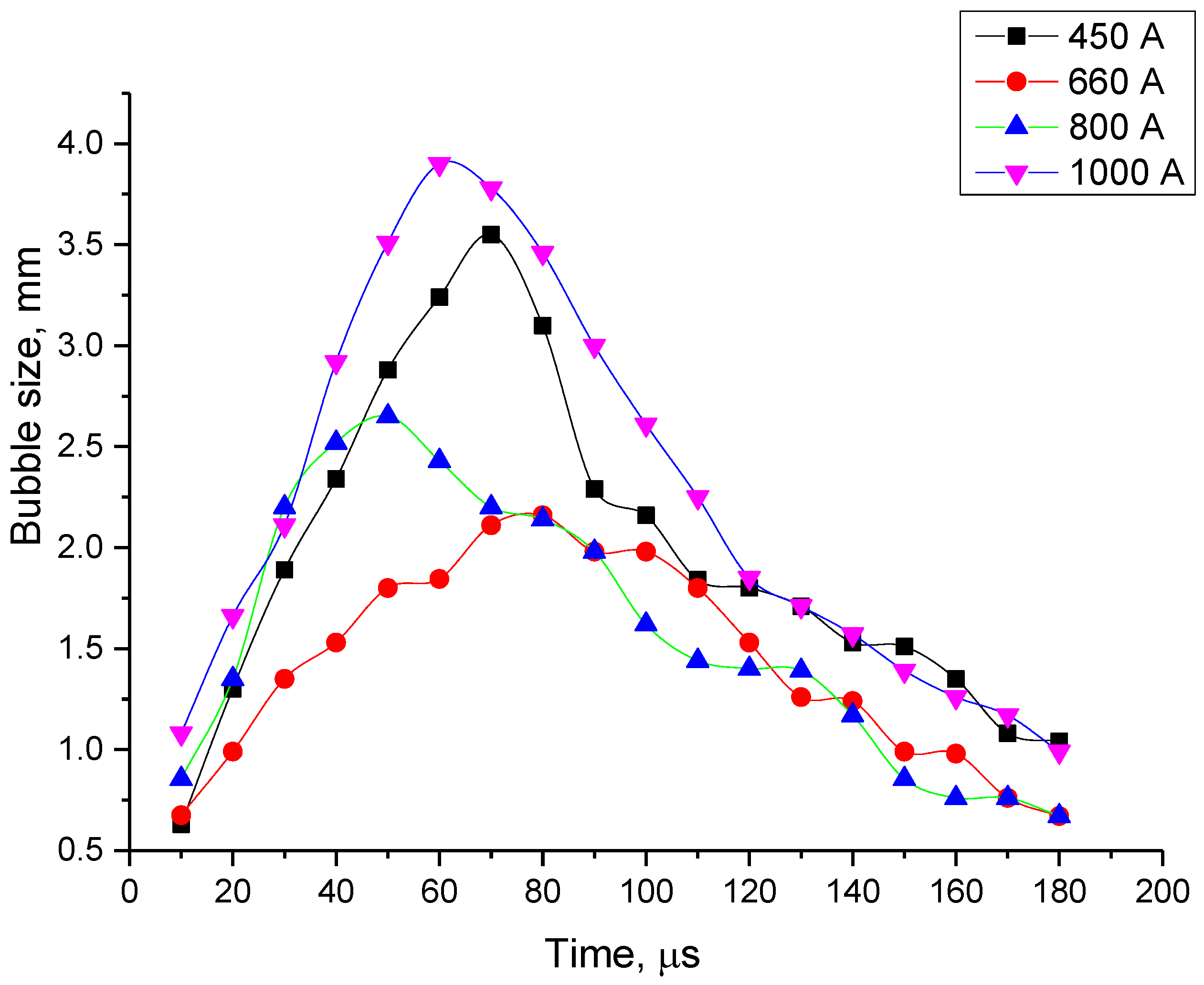
High-speed images of the discharge for different current regimes are presented in Figure 6, wherein the first image corresponds to a time about 10 µs after the pulse start. One can clearly see the bright spherical area corresponding to the discharge itself occurring into the bubble. Therefore, the information about the discharge and bubble development as a function of time and electrical parameters can be obtained. Figure 7 shows the images of evolution of bubble’s size up to its maximal diameter for every current regime studied in this work. Dependence of the bubble’s size on duration of the discharge for different current regimes is presented in Figure 8, and Figure 9 shows evolution of the bubble’s size depending on a discharge current for different regimes. The size of the bubble was estimated from the correspondence of 1 mm to number of pixels obtained from the photograph of the ruler made for scale. Figure 9 presents two values for the same current, the first half of the curve (the “upper” part) corresponds to rising current and the second half (the “lower” part, on the right side) to the falling current. This allows to see the bubble’s growth differs from its collapse.
3.3. Erosion of Electrodes
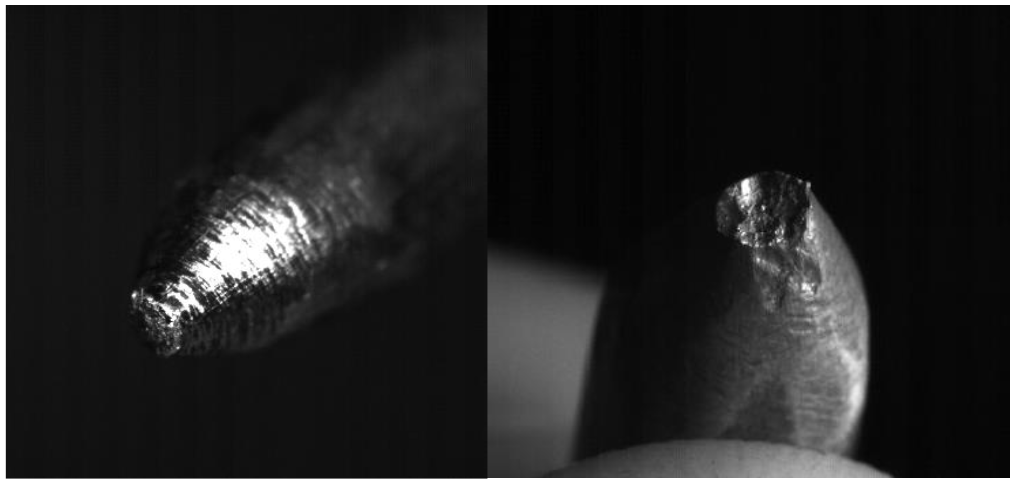
Measurements of erosion were performed by controlling the weights of cathode and anode before and after the experiments using digital scales with precision of 0.1 mg. Table 2 presents the data on electrodes’ erosion for current regime I = 450 A and I = 800 A, for comparison. Unfortunately, measurements of erosion were not carried out for current of 1 kA, since the electrode deformation after one pulse was so important that we needed to sharpen it again before the next pulse and the corresponding erosion was too low to get sufficient measurement accuracy.
4. Discussion and Conclusions
All the measurements and calculations performed within these experimental series allow us to make the following conclusion through the analysis of the results:
- For all the four current regimes studied in this work (I = 450 A, I = 660 A, I = 800 A and I = 1000 A), duration of the pulse in average shows to be 320–346 μs with the rise time of a current up to its maximum value of 90–100 μs (see Table 1). While raise time of a current up to its maximum value is the shortest for the current regime I = 450 A, the maximum bubble’s size is reached the fastest for the case of the current regime of I = 800 A, for which the current raise time is the longest. The only pattern that can be distinguished (see Figure 7 and Figure 9) is that the bubble reaches it maximum size not at the same time when the current value is on peak, but before that, maintaining its size more or less constant while current value equals to its maximum value for the given current regime. In order to be able to make any conclusions, more experiments must be performed, which will give the more reliable statistical data.
- The erosion does not change much for the different current regimes. Table 2 shows that for current of 800 A, which is approximately two times greater than the first current regime, increase of the eroded mass per pulse is ~20%. Erosion of anode shows to be greater than that of cathode (in our experiments anode is the moving electrode). This is consistent with the results obtained by other authors studying the submerged pulsed arc discharges [22], and may have one of the possible explanations that the energy dissipated in the anode is larger than in the cathode. As expected, the size of craters produced on the electrodes during arcing (Figure 10) increases with the measured erosion. The larger craters were formed on the anode where the erosion was larger.
- Calculation of the electron density shows (Figure 5) disagreement the values of Ne calculated using the Cu I 515.3 nm, Hα and Hβ lines. While Ne determined from the widths of Cu I 515.3 and Hα line are of the same order of magnitude for all the studied current regimes, values of Ne obtained from the width of Hβ line are by two orders of magnitude lower for cases of I = 660 and 800 A, and by one order of magnitude lower for the case of I = 1000 A.
Normally, the use of the Hα line can lead to the following problems:
- It could present a non-negligible self-absorption and it is necessary to evaluate how it affects the line broadening;
- It has a strong broadening by ion dynamics, an effect that can be evaluated by using some computational methods recently developed which allow us to simulate the profiles of the spectral lines [23].
Taking into account the fact that self-absorption effects were not considered in the present study, one can conclude that the inconsistency between the values of Ne is caused by overestimation of the Hα line width. However, at the same time, values of Ne obtained from Hα line and Cu I 515.3 nm line show good agreement leading to the conclusion that the suggested value of the electron temperature Te = 10,000 K and Ne ~1023 m−3 are close to the experimental values of the electron density and electron temperature in our discharge.
It was shown in [24] that the expression connecting the Stark width of Balmer lines with Ne, which has been derived from the Kepple–Griem theory (KG) [25], in case of use of Hα line, overestimates the electron density by about 80% with respect to the Ne obtained from the Hβ line. This overestimation is due to the KG theory not taking into account the influence of the ion dynamics on the spectral profiles of the Balmer series lines. Computational methods taking into consideration these ion dynamic effects have been developed, among them the Gigosos–Cardenoso model (GC) [26] permitting the use of a line different from Hβ for measuring the electron density, obtaining in this way the same value of density as the one obtained from Hβ.
Values of the FWHM of Hα and Hβ lines with the corresponding Ne and Te = 10,000 K for the case of μ = 0.9 (reduced perturber mass corresponding to the hydrogen emitter and any perturbing atom or ion) are showed in Table 3.
It can be seen from the Table 3 that in order to get the same Ne at Te = 10,000 K, FWHM of Hβ line must be between 3 and 4 times greater than that of Hα, while the experimentally obtained values of FWHM of Hβ line are around 2–6 times smaller than that of Hα. (see Table 4), which, to our beliefs, leads to the correspondingly lower values of the estimated Ne.
It can be seen from Table 3 and Table 4 that the obtained results of FWHM of Hα line are in the 30–33% agreement with the data given by GC in [23] in terms of Ne/FWHM ratio.
Therefore, the conclusion can be made that it is important to estimate the self-absorption of the Hα line in order to double-check the results. Moreover, other techniques for the electron density determination should be used to validate the obtained results, for instance, determination of the electron density from continuum radiation, or, for instance, technique proposed in [27].
Author Contributions
Anatoly Veklich and Yann Cressault set and planned and designed the whole outline of the presented work; Flavien Valensi, Tetiana Tmenova designed and assembled the experimental setup, and carried out the experiments described in this work with assistance of and Roman Venger; Tetiana Tmenova and Viacheslav Boretskij performed the analysis of the experimental results; Tmenova Tetiana wrote the paper.
Conflicts of Interest
The authors declare no conflict of interest.
Appendix A
Whenever the contribution of other broadening mechanisms compared to Stark broadening is not negligible, the deconvolution procedure must be employed to determine Stark width–ws, which is used to determine Ne from the comparison with theoretical widths at the same electron temperature (Te).
One should consider the following mechanisms contributing to the spectral line profile and width:
- Instrumental broadening;
- Natural broadening;
- Doppler broadening;
- Pressure broadening (resonance broadening, Van der Waals broadening).
The deconvolution of the various contributions in the line broadened profile can be carried out based on the fact that, in many cases, the experimentally measured line profiles can be fitted with the Voigt function which is the convolution of the two functions: Gaussian and Lorentzian with the full width at half maximum (FWHM) given by wG and wL. The FWHM of a Voigt profile can be represented through the combination of the Gauss and Lorentz components as follows [21]:
The broadening contributions with a Gaussian shape will lead to a profile with wG determined as:
Whereas for Lorentzian broadening components the final contribution to the line profile will also be Lorentzian, with FWHM determined as:
Appendix A.1. Instrumental Broadening
Instrumental broadening is important, in particular at low Ne and low emitter’s temperature when line profile is narrow, i.e., when Stark broadening is small or comparable with other broadening mechanisms. The standard practice to determine the apparatus profile of a spectrometer is to scan over a line whose intrinsic width is very small compared to the apparatus width so that the latter determines its shape. Typically, such narrow lines are obtained from low-pressure discharges, like Geissler tubes or hollow cathode lamps. The instrumental line shapes obtained with good spectrometers are usually approximately Gaussian profiles in particular central core which usually is being used for deconvolution procedure.
Appendix A.2. Natural Broadening
Natural broadening is a consequence of the Heisenberg uncertainty principle applied to the energies of the initial and the final states of the transition. The uncertainty on the transition frequency or wavelength translates into a Lorentzian line profile of FWHM, for transition between states n and m [19]:
where λnm is the wavelength of a spectral line corresponding to transition from an upper state n to the lower state m (in cm), Anu, Amu are the transition probabilities of transitions between the states n, m and any ‘allowed’ level u, correspondingly Natural broadening is largest when one of the two levels is dipole-coupled to the ground state. Even in this case, it is usually negligible (of the order of 10−4 nm). However, it may be of some importance for low electron density plasmas generated in low-pressure gas discharges. The values of the Einstein A coefficients for calculations were taken from [28].
Appendix A.3. Resonance Broadening
Resonance broadening occurs for transitions involving a level that is dipole-coupled to the ground state and can be derived from the following equation [19]:
where λ is the wavelength (in cm) of the observed radiation. Here, Na is the density of ground state particles which are the same species as the emitter, and gi and gk are the statistical weights of the upper and lower state; λR and fR are the wavelength and f-value (oscillator strength), respectively, of the resonance transition from level “R”. The level “R” is the upper or lower level of the observed transition, which happens also to be the upper level of a resonance transition to the ground state. Not all transitions involve such a level. The values of fR, gi and gk for calculations were taken from [28].
Appendix A.4. Van der Waals Broadening
Van der Waals broadening results from the dipole interaction of an excited atom with the induced dipole of a neutral ground-state atom of density Na. This is a short-range C6/r6 interaction. The full-width at half-maximum of the Lorentzian profile wVdW can be written as [19]:
where
is the difference of the squares of coordinate vectors (in a0 units) of the upper and lower level, and μ is the atom-perturber reduced mass in a.m.u. In the Coulomb approximation the values of and in (7) may be calculated from
where the square of effective quantum number is
where EH is the ionization potential of hydrogen (109,737.32 cm−1). Here is the ionization potential of the studied element and Ej is the energy of the upper or lower level of the transition.
Values of , the mean atomic polarizability of the neutral perturber, are tabulated for different elements in [29]. If the required value of is not tabulated, it can also be estimated from the expression given in [29]:
where EEXC is the energy of the first excited level of the perturber.
Van der Waals broadening causes a red wavelength shift which is two-third of the size of the width wVdW. In our case, we consider that discharge occurs at atmospheric pressure (or higher) in air with 1–2% of the hydrogen, similar to [30]. Therefore, value of presents a sum of atomic polarizabilities of air components (O, N, O2, N2, NO), and it was not taken from [29], but was calculated using Equation (A8). Mean atom-perturber reduced mass μ is taken to be equal to one (reduced perturber mass corresponding to the hydrogen emitter and any perturbing atom or ion).
Appendix A.5. Doppler Broadening
The relative motion of an emitter to the detector leads to a shifted line. In plasma with gas temperature Tg the line profile due to the presence of Doppler effects can be well described by a Gaussian profile with a FWHM (nm):
where k is the Boltzmann constant (unit: J K−1) and Tg the gas temperature in K, and ma–the mass of the emitter (a.m.u.).
Appendix A.6. Stark Broadening
The analysis of Stark-broadened spectral-line profiles is one of the most common methods of plasma diagnosis from the beginning of the sixties. The shape of these profiles depends heavily on the density of charged particles surrounding the emitter. This dependence is especially important in hydrogen and hydrogenic ions, since in those elements a linear Stark effect takes place. As a consequence, Stark-broadening measurements have become one of the most widely used techniques when plasma electron density is to be determined. On the other hand, accurate knowledge of the shapes of the line profiles are mandatory in order to determine the opacity spectral distribution. These kind of diagnostics play a key role in astrophysics, where active spectroscopy is not possible.
To this end, profile tables of hydrogen Stark broadening have been in use since the beginning of the seventies [20,31]. The calculations leading to these tables were made in the framework of a plasma model in which it is assumed that the broadening of the lines can be computed as a sum of the contributions of all the collisions of a statistical ensemble of quasi-independent charged particles with the emitting atom. Depending on the speed of the perturbing particles, two different approximations were considered in order to simplify the computation of the contribution of each of the two different broadening mechanisms which are taken into account: it is assumed that the highly mobile electrons are responsible for sudden variations in the phase of the emitted wave–impact regime, while the heavier and slower ions generate electric fields which can be considered constant along the life of a typical emission–quasistatic regime.
The admissibility of this approximation seemed to be well secured for typical laboratory plasmas [20], and for that reason theoretical research in the field has concentrated mainly on electron broadening. The greater was the surprise when Kelleher and Wiese [32] and Wiese et al. [33] proved experimentally that the central parts of the first Balmer lines depend markedly on the reduced mass of the radiating atom-perturbing ion pair.
While these experimental results were obtained, other Stark-broadening calculation methods were developed [26,34].
Both the linear and the quadratic Stark effects are encountered in spectroscopy. However, only the hydrogen atom and H-like ions exhibit the linear Stark effect, whereas all other atoms exhibit the quadratic Stark effect. In the case of linear Stark effect, the relation between electron density and the line width can be expressed as a simple relation (static ion approximation) [35], being extremely convenient for the estimation of order of magnitude of the electron density value:
where wS is the FWHM of a Lorentzian contribution to the overall line profile and the parameter C(Ne,Te) depends (only weakly) on Ne and Te, which can normally be treated as being constant. The constant C for H Balmer lines is available in the literature [35]. Usually, the first choice for the electron density determination is Hβ line (with an error of 5%) [35] because of its large intensity and sufficiently large line broadening, which can be measured precisely using spectrometer of moderate resolution. The possibility of self-absorption in this case is relatively small. The second best choice among the Balmer series is the Hϒ line. The Hα line is suitable in the cases where the electron density is not too high (Ne ~1017 cm−3), because at higher electron densities this strong line is quite susceptible to self-absorption, which severely distorts the line profile.
In the case of non-H-like atoms, where the quadratic Stark effect is dominant, the relation between the electron density and the line width is [35]:
The first term in the brackets gives the contribution from the electron broadening, and the second term stems from ion broadening. Here w is the electron impact parameter at Ne = 1016 cm−3, and α is the ion broadening parameter. These parameters can be found easily from the literature [35]. Since the second term after opening the brackets in Equation (A13) is normally small, so the expression reduces to
It has been reported in [36] that the electron density derived from the Hβ line and Hϒ line data were in good agreement with each other, while the electron density estimated from the Hα line is not purely Stark broadened. The additional broadening might be due to the onset of self-absorption.
In this work, values of electron density were obtained using Hβ, Hα lines from the following equations presented in [26], which takes into account the ion dynamic effects:
Electron density for Cu I 515.3 nm line is obtained from the linear interpolation from the table presented in [37], whereas the theoretical and experimental Stark widths of Cu I lines are listed for Ne = 1017 cm−3 and Te = 10,000 K. These values were assumed as parameters for the estimations presented in this work.
References
- Ternes, T.A.; Hirsch, R. Occurrence and behavior of X-ray contrast media in sewage facilities and the aquatic environment. Environ. Sci. Technol. 2000, 34, 2741–2748. [Google Scholar] [CrossRef]
- Dunnick, J.K.; Melnick, R.L. Assessment of the carcinogenic potential of chlorinated water: Experimental studies of chlorine, chloramine, and trihalomethanes. J. Natl. Cancer Inst. 1993, 85, 817–822. [Google Scholar] [CrossRef] [PubMed]
- Ternes, T.A.; Stueber, J.; Herrmann, N.; McDowell, D.; Ried, A.; Kampmann, M.; Teiser, B. Ozonation: A tool for removal of pharmaceuticals, contrast media and musk fragrances from wastewater. Water Res. 2003, 37, 1976–1982. [Google Scholar] [CrossRef]
- Babaeva, N.Y.; Kushner, M.J. Streamer Branching: The Role of Inhomogeneities and Bubbles. IEEE Trans Plasma Sci. 2008, 36, 892–893. [Google Scholar] [CrossRef]
- Bruggeman, P.; Leys, C. Non-thermal plasmas in and in contact with liquids. Top. Rev. J. Phys. D Appl. Phys. 2009, 42, 1–28. [Google Scholar] [CrossRef]
- Clements, J.S.; Sato, M.; Davis, R.H. Preliminary investigation of prebreakdown phenomena and chemical reactions using a pulsed high-voltage discharge in water. IEEE Trans. Ind. Appl. 1987, 23, 224–235. [Google Scholar] [CrossRef]
- Li, O.L.H.; Chang, J.S.; Guo, Y. Pulsed arc electrohydraulic discharge characteristics, plasma parameters, and optical emission during contaminated pond water treatments. IEEE Electr. Insul. Mag. 2011, 27. [Google Scholar] [CrossRef]
- Sunka, P. Pulse electrical discharges in water and their applications. Phys. Plasmas 2001, 8, 2587–2594. [Google Scholar] [CrossRef]
- Akiyama, H.; Sakugawa, T.; Namihira, T. Industrial applications of pulsed power technology. IEEE Trans. Dielectr. Electr. Insul. 2007, 14, 1051–1064. [Google Scholar] [CrossRef] [Green Version]
- Bluhm, H.; Frey, W.; Giese, H. Application of pulsed HV discharges to material fragmentation and recycling. IEEE Trans. Dielectr. Electr. Insul. 2000, 7, 625–636. [Google Scholar] [CrossRef]
- Locke, B.R.; Sato, M.; Sunka, P.; Hoffmann, M.R.; Chang, J.S. Electrohydraulic discharge and nonthermal plasma for water treatment. Ind. Eng. Chem. Res. 2006, 45, 882–905. [Google Scholar] [CrossRef]
- Chen, Q.; Li, J.; Li, Y. A review of plasma–liquid interactions for nanomaterial synthesis. J. Phys. D Appl. Phys. 2015, 48, 424005. [Google Scholar] [CrossRef]
- Tmenova, T.A.; Veklich, A.N.; Boretskij, V.F.; Cressault, Y.; Valensi, F.; Lopatko, K.G.; Aftandilyants, Y.G. Optical emission spectroscopy of plasma of underwater electric spark discharges between metal granules. Probl. Atomic Sci. Technol. 2017, 1, 132–135. [Google Scholar]
- Cressault, Y.; Teulet, P.; Gleizes, A.; Lopatko, K.; Melnichuk, M.; Aftandilyants, Y.; Gonchar, E.; Boretskij, V.; Veklich, A. Peculiarities of metal nanoparticles generation by underwater discharges for biological applications. In Proceedings of the XXXI International Conference on Phenomena in Ionized Gases, Granada, Spain, 14–19 July 2013. [Google Scholar]
- Lopatko, K.G.; Aftandіlyants, I.G.; Kalenska, S.M. Colloidal Solution of Metal. Ukrainian Patent No. 38459, 12 January 2009. [Google Scholar]
- Xiu, Z.; Zhang, Q.; Puppala, H.L.; Colvin, V.L.; Alvarez, P.J. Negligible Particle-Specific Antibacterial Activity of Silver Nanoparticles. Nano Lett. 2012, 12, 4271. [Google Scholar] [CrossRef] [PubMed]
- Babich, I.L.; Boretskij, V.F.; Veklich, A.N.; Semenyshyn, R.V. Spectroscopic data and Stark broadening of Cu I and Ag I spectral lines: Selection and analysis. Adv. Space Res. 2014, 54, 1254–1263. [Google Scholar] [CrossRef]
- Yang, Y.; Cho, I.Y.; Fridman, A. Plasma Discharge in Liquid: Water Treatment and Applications; CRC Press: Boca Raton, FL, USA, 2012; pp. 10–29. [Google Scholar]
- Konjević, N. Plasma broadening and shifting of non-hydrogenic spectral lines: Present status and applications. Phys. Rep. 1999, 316, 339–401. [Google Scholar] [CrossRef]
- Griem, H.R. Spectral Line Broadening by Plasmas; Academic Press: New York, NY, USA, 1974. [Google Scholar]
- Konjević, N.; Ivković, M.; Sakan, N. Hydrogen Balmer lines for low electron number density plasma diagnostics. Spectrochim. Acta B At. Spectrosc. 2012, 76, 12–26. [Google Scholar] [CrossRef]
- Parkansky, N.; Glikman, L.; Beilis, I.I.; Alterkop, B.; Boxman, R.L.; Gindin, D. W–C electrode erosion in a pulsed arc submerged in liquid. Plasma Chem. Plasma Process. 2007, 27, 789–797. [Google Scholar] [CrossRef]
- Gigosos, M.A.; Cardeñoso, V. New plasma diagnosis tables of hydrogen Stark broadening including ion dynamics. J. Phys. B At. Mol. Opt. Phys. 1996, 29, 4795. [Google Scholar] [CrossRef]
- Luque, J.M.; Calzada, M.D.; Sáez, M. Experimental research into the influence of ion dynamics when measuring the electron density from the Stark broadening of the Hα and Hβ lines. J. Phys. B At. Mol. Opt. Phys. 2003, 36, 1573. [Google Scholar] [CrossRef]
- Kepple, P.; Griem, H.R. Improved Stark Profile Calculations for the Hydrogen Lines Hα, Hβ, Hγ, and Hδ. Phys. Rev. 1968, 173, 317. [Google Scholar] [CrossRef]
- Gigosos, M.A.; Gonzalez, M.A.; Cardenoso, V. Computer simulated Balmer-alpha,-beta and -gamma Stark line profiles for non-equilibrium plasmas diagnostics. Spectrochim. Acta B 2003, 58, 1489–1504. [Google Scholar] [CrossRef]
- Torres, J.; Carabano, O.; Fernández, M.; Rubio, S.; Álvarez, R.; Rodero, A.; Lao, C.; Quintero, M.C.; Gamero, A.; Sola, A. The stark-crossing method for the simultaneous determination of the electron temperature and density in plasmas. J. Phys. Conf. Ser. 2006, 44, 70–79. [Google Scholar] [CrossRef]
- Wiese, W.L.; Smith, M.W.; Glennon, B.M. Atomic Transition Probabilities: Hydrogen through Neon; US Department of Commerce, National Bureau of Standards: Washington, DC, USA, 1996; Voloume 1, pp. 1–8.
- Allen, C.W. Allen’s Astrophysical Quantities, 4th ed.; Cox, A.N., Ed.; Springer: New York, NY, USA, 2015; pp. 27–79. [Google Scholar]
- Nikiforov, A.Y.; Leys, C.; Li, L.; Nemcova, L.; Krcma, F. Physical properties and chemical efficiency of an underwater dc discharge generated in He, Ar, N2 and air bubbles. Plasma Sources Sci. Technol. 2011, 20, 034008. [Google Scholar] [CrossRef]
- Vidal, C.R.; Cooper, J.; Smith, E.W. Hydrogen Stark-broadening tables. Astrophys. J. Suppl. Ser. 1973, 25, 37. [Google Scholar] [CrossRef]
- Kelleher, D.E.; Wiese, W.L. Observation of ion motion in hydrogen Stark profiles. Phys. Rev. Lett. 1973, 31, 1431. [Google Scholar] [CrossRef]
- Wiese, W.L.; Kelleher, D.E.; Helbig, V. Variations in Balmer-line Stark profiles with atom-ion reduced mass. Phys. Rev. A 1975, 11, 1854. [Google Scholar] [CrossRef]
- Seidel, J. Hydrogen Stark broadening by different kinds of model microfields. Z. Naturforsch. A 1980, 35, 679–689. [Google Scholar] [CrossRef]
- Griem, H.R. Plasma Spectroscopy; McGraw-Hill Book Company: New York, NY, USA, 1964. [Google Scholar]
- Samek, O.; Beddows, D.C.; Kaiser, J.; Kukhlevsky, S.V.; Liska, M.; Telle, H.H.; Young, J. Application of laser-induced breakdown spectroscopy to in situ analysis of liquid samples. Opt. Eng. 2000, 39, 2248–2262. [Google Scholar]
- Konjević, R.; Konjević, N. Stark broadening and shift of neutral copper spectral lines. Fizika 1986, 18, 327–335. [Google Scholar]
Figure 1.
Experimental setup for the underwater arc discharge generation.
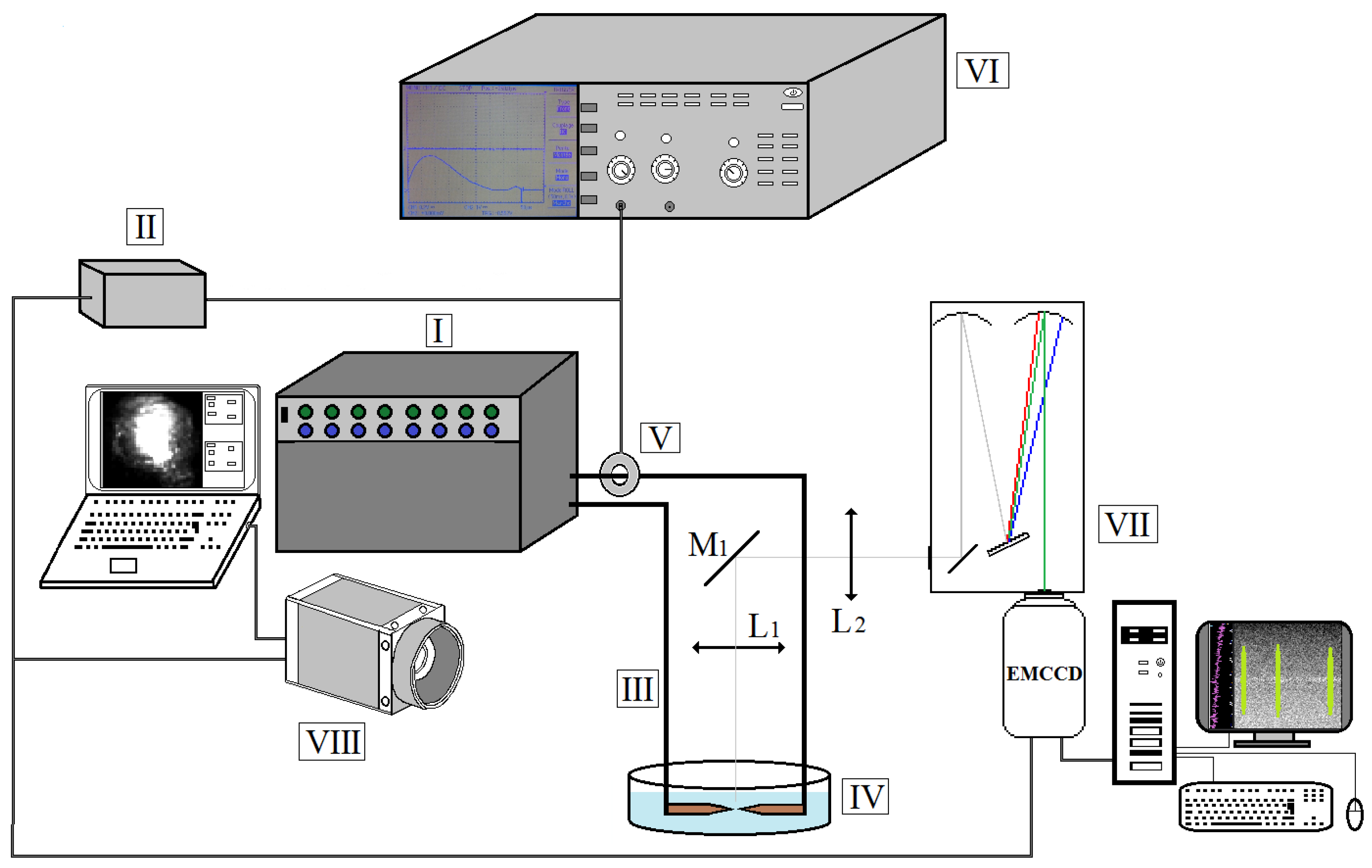
Figure 2.
Typical spectra obtained throughout the experiments (cross-section of the arc halfway between the electrodes); exposure time of the EMCCD τ = 200 μs: (a) spectrum of Cu I lines registered for I = 450 A, central wavelength λ = 515.0 nm, grating 300 lines/mm; (b) Hα line registered for I = 450 A, central wavelength λ = 616.5 nm, grating 300 lines/mm; (c) Hβ line registered for I = 660 A, central wavelength λ = 486.1 nm (Hβ line wasn’t registered for the current regime of 450 A due to its low intensity), grating 1800 lines/mm.

Figure 3.
Spatially resolved spectrum images of the selected lines; exposure time of the EMCCD τ = 200 μs: (a) spectrum of Cu I lines registered for I = 400 A; (b) Hα line registered for I = 400 A; (c) Hβ line registered for I = 660 A.
Figure 3.
Spatially resolved spectrum images of the selected lines; exposure time of the EMCCD τ = 200 μs: (a) spectrum of Cu I lines registered for I = 400 A; (b) Hα line registered for I = 400 A; (c) Hβ line registered for I = 660 A.

Figure 4.
Line profiles and Voigt fit of the registered lines for current regime I = 1000 A, radial position r = 0 mm (discharge axis): (a) Cu I 515.3 nm line; (b) Hα line; (c) Hβ line.
Figure 4.
Line profiles and Voigt fit of the registered lines for current regime I = 1000 A, radial position r = 0 mm (discharge axis): (a) Cu I 515.3 nm line; (b) Hα line; (c) Hβ line.
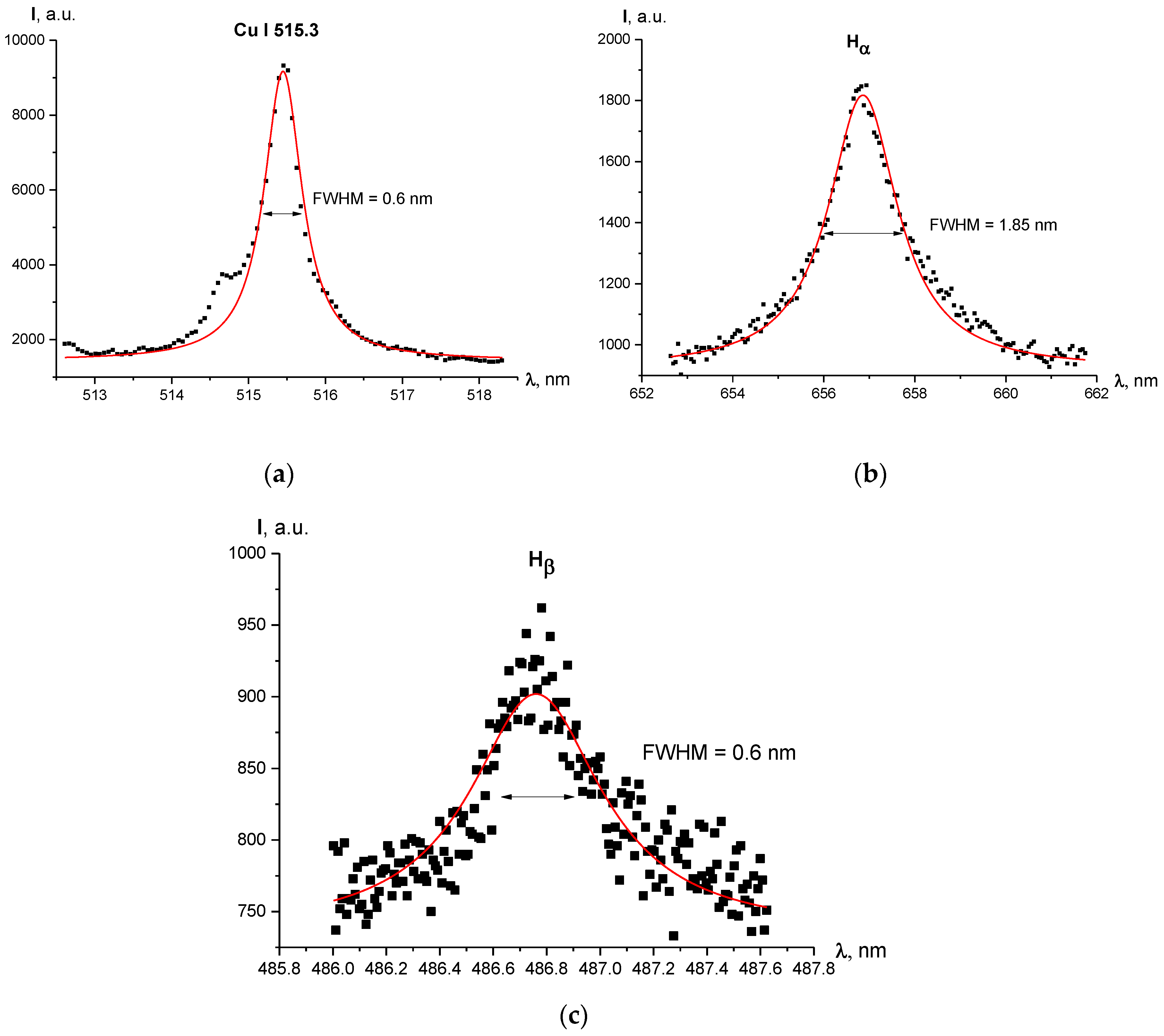
Figure 5.
Radial profiles of the electron density calculated using broadening of the selected registered lines for different experimental current regimes: (a) I = 450 A, Ne calculated using Cu I 515.3 nm line and Hα line; (Hβ line was not registered for this regime); (b) I = 660 A, Ne calculated using Cu I 515.3 nm, Hα and Hβ lines; (c) I = 800 A, Ne calculated using Cu I 515.3 nm, Hα and Hβ lines; (d) I = 1000 A, Ne calculated using Cu I 515.3 nm, Hα and Hβ lines.

Figure 6.
High-speed image recording of the discharge for different current regimes: (a) I = 450 A, time interval between presented frames–60 μs, image resolution–128 × 96 px, frame rate–100,000 fps; (b) I = 660 A, time interval between presented frames–60 μs; image resolution–128 × 96 px, frame rate–100,000 fps; (c) I = 800 A, time interval between presented frames–65 μs; image resolution–128 × 128 px, frame rate–75,000 fps; (d) I = 1000 A, time interval between presented frames–65 μs; image resolution–128 × 128 px, frame rate–75,000 fps.
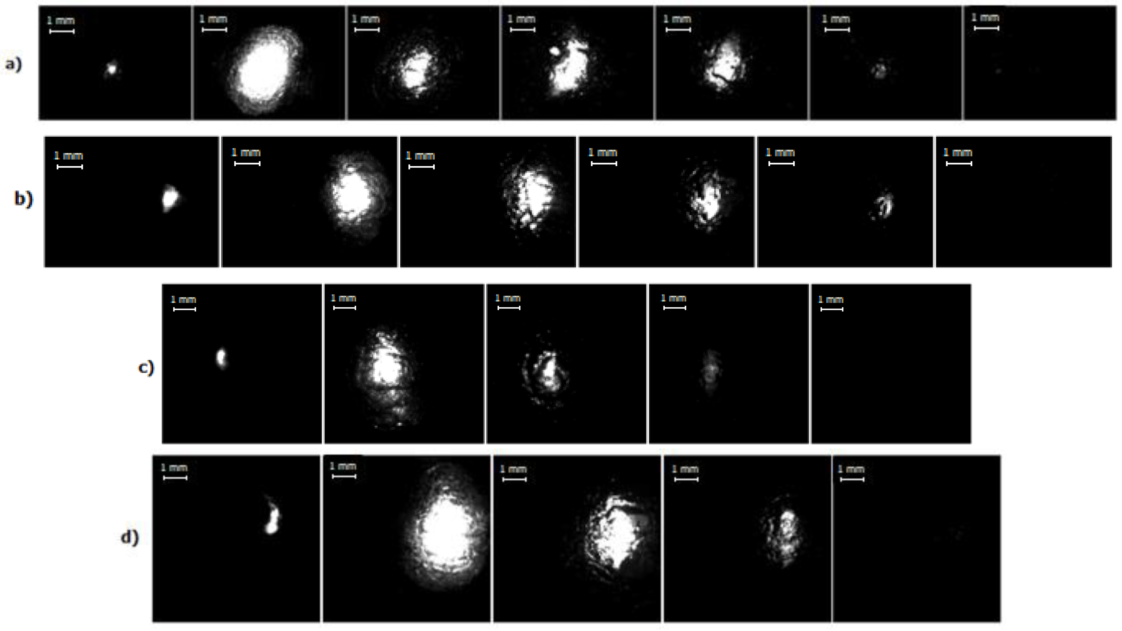
Figure 7.
High-speed imaging of the discharge and bubble size development up to the maximal size for different current regimes: (a) I = 450 A, time interval between presented frames–60 μs, image resolution–128 × 96 px, frame rate–100,000 fps; (b) I = 660 A, time interval between presented frames–60 μs; image resolution–128 × 96 px, frame rate–100,000 fps; (c) I = 800 A, time interval between presented frames–65 μs; image resolution–128 × 128 px, frame rate–75,000 fps; (d) I = 1000 A, time interval between presented frames–65 μs; image resolution–128 × 128 px, frame rate–75,000 fps.

Figure 8.
Time evolution of a bubble’s size for different values of maximal current.

Figure 9.
Evolution of the bubble’s size depending on a discharge current (its evolution in time within one pulse) for different values of maximal current: (a) for maximal current of 450 A; (b) for maximal current of 660 A; (c) for maximal current of 800 A; (d) for maximal current of 1000 A.
Figure 9.
Evolution of the bubble’s size depending on a discharge current (its evolution in time within one pulse) for different values of maximal current: (a) for maximal current of 450 A; (b) for maximal current of 660 A; (c) for maximal current of 800 A; (d) for maximal current of 1000 A.
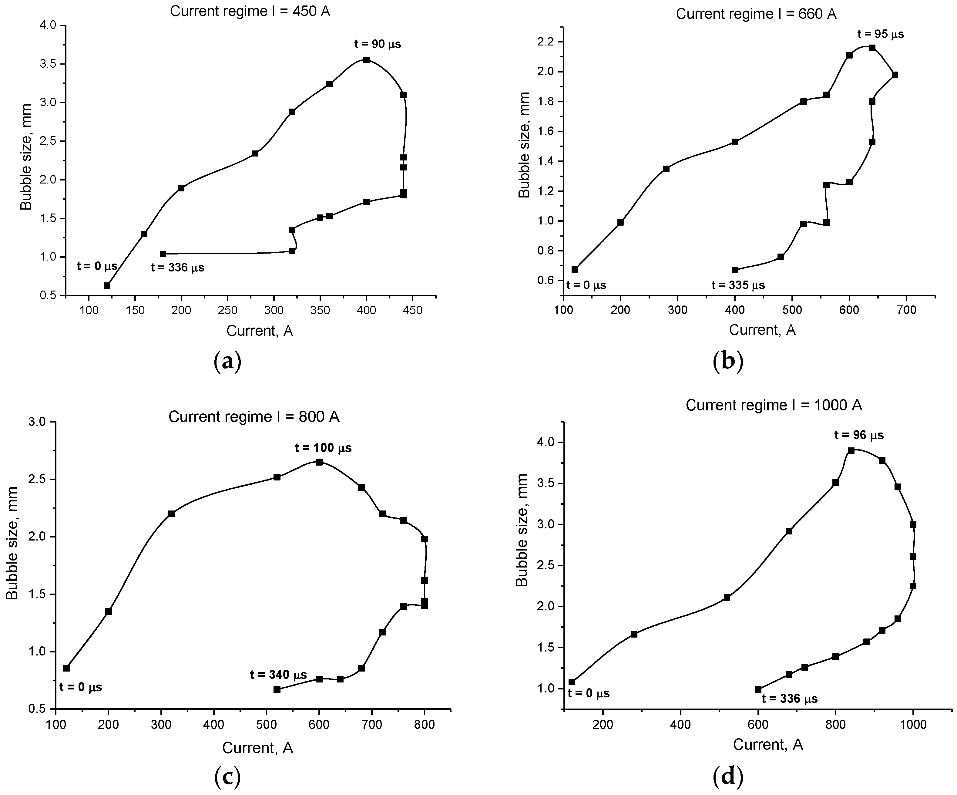
Figure 10.
Photographs of the cathode (left) and anode (right) after the series of 15 experiments for I = 450 A. Diameter of both electrodes is 6 mm.
Figure 10.
Photographs of the cathode (left) and anode (right) after the series of 15 experiments for I = 450 A. Diameter of both electrodes is 6 mm.

Table 1.
Electric parameters of the experimental setup corresponding to different current regimes (per pulse).
Table 1.
Electric parameters of the experimental setup corresponding to different current regimes (per pulse).
| Idisch, A 1 | Uc, V 2 | P, kW | τraise, μs 3 | τdisch, μs 4 | τtotal, μs |
|---|---|---|---|---|---|
| 450 | 120 | 54 | 90 | 230 | 320 |
| 660 | 150 | 100 | 95 | 240 | 335 |
| 800 | 180 | 146 | 100 | 240 | 340 |
| 1000 | 220 | 217 | 96 | 240 | 336 |
Notes: 1 Idisch corresponds to the peak value of the current; 2 Uc corresponds to the load capacitor voltage; 3 τraise corresponds to the duration of the current raise up to its maximum value; 4 τdisch corresponds to the duration of the current decrease.
Table 2.
Erosion of the copper electrodes after the carried out experiments.
| Current (I, A) | Number of Consecutive Pulses | Erosion of Anode, g | Erosion of Cathode, g | Total Erosion, g | Erosion Per Pulse (g/Pulse) |
|---|---|---|---|---|---|
| 450 | 15 | 0.0038 | 0.0005 | 0.0043 | 0.00028 |
| 800 | 15 | 0.004 | 0.0012 | 0.0052 | 0.00034 |
| logNe (m−3) | FWHM (nm) for Hα | FWHM (nm) for Hβ |
|---|---|---|
| 20.00 | 0.0142 | 0.0424 |
| 20.33 | 0.0244 | 0.0741 |
| 20.67 | 0.0404 | 0.129 |
| 21.00 | 0.064 | 0.217 |
| 21.33 | 0.102 | 0.361 |
| 21.67 | 0.16 | 0.601 |
| 22.00 | 0.25 | 0.999 |
| 22.33 | 0.393 | 1.67 |
| 22.67 | 0.621 | 2.80 |
| 23.00 | 1.01 | 4.70 |
| 23.33 | 1.68 | 7.77 |
| 23.67 | 2.84 | 1.27 |
| 24.00 | 4.86 | 2.05 |
| 24.33 | 8.31 | 3.25 |
Table 4.
Experimentally obtained values of FWHM of Hα and Hβ lines (in nm).
| Line | FWHM (nm) at I = 660 A | FWHM (nm) at I = 800 A | FWHM (nm) at I = 1000 A | Average log Ne (m−3) |
|---|---|---|---|---|
| Hα | 1.13 | 2.60 | 2.40 | 23.36 |
| Hβ | 0.40 | 0.39 | 0.57 | 21.51 |
© 2017 by the authors. Licensee MDPI, Basel, Switzerland. This article is an open access article distributed under the terms and conditions of the Creative Commons Attribution (CC BY) license (http://creativecommons.org/licenses/by/4.0/).
Share and Cite
MDPI and ACS Style
Venger, R.; Tmenova, T.; Valensi, F.; Veklich, A.; Cressault, Y.; Boretskij, V. Detailed Investigation of the Electric Discharge Plasma between Copper Electrodes Immersed into Water. Atoms 2017, 5, 40. https://doi.org/10.3390/atoms5040040
AMA Style
Venger R, Tmenova T, Valensi F, Veklich A, Cressault Y, Boretskij V. Detailed Investigation of the Electric Discharge Plasma between Copper Electrodes Immersed into Water. Atoms. 2017; 5(4):40. https://doi.org/10.3390/atoms5040040
Chicago/Turabian StyleVenger, Roman, Tetiana Tmenova, Flavien Valensi, Anatoly Veklich, Yann Cressault, and Viacheslav Boretskij. 2017. "Detailed Investigation of the Electric Discharge Plasma between Copper Electrodes Immersed into Water" Atoms 5, no. 4: 40. https://doi.org/10.3390/atoms5040040
Note that from the first issue of 2016, this journal uses article numbers instead of page numbers. See further details here.