High Temperature Optical Spectra of Diatomic Molecules at Local Thermodynamic Equilibrium

Abstract

In the paper, several theoretical approaches to the determination of the reduced absorption and emission coefficients under local thermodynamic equilibrium conditions were exposed and discussed. The full quantum-mechanical procedure based on the Fourier grid Hamiltonian method was numerically robust but time consuming. In that method, all transitions between the bound, free, and quasi-bound states were treated as bound–bound transitions. The semi-classical method assumed continuous energies of ro-vibrational states, so it did not give the ro-vibrational structure of the molecular bands. That approach neglected the effects of turning points but agreed with the averaged-out quantum-mechanical spectra and it was computer time efficient. In the semi-quantum approximation, summing over the rotational quantum number J was done analytically using the classical Franck–Condon principle and the stationary–phase approximation and its consumption of computer time was lower by a few orders of magnitude than the case of the full quantum-mechanical approach. The approximation described well the vibrational but not the rotational structure of the molecular bands. All the above methods were compared and discussed in the case of a visible and near infrared spectrum of LiHe, Li₂, and Cs₂ molecules in the high temperature range.

1. Introduction

Numerical simulations of the absorption and emission spectra of diatomic molecules provide efficient tools for checking the accuracy of molecular electronic structure calculations and diagnostics of vapors at high temperatures. To obtain valuable theoretical knowledge of the molecular spectra and pressure broadened atomic line profiles, one needs the precise molecular potential curves and transition dipole moments, as well as a correct and time-efficient theoretical spectral simulation method.

Theoretical spectra as functions of temperature and density enable interpretations of the observed spectra of gases in laboratory conditions, and the Earth or stellar atmosphere enables their temperature and number density determination. To do that in the theoretical spectra, simulation temperature and number density are changing as parameters in an iterative procedure to obtain the best agreement with the experimental spectra. Such a procedure for temperature and number density determination is time consuming. That is why we paid special attention in this paper to the numerical time-efficiency of the theoretical approaches described.

This article is organized as follows. The basic expressions for the reduced absorption and emission coefficients and their mutual relationship at the thermodynamic equilibrium are defined in Section 2. Several methods of spectral profile calculation are explained in Section 3. In Section 3.1, we discussed the semi-classical approach where the motion of atoms in a molecule is described by classical trajectory and the energies of bound and free ro-vibrational states are continuous. Here we suggested a new form of the generalized uniform Airy approximation of spectra (relations in Equations (22) and (23)) it was suitable for numerical evaluation. In Section 3.2, methods are explained, founded on full a quantum-mechanical calculation on the Fourier Hamiltonian grid, where free molecular states are represented with “bound” states in the box defined by the grid. We introduced an approximation of the full quantum calculation, suitable for the case where summation over many rotational states is needed (relation in Equation (28)). In Section 4, the reduced absorption coefficients of LiHe, Li₂, and Cs₂ molecules are shown for some electronic transitions at temperatures T = 500, 1000, 2000 K calculated using different approaches. In Section 5, we compared the different theoretical approaches, discussed their numerical efficiency and physical reliability, and suggested their applicability in different situations.

2. Theoretical Background

The thermally averaged absorption or emission spectra comprise of contributions from the transitions between all ro-vibrational states of a lower ${\mathsf{\Lambda }}^{″}$ and the upper ${\mathsf{\Lambda }}^{\prime }$ electronic state (Λ is the axial component of the electronic angular momentum). In each electronic state $\mathsf{\Lambda }$, there is a finite number of bound and quasi-bound states with unity-normalized wave functions ${\phi }_{vJ\mathsf{\Lambda }}$ (v is a vibrational quantum number and J is a rotational quantum number), and an infinite continuum of free ro-vibrational states with energy-normalized wave functions ${\varphi }_{\epsilon J\mathsf{\Lambda }}$.

According to Lam et al. [1] and Chung et al. [2], the absorption cross section from a ro-vibrational state of the lower electronic state $(v^{″},J^{″},{\mathsf{\Lambda }}^{″})$ to the ro-vibrational state of the upper electronic state $(v^{\prime },J^{\prime },{\mathsf{\Lambda }}^{\prime })$ is given by

$${\sigma }_{v^{″}{J}^{″}{\mathsf{\Lambda }}^{″}}^{v^{\prime }{J}^{\prime }{\mathsf{\Lambda }}^{\prime }}(\nu )=\frac{8{\pi }^3\nu }{3hc}{w}_{{\mathsf{\Lambda }}^{″}}\frac{S_{J``\mathsf{\Lambda }``}^{J^{\prime }{\mathsf{\Lambda }}^{\prime }}}{2J^{″}+1}{\left|\langle {\phi }_{v^{″}{J}^{″}{\mathsf{\Lambda }}^{″}}\left|D(R)\right|{\phi }_{v^{\prime }{J}^{\prime }{\mathsf{\Lambda }}^{\prime }}\rangle \right|}^{2}g(\nu -{\nu }_{tr}).$$

(1)

D(R) is the electronic transition dipole moment, µ is the molecular reduced mass, $g(\nu -{\nu }_{tr})$ is the line-shape function, $h{\upsilon }_{tr}=E_{v\prime ,J,\mathsf{\Lambda }\prime }-E_{v^{″},J,{\mathsf{\Lambda }}^{″}}$ is the transition energy, and $w_{\mathsf{\Lambda }}=\frac{2-{\delta }_{0,\mathsf{\Lambda }`+{\mathsf{\Lambda }}^{″}}}{2-{\delta }_{0,\mathsf{\Lambda }}}$ is the statistical factor dependent on the symmetry of electronic states. $S_{J``\mathsf{\Lambda }``}^{J`\mathsf{\Lambda }`}$ are Hönl-London factors.

The energies $E_{v,J,\mathsf{\Lambda }}$ and radial wave functions ${\phi }_{vJ\mathsf{\Lambda }}$ can be obtained from the Schrödinger equation

$$\left(E_{vJ\mathsf{\Lambda }}-V_{\mathsf{\Lambda }}(R)-\frac{{\hslash }^2}{2\mu }\frac{J(J+1)-{\mathsf{\Lambda }}^2}{R^2}+\frac{{\hslash }^2}{2\mu }\frac{d^2}{d{R}^2}\right){\phi }_{vJ\mathsf{\Lambda }}(R)=0,$$

(2)

where $V_{\mathsf{\Lambda }}(R)$ is the potential of the electronic state $\mathsf{\Lambda }$. The same equation gives the energies $E_{\epsilon J\mathsf{\Lambda }}$ and energy normalized wave functions ${\varphi }_{\epsilon J\mathsf{\Lambda }}$ of the free states.

The absorption coefficient K(ν) is obtained by averaging over the initial ro-vibrational levels with weighting factors $\rho (v``,J``,\mathsf{\Lambda }``)$ and summing over all the transitions, multiplied by the number density of molecules in the lower state $N_{{\mathsf{\Lambda }}^{″}}$.

$$K(\nu )=N_{{\mathsf{\Lambda }}^{″}}\frac{1}{Z_{{\mathsf{\Lambda }}^{″}}}{\displaystyle \sum }_{v``v`J``J`}\rho (v``,J``,\mathsf{\Lambda }``){\sigma }_{v``J``\mathsf{\Lambda }``}^{v`J`\mathsf{\Lambda }`}(\nu ),$$

(3)

where $Z_{\mathsf{\Lambda }}={\displaystyle \sum _{v,J}}\rho (v,J,\mathsf{\Lambda })$ is the partition function of the molecular state Λ. Here, it is understood that the formal summation comprises both, the summation over bound states and the integration over free states.

Assuming thermodynamic equilibrium, the weighting factor is $\rho (v,J,\mathsf{\Lambda })={\omega }_J\left(2J+1\right)\exp \left(-\frac{D_{\mathsf{\Lambda }}+E_{vJ\mathsf{\Lambda }}-E_{\mathsf{\Lambda }}}{k_{B}T}\right)$, where ω_J is a statistical factor equal to one for heteronuclear molecules and dependent on atomic nuclear spin I and parity of molecular angular momentum $J$ for homonuclear molecules. D_Λ is the dissociation energy of the state Λ, and $E_{\mathsf{\Lambda }}=V_{\mathsf{\Lambda }}(R\to \infty )$.

In the case of non-LTE plasma, there is no general expression for the weighting factor. In the simplest case, where the statistical ensemble can be described with two temperatures $T_v$ and $T_R$ (vibrational and rotational temperature, respectively), the weighting factor has a simple form $\rho (v,J,\mathsf{\Lambda })={\omega }_J\left(2J+1\right)\exp \left(-\frac{D_{\mathsf{\Lambda }}+E_{vJ\mathsf{\Lambda }}^v-E_{\mathsf{\Lambda }}}{k_B{T}_V}-\frac{E_{vJ\mathsf{\Lambda }}^R}{k_B{T}_R}\right)$, where $E_{vJ\mathsf{\Lambda }}^v$ is the vibrational part and $E_{vJ\mathsf{\Lambda }}^R$ is the rotational part of the ro-vibrational state energy.

At thermodynamic equilibrium, the number density of molecules in the electronic states $N_{M{\mathsf{\Lambda }}^{″}}$ and number densities of atoms in the electronic states $n_{A\mathsf{\Lambda }}$ and $n_{B\mathsf{\Lambda }}$, in which molecules dissociate, are related according to the mass action law [2,3]

$$\frac{N_{M\mathsf{\Lambda }}}{n_{A\mathsf{\Lambda }}{n}_{B\mathsf{\Lambda }}}=\frac{(2S+1)(2\mathsf{\Lambda }+1)}{(2S_A+1)(2L_A+1)(2S_B+1)(2L_B+1)}{(2\pi \mu kT)}^{-3/2}\exp \left(\frac{D_e}{kT}\right)Z_{\mathsf{\Lambda }},$$

(4)

$S_{A,B}$ is spin and $L_{A,B}$ the angular momentum of the atom A, B. The absorption coefficient $K(v,T)$ is:

$$K(\nu ,T)=N_A{N}_{B}C({\mathsf{\Lambda }}^{″},T)P(\nu ,T),$$

(5)

where: $C({\mathsf{\Lambda }}^{″},T)=\frac{8{\pi }^3}{3hc}{w}_{{\mathsf{\Lambda }}^{″}}\frac{(2S+1)(2{\mathsf{\Lambda }}^{″}+1)}{(2S_A+1)(2L_A+1)(2S_B+1)(2L_B+1)}{(2\pi \mu kT)}^{-3/2}$ and $P(\nu ,T)$ is the molecular transition profile:

$$P(\nu ,T)=\nu {\displaystyle \sum }_{v``v`J``J`}{\omega }_{J``}{e}^{-\frac{E_{v``J``\mathsf{\Lambda }``}}{k_{B}T}}{S}_{J``\mathsf{\Lambda }``}^{J`\mathsf{\Lambda }`}{\left|\langle {\phi }_{v``J``\mathsf{\Lambda }``}\left|D(R)\right|{\phi }_{v`J`\mathsf{\Lambda }`}\rangle \right|}^{2}g(\nu -{\nu }_{ij}).$$

(6)

The reduced absorption coefficient $k(\nu ,T)$ is:

$$k(\nu ,T)=\frac{K(\nu ,T)}{n_{A{\mathsf{\Lambda }}^{″}}{n}_{B{\mathsf{\Lambda }}^{″}}}=C({\mathsf{\Lambda }}^{″},T)P(\nu ,T).$$

(7)

The thermal emission from a uniform layer of thickness L is related to the absorption coefficient K (v, T) by Kirchhoff’s law of thermal radiation [4]. Spectral radiance I(ν, T) can be written as

$$I(v,T)=\frac{2h{\nu }^3}{c^2}\frac{1-\exp \left[-LK(v,T)(1-\exp (-hv/k_{B}T))\right]}{\exp \left(hv/k_{B}T\right)-1}.$$

(8)

If $hv/k_{B}T>>1$ and the medium is optically thin, $LK(v,T)<<1$, the spectral radiance is $I(v,T)\approx n_{A{\mathsf{\Lambda }}^{″}}{n}_{B{\mathsf{\Lambda }}^{″}}L{e}^{-\frac{hv}{k_{B}T}}\frac{2h{\nu }^3}{c^2}k(\nu ,T)$. Let a molecule in the excited electronic state ${\mathsf{\Lambda }}^{\prime }$ dissociate in free atoms, where the electronic populations are $n_{A{\mathsf{\Lambda }}^{\prime }}$ and $n_{B{\mathsf{\Lambda }}^{\prime }}$. At thermal conditions, it holds that $\frac{n_{A{\mathsf{\Lambda }}^{″}}{n}_{B{\mathsf{\Lambda }}^{″}}}{n_{A{\mathsf{\Lambda }}^{\prime }}{n}_{B{\mathsf{\Lambda }}^{\prime }}}=exp\left(\frac{E_{{\mathsf{\Lambda }}^{\prime }}^{}-E_{{\mathsf{\Lambda }}^{″}}^{}}{k_{B}T}\right)$, so we can write $I(v,T)\approx n_{A{\mathsf{\Lambda }}^{\prime }}{n}_{B{\mathsf{\Lambda }}^{\prime }}L\frac{2h{\nu }^3}{c^2}exp\left(-\frac{h\nu -E_{{\mathsf{\Lambda }}^{\prime }}^{}+E_{{\mathsf{\Lambda }}^{″}}^{}}{k_{B}T}\right)k(\nu ,T)$ and define the reduced emission coefficient

$$\begin{array}{c}\epsilon (v,T)=\frac{I(v,T)}{n_{A{\mathsf{\Lambda }}^{\prime }}{n}_{B{\mathsf{\Lambda }}^{\prime }}L}=\frac{2h{\nu }^3}{c^2}exp\left(-\frac{h\nu -E_{{\mathsf{\Lambda }}^{\prime }}^{}+E_{{\mathsf{\Lambda }}^{″}}^{}}{k_{B}T}\right)k(\nu ,T)\\ =C({\mathsf{\Lambda }}^{″},T)\frac{2h{\nu }^3}{c^2}exp\left(-\frac{h\nu -E_{{\mathsf{\Lambda }}^{\prime }}^{}+E_{{\mathsf{\Lambda }}^{″}}^{}}{k_{B}T}\right)P(\nu ,T)\end{array}$$

(9)

As in the case of a reduced absorption coefficient, to determine a reduced emission coefficient it is necessary to calculate the transition profile $P(\nu ,T)$, which is the main object of investigation in this article.

3. Methods

3.1. Semi-Classical Approximation (SCA)

Turning a unity-normalized wave function of the bound and quasi bound state ${\phi }_{vJ\Delta }$ into an energy-normalized wave function ${\mathsf{\Psi }}_{\epsilon J\mathsf{\Lambda }}={\varphi }_{vJ\mathsf{\Lambda }}/\sqrt{\left|\partial E_{vj\Delta }/\partial v\right|}$, replacing sums over the discrete quantum numbers with integrals ${\displaystyle \sum _v}\to {\displaystyle \underset{{\epsilon }_{\min }}{\overset{\infty }{\int }}\frac{\partial v}{\partial \epsilon }}d\epsilon$ and ${\displaystyle \sum _J(2J+1)\to {\displaystyle \underset{0}{\overset{\infty }{\int }}dY}}$, where $Y=J(J+1)$, approximating the line shape function with the Dirac delta function $g(v-v_{tr})=\delta (v-v_{tr})$, the spectral profile in Q-branch approximation ($J^{\prime }=J^{″}=J$) can be written as:

$$P(\nu ,T)\approx h\nu \underset{{{\epsilon }^{″}}_{\min }}{\overset{\infty }{{\displaystyle \int }}}d{\epsilon }^{″}\exp (-\frac{{\epsilon }^{″}}{k_{B}T})\underset{0}{\overset{\infty }{{\displaystyle \int }}}dY{\left|\langle {\mathsf{\Psi }}_{{\epsilon }^{″},Y,{\mathsf{\Lambda }}^{″}}\left|D(R)\right|{\mathsf{\Psi }}_{{\epsilon }^{″}+h\nu ,Y,{\mathsf{\Lambda }}^{\prime }}\rangle \right|}^2\mathsf{\Theta }({\epsilon }^{″}+h\nu -{{\epsilon }^{\prime }}_{\min }).$$

(10)

${{\epsilon }^{″}}_{\min }$ and ${{\epsilon }^{\prime }}_{\min }$ are the minimal values of $V_{{\mathsf{\Lambda }}^{″}}(R)$ and $V_{{\mathsf{\Lambda }}^{\prime }}(R)$, respectively, and ϴ is the Heaviside step function. Using WKB wave functions and neglecting the rapidly oscillating phase, one obtains the transition dipole matrix element in the form:

$\langle {\phi }_{\epsilon ,\mathrm{Y},{\mathsf{\Lambda }}^{″}}\left|D(R)\right|{\phi }_{\epsilon +h\nu ,Y,{\mathsf{\Lambda }}^{\prime }}\rangle =\frac{\sqrt{2m}}{\pi \hslash }\underset{R_{\min }}{\overset{R_{\max }}{{\displaystyle \int }}}\frac{D(R)}{\sqrt[4]{(\epsilon -V_{{\mathsf{\Lambda }}^{″}}(R,y))(\epsilon +h\nu -V_{{\mathsf{\Lambda }}^{\prime }}(R,y))}}\cos (\varphi (\nu ,\epsilon ,R))dR$ where $V_{\mathsf{\Lambda }}(R,Y)=V_{\mathsf{\Lambda }}(R)-\frac{{\hslash }^{2}Y}{2\mu R^2}$, $\varphi (\nu ,\epsilon ,R)=\frac{\sqrt{2m}}{\hslash }\left(\underset{{R_t}^{″}}{\overset{R}{{\displaystyle \int }}}\sqrt{\epsilon -V_{{\mathsf{\Lambda }}^{‴}}(R^{\prime },y)}d{R}^{\prime }-\underset{R_t{}^{\prime }}{\overset{R}{{\displaystyle \int }}}\sqrt{\epsilon +h\nu -V_{{\mathsf{\Lambda }}^{\prime }}(R^{\prime },y)}d{R}^{\prime }\right)$. ${R^{″}}_t$ and ${R^{\prime }}_t$ are classical turning points in electronic states ${\mathsf{\Lambda }}^{″}$ and ${\mathsf{\Lambda }}^{\prime }$, respectively. $R_{\min }$ and $R_{\max }$ determine the classically allowed interval of interatomic distances, where $\epsilon -V_{{\mathsf{\Lambda }}^{″}}(R,Y)$ and $\epsilon +h\nu -V_{{\mathsf{\Lambda }}^{″}}(R,Y)$ are positive. If we assume the classical radial movement of atoms $R=R(t)$, integration over interatomic distances R can be replaced by integration over time t using the transformation $dR=\frac{dR}{dt}dt=v(R)dt$. We chose $v(R)=\sqrt{\frac{2}{m}}\sqrt[4]{\left(\epsilon -V_{{\mathsf{\Lambda }}^{″}}(R,Y)\right)\left(\epsilon +h\nu -V_{{\mathsf{\Lambda }}^{″}}(R,Y)\right)}$ and $v(R)=\frac{1}{2}\sqrt{\frac{2}{m}}\left(\sqrt{\epsilon -V_{{\mathsf{\Lambda }}^{″}}(R,Y)}+\sqrt{\epsilon +h\nu -V_{{\mathsf{\Lambda }}^{″}}(R,Y}\right)$ in the main and phase integral, respectively. Matrix element of the transition dipole moment is now described as the transition amplitude of the perturbed classical oscillator: $\langle {\phi }_{\epsilon ,\mathrm{Y},{\mathsf{\Lambda }}^{″}}\left|D(R)\right|{\phi }_{\epsilon +h\nu ,Y,\mathsf{\Lambda }\prime }\rangle =\frac{2}{\pi \hslash }\underset{t_{\min }}{\overset{t_{\max }}{{\displaystyle \int }}}dtD(R(t))\cos \left(\frac{1}{\hslash }\underset{t_{\min }}{\overset{t}{{\displaystyle \int }}}\left(\Delta (R(t\prime ))-h\nu \right)d{t}^{\prime }\right)$, where $R_{\min }=R(t_{\min })$, $R_{\max }=R(t_{\max })$ and $\Delta (R(t))$ is the difference potential $\Delta (R(t))=V_{{\mathsf{\Lambda }}^{\prime }}(R(t))-V_{{\mathsf{\Lambda }}^{″}}(R(t))$. Choosing $t_{\min }=0$ and $t_{\max }=\infty$ relation (10) gets the form:

$$P(\nu ,T)=\frac{4\nu }{h}\underset{{{\epsilon }^{″}}_{\min }}{\overset{\infty }{{\displaystyle \int }}}d{\epsilon }^{″}\exp (-\frac{{\epsilon }^{″}}{k_{B}T})\underset{0}{\overset{\infty }{{\displaystyle \int }}}dY{\left|\underset{-\infty }{\overset{\infty }{{\displaystyle \int }}}dtD(t)e^{\frac{1}{\hslash }\underset{0}{\overset{t}{{\displaystyle \int }}}\left(\Delta (t\prime )-h\nu \right)d{t}^{\prime }}\right|}^2.$$

(11)

All transitions are between the continuous states and transition probabilities were given classically. The time-dependent integral in Equation (11) had the form of a Fourier integral and may be solved numerically using Fast Fourier algorithms [5,6]. Another way to solve this integral would be a stationary phase approximation which provided the benefit of an analytical solution.

3.1.1. Quasi-Static Approximation

Using the first order stationary phase approximation to calculate the time-dependent integral in Equation (11) partial integration over Y, and neglecting the rapidly oscillating terms, one obtains a non-coherent quasi-static formula for the spectral profile:

$$P(\nu ,T)=\frac{\sqrt{\pi }{\left(2\mu k_{B}T\right)}^{3/2}}{{\hslash }^2}\nu {\displaystyle \sum _{i=1}^n\frac{R_{i\nu }^{2}D{(R_{i\nu })}^2}{\left|{\Delta }^{\prime }(R_{i\nu })\right|}\exp (-\frac{V_{{\mathsf{\Lambda }}^{″}}(R_{i\nu })}{k_{B}T})},$$

(12)

where ${\Delta }^{\prime }(R)=\frac{d}{dR}\Delta (R)$. Summation is over all the real Condon points $R_{i\nu }$, satisfying the classical Franck-Condon condition $\Delta (R_{i\nu })=h\nu$.

Although the semi-classical approach treats all types of transitions (bound–bound, bound–free, free–bound, and free–free) on the same footing, it is possible to estimate the single-type contribution to the total spectral profile [7]. The population distribution in the free and bound molecular states is given by the classical canonical equilibrium distribution. The relative contribution of molecules having a internuclear distance R and kinetic energy of relative motion $E_k\le W(R)$ is:

$$n\left(T,R\right)=\frac{2}{\sqrt{\pi }}\gamma \left(\frac{3}{2},\frac{W(R)}{k_{B}T}\right)$$

(13)

where $\gamma$ is the lower incomplete gamma function.

According to the classical Franck-Condon principle, molecules with kinetic energy $E_K\le W_{bb}(R)=\min \left[\left(E_{{\mathsf{\Lambda }}^{\prime }}-V_{{\mathsf{\Lambda }}^{″}}(R)\right)\mathsf{\Theta }\left(E_{{\mathsf{\Lambda }}^{″}}-V_{{\mathsf{\Lambda }}^{″}}(R)\right),\left(E_{{\mathsf{\Lambda }}^{\prime }}-V_{{\mathsf{\Lambda }}^{\prime }}(R)\right)\mathsf{\Theta }\left(E_{{\mathsf{\Lambda }}^{″}}-V_{{\mathsf{\Lambda }}^{″}}(R)\right)\right]$ participate in a bound–bound transition with relative contribution:

$$n_{bb}\left(T,R\right)=\frac{2}{\sqrt{\pi }}\gamma \left(\frac{3}{2},\frac{W_{bb}(R)}{k_{B}T}\right).$$

(14)

Similarly, in the free–free transition, molecules with kinetic energy $E_K\ge W_{ff}(R)=\max \left[\left(E_{{\mathsf{\Lambda }}^{\prime }}-V_{{\mathsf{\Lambda }}^{″}}(R)\right)\mathsf{\Theta }\left(E_{{\mathsf{\Lambda }}^{″}}-V_{{\mathsf{\Lambda }}^{″}}(R)\right),\left(E_{{\mathsf{\Lambda }}^{\prime }}-V_{{\mathsf{\Lambda }}^{\prime }}(R)\right)\mathsf{\Theta }\left(E_{{\mathsf{\Lambda }}^{″}}-V_{{\mathsf{\Lambda }}^{″}}(R)\right)\right]$ participate with relative contribution:

$$n_{ff}\left(T,R\right)=1-\frac{2}{\sqrt{\pi }}\gamma \left(\frac{3}{2},\frac{W_{ff}(R)}{k_{B}T}\right).$$

(15)

All other transitions (bound–free or free–bound) have relative contributions:

$$n_{bf}(T,R)=1-n_{bb}(T,R)-n_{ff}(T,R)=\frac{2}{\sqrt{\pi }}\left[\gamma \left(\frac{3}{2},\frac{W_{ff}(R)}{k_{B}T}\right)-\gamma \left(\frac{3}{2},\frac{W_{bb}(R)}{k_{B}T}\right)\right].$$

(16)

Now one can describe the different types of transition using the quasi-static formula:

$$P_{xx}(\nu ,T)=\frac{\sqrt{\pi }{\left(2\mu k_{B}T\right)}^{3/2}}{{\hslash }^2}\nu {\displaystyle \sum _{i=1}^n\frac{R_{i\nu }^{2}D{(R_{i\nu })}^2}{\left|{\Delta }^{\prime }(R_{i\nu })\right|}{n}_{xx}(T,R_{i\nu })\exp (-\frac{V_{{\mathsf{\Lambda }}^{″}}(R_{i\nu })}{k_{B}T})},$$

(17)

where index xx is (bb, bf, ff) and denotes the bound–bound, bound–free or free–bound, and free–free transitions, respectively.

3.1.2. Uniform Airy Approximation

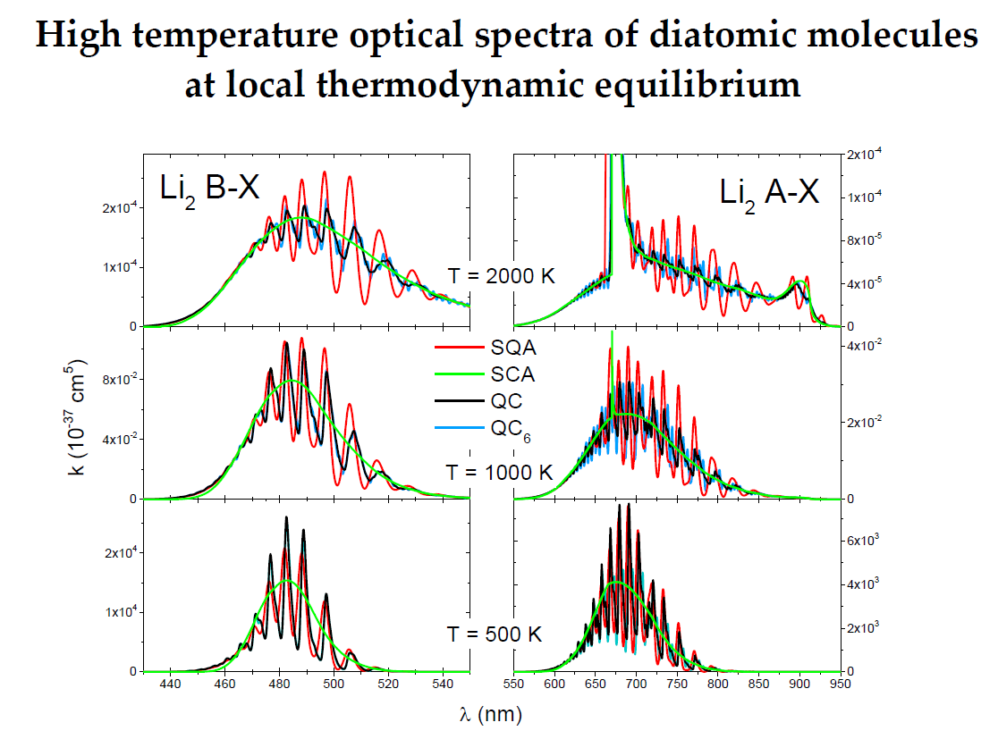
The quasi-static formula generally gives a good description of the absorption coefficient, but it diverges in the difference potential extremes (classical singularities). This divergence can be removed by mapping the phase of the semi-classical canonic integral, into the characteristic form of the elementary catastrophes [8]. In the case where the difference potential has one extreme point $R_e$$\Delta \left(R_e\right)=h{\nu }_e$ and two Condon points, Connor et al. [9] suggested mapping of the phase on the form of the elementary “fold” catastrophe, with a parameter of mapping dependent on the Condon points phase difference. Following these concepts Beuc et al. [10] defined the coherent uniform Airy approximation of the spectral profile, which showed that for frequencies where two real Condon points $R_{1\nu }$ and $R_{2\nu }$$\left(R_{1\nu }\le R_e\le R_{2\nu }\right)$ exist:

$$P(\nu ,T)=\frac{\sqrt{\pi }{\left(2\mu k_{B}T\right)}^{3/2}}{{\hslash }^2}\nu \left\{\begin{array}{l}\left[\frac{R_1^{2}D{(R_1)}^2}{\left|{\Delta }^{\prime }(R_1)\right|}\exp (-\frac{V_{{\mathsf{\Lambda }}^{″}}(R_1)}{k_{B}T})+\frac{R_2^{2}D{(R_2)}^2}{\left|{\Delta }^{\prime }(R_2)\right|}\exp (-\frac{V_{{\mathsf{\Lambda }}^{″}}(R_2)}{k_{B}T})\right]3\sqrt{\pi }(\sqrt{\zeta }L(z)+\frac{1}{\sqrt{\zeta }}H(z))+\\ +2\frac{R_1{}^{2}D(R_1)D(R_2)}{\sqrt{\left|{\Delta }^{\prime }(R_1)\right|\left|{\Delta }^{\prime }(R_2)\right|}}\exp (-\frac{V_{{\mathsf{\Lambda }}^{″}}(R_1)}{k_{B}T})3\sqrt{\pi }(\sqrt{\zeta }L(z)-\frac{1}{\sqrt{\zeta }}H(z))\end{array}\right\}.$$

(18)

Functions $L(z)=\underset{0}{\overset{\infty }{{\displaystyle \int }}}dx\frac{Ai{\left[-zx\right]}^2}{x^2}\exp \left(-1/x^3\right)$ and $H(z)=\underset{0}{\overset{\infty }{{\displaystyle \int }}}dx\frac{Ai\prime {\left[-zx\right]}^2}{x^3}\exp \left(-1/x^3\right)$ are integrals of the square of the Airy function and its first derivative, respectively. Mapping parameter z is defined by the Condon point phase difference $z=z(\nu ,T)={\left(\frac{\mu }{2k_{B}T}\right)}^{\frac{1}{3}}{\left(\frac{3\mathrm{sgn}\left[{\Delta }^{″}(R_e)\right]}{4\hslash }{\displaystyle \underset{R_{1\nu }}{\overset{R_{2v}}{\int }}dR(\Delta (R)-h\nu }\right)}^{\frac{2}{3}}$. Vicharelli et al. [11] derived a similar form of profile using a mapping parameter $z_c=\frac{1}{2}{\left(\frac{\mu }{{\hslash }^2{k}_{B}T}\right)}^{\frac{1}{3}}\frac{{\Delta }^{\prime }{\left(R_c\right)}^2}{{\left|{\Delta }^{″}\left(R_c\right)\right|}^{\frac{4}{3}}}$ locally defined in each Condon point. The same mapping parameter was used in the non-coherent uniform Airy approximation by Szudy and Baylis [12].

After introducing the functions $\mathsf{{\rm N}}(z)=6\sqrt{\pi }L(z)$ and $M(z)=6\sqrt{\pi }\left(H(z)-zL(z)\right)$ the relation in Equation (18) can be reorganized in following form:

$$P(\nu ,T)=\frac{\sqrt{\pi }{\left(2\mu k_{B}T\right)}^{3/2}}{{\hslash }^2}\nu \left\{\begin{array}{l}\left[\frac{R_1^{2}D{(R_1)}^2}{\left|{\Delta }^{\prime }(R_1)\right|}\exp (-\frac{V_{{\mathsf{\Lambda }}^{″}}(R_1)}{k_{B}T})+\frac{R_2^{2}D{(R_2)}^2}{\left|{\Delta }^{\prime }(R_2)\right|}\exp (-\frac{V_{{\mathsf{\Lambda }}^{″}}(R_2)}{k_{B}T})\right]\sqrt{z}\mathsf{{\rm N}}(z)+\\ +\left[\frac{R_1^{2}D{(R_1)}^2}{\left|{\Delta }^{\prime }(R_1)\right|}\exp (-\frac{V_{{\mathsf{\Lambda }}^{″}}(R_1)}{k_{B}T})-2\frac{R_1{}^{2}D(R_1)D(R_2)}{\sqrt{\left|{\Delta }^{\prime }(R_1)\right|\left|{\Delta }^{\prime }(R_2)\right|}}\exp (-\frac{V_{{\mathsf{\Lambda }}^{″}}(R_1)}{k_{B}T})+\frac{R_2^{2}D{(R_2)}^2}{\left|{\Delta }^{\prime }(R_2)\right|}\exp (-\frac{V_{{\mathsf{\Lambda }}^{″}}(R_2)}{k_{B}T})\right]\frac{1}{2\sqrt{z}}\mathsf{{\rm M}}(z)\end{array}\right\}.$$

(19)

If parameter z is larger $z>10$ than $\sqrt{z}\mathsf{{\rm N}}(z)\to 1$ and $\mathsf{{\rm M}}(z)\to 0$ (Figure 1), so it is important to the analyzed profile in the neighborhood of the extreme. The transition dipole moment can be approximated with a linear expansion $D(R)=D(R_e)+D^{\prime }(R_e)(R-R_e)$ and a difference potential with cubic expansion $\Delta (R)=h{\nu }_e+\frac{1}{2}{\Delta }^{″}(R_e){(R-R_e)}^2+\frac{1}{6}{\Delta }^{‴}(R_e){(R-R_e)}^3$. Mapping parameter z in this region has a simple form as described in Reference [13]:

$$z=z_e=z_e(v,T)={\left(\frac{4{\pi }^{2}h\mu }{k_{B}T\left|{\Delta }^{″}(R_e)\right|}\right)}^{\frac{1}{3}}\mathrm{sgn}\left[{\Delta }^{″}(R_e)\right]({\nu }_e-\nu ).$$

(20)

The transitional approximation of the spectral profile in the neighborhood of the extreme gives:

$$P(\nu ,T)=\frac{\sqrt{\pi }{\left(2\mu k_{B}T\right)}^{3/2}}{{\hslash }^2}\nu {\left(\frac{\mu }{8{\hslash }^2{k}_{B}T}\right)}^{\frac{1}{6}}\frac{R_e^2}{{\left|{\Delta }^{″}(R_e)\right|}^{2/3}}{e}^{-\frac{V(R_e)}{k_{B}T}}\left[D{\left(R_e\right)}^2\mathsf{{\rm N}}(z_e)+{\left(\frac{8{\hslash }^2{k}_{B}T}{\mu }\right)}^{\frac{1}{3}}\frac{{\left[D^{\prime }(R_e)-D\left(R_e\right)\frac{{\Delta }^{‴}(R_e)}{6{\Delta }^{″}(R_e)}\right]}^2}{{\left|{\Delta }^{″}(R_e)\right|}^{\frac{2}{3}}}M(z_e)\right].$$

(21)

First part in Equation (21) is the contribution of the Condon points pair, and it can be used as an analytical continuation in the classically forbidden region, where $z_e\le 0$. The second part contains the interference contribution of the neighboring Condon points and depends on two parameters: $D^{\prime }(R_e)$ and ${\Delta }^{‴}(R_e)/{\Delta }^{″}(R_e)$. The first parameter is important in the case of a strongly varying transition dipole moment as pointed out in Reference [9]. The second parameter, defined by the anharmonicity of the difference potential in the neighborhood of the extreme, was extensively discussed in Reference [14]. Even in the case when the dipole moment at the extreme goes through zero [15], there is a non-vanishing contribution to the spectral profile given by the second part in Equation (21). Behavior of the functions $\sqrt{z}\mathsf{{\rm N}}(z)$, $\mathsf{{\rm N}}(z)$, and M(z) suggest that it is most important to know the function $z(v,T)$ in the neighborhood of the extreme, so we approximated this function in a whole range of frequencies with $z(\nu ,T)=z_e(v,T)$. Using the same reasoning, we approximated the last part in the parenthesis of Equation (19) by the corresponding contribution of the transitional approximation in Equation (21). The spectral profile can be written as:

$$P(\nu ,T)=\frac{\sqrt{\pi }{\left(2\mu k_{B}T\right)}^{3/2}}{{\hslash }^2}\nu \left\{\begin{array}{l}{\displaystyle \sum _{i=1}^2\frac{R_i^{2}D{(R_i)}^2}{\left|{\Delta }^{\prime }(R_i)\right|}\exp (-\frac{V_{{\mathsf{\Lambda }}^{″}}(R_i)}{k_{B}T})\sqrt{z_e}\mathsf{{\rm N}}(z_i)\mathsf{\Theta }\left(z_e\right)}+{\left(\frac{\mu }{8{\hslash }^2{k}_{B}T}\right)}^{\frac{1}{6}}\frac{R_e^{2}D{\left(R_e\right)}^2}{{\left|{\Delta }^{″}(R_e)\right|}^{2/3}}{e}^{-\frac{V(R_e)}{k_{B}T}}\mathsf{{\rm N}}(z_e)\mathsf{\Theta }\left(-z_e\right)\\ +{\left(\frac{8{\hslash }^2{k}_{B}T}{\mu }\right)}^{\frac{1}{6}}\frac{R_e^2{\left[D^{\prime }(R_e)-D\left(R_e\right)\frac{{\Delta }^{‴}(R_e)}{6{\Delta }^{″}(R_e)}\right]}^2}{{\left|{\Delta }^{″}(R_e)\right|}^{4/3}}{e}^{-\frac{V(R_e)}{k_{B}T}}M(z_e)\end{array}\right\}.$$

(22)

The first part in Equation (22) describes the contribution of the Condon points in the classically allowed region, the second part contribution of the Condon points pair in the classically forbidden region, and the third part, its interference in the whole region of frequencies.

If the difference potential has $n_e$ extremes with the position and frequency $\Delta \left(R_{ei}\right)=h{\nu }_{ei}$, $R_{e1}<R_{e2}<...$ then there are $n_e+1$ Condon points $R_1\le R_{e1}\le R_2\le R_{e2}\le R_3\le ...$. In the neighborhood of i-th extreme, a parameter $z_{ei}={\left(\frac{4{\pi }^{2}h\mu }{k_{B}T\left|{\Delta }^{″}(R_{ei})\right|}\right)}^{\frac{1}{3}}\mathrm{sgn}\left[{\Delta }^{″}(R_{ei})\right]({\nu }_{ei}-\nu )$ can be defined and the contribution of the Condon points R_i and R_i+1 to the spectral profile is given by the relation in Equation (22). If extremes are well separated, by analogy to Equation (22), a generalized uniform Airy approximation can be written as:

$$P(\nu ,T)=\frac{\sqrt{\pi }{\left(2\mu k_{B}T\right)}^{3/2}}{{\hslash }^2}\nu \left\{\begin{array}{l}{\displaystyle \sum _{i=1}^{n_e+1}\frac{R_i^{2}D{(R_i)}^2}{\left|{\Delta }^{\prime }(R_i)\right|}\exp (-\frac{V_{{\mathsf{\Lambda }}^{″}}(R_i)}{k_{B}T})\sqrt{z_i}\mathsf{{\rm N}}(z_i)\mathsf{\Theta }\left(z_i\right)}+\\ +{\left(\frac{\mu }{8{\hslash }^2{k}_{B}T}\right)}^{\frac{1}{6}}{\displaystyle \sum _{i=1}^{n_e}\frac{R_{ei}^{2}D{\left(R_{ei}\right)}^2}{{\left|{\Delta }^{″}(R_{ei})\right|}^{2/3}}{e}^{-\frac{V(R_e)}{k_{B}T}}\mathsf{{\rm N}}(z_{ei})\mathsf{\Theta }\left(-z_{ei}\right)+}\\ +{\left(\frac{8{\hslash }^2{k}_{B}T}{\mu }\right)}^{\frac{1}{6}}{\displaystyle \sum _{i=1}^{n_e}\frac{R_{ei}^2{\left[D^{\prime }(R_{ei})-D\left(R_{ei}\right)\frac{{\Delta }^{‴}(R_{ei})}{6{\Delta }^{″}(R_{ei})}\right]}^2}{{\left|{\Delta }^{″}(R_{ei})\right|}^{4/3}}{e}^{-\frac{V(R_e)}{k_{B}T}}M(z_{ei})}\end{array}\right\}.$$

(23)

If two extremes exist, a problem strictly belongs to the class of higher elementary “cusp” catastrophes. The uniform Airy approximation can be applied with the following choice of functions z. For the first Condon point ($R_1\le R_{e1}$), the choice is $z_1=z_{e1}$, and for the last one ($R_3\ge R_{e2}$) $z_3=z_{e2}$. For the middle Condon point ($R_{e1}\le R_2\le R_{e2}$), in the neighborhood of the first extreme, the correct choice is $z_2=z_{e1}$, and the near second extreme $z_2=z_{e2}$, and we suggest that in the whole real range of the Condon point $R_2$, the approximation $z_2=\min \left(z_{e1},z_{e2}\right)$. Similarly, in the case of three extremes (swallowtail catastrophe), we suggest $z_1=z_{e1}$,$z_2=\min \left(z_{e1},z_{e2}\right)$, $z_3=\min \left(z_{e2},z_{e3}\right)$$z_4=z_{e3}$. For a larger number of extremes, what is not a common physical case, the use of the relation in Equation (22) may be very questionable.

As in the case of a quasi-static formula one can the estimate contributions of bound–bound, bound–free, and transition in Equations (22) and (23) by a simple substitution of the statistical weight factor $n_{xx}(T,R)R^2\exp (-\frac{V_{{\mathsf{\Lambda }}^{″}}(R)}{k_{B}T})$ instead of $R^2\exp (-\frac{V_{{\mathsf{\Lambda }}^{″}}(R)}{k_{B}T})$ for each Condon and extreme point.

Numerical values of the function L(z) are given in Reference [12], and we gave a table with the numerical values of the functions N(z) and M(z) as Supplementary data in Table S1.

3.2. Quantum Calculation on the Fourier Grid

To calculate the energies and wavefunctions of the ro-vibrational states, the FGH method (Fourier grid Hamiltonian) was used as a special case of Discrete Variable Representation, where functions were represented on a finite number of grid points R_i (i = 1…N) [16,17]. Grid of uniformly spaced points was used ${\Delta }_R=R_{i+1}-R_i$ and the energies and wave functions could be determined by diagonalization of N × N Hamiltonian matrix:

$$H_{\mathsf{\Lambda }J}=\left\{\begin{array}{cc}\frac{{\hslash }^2}{2\mu \Delta R^2}\left(\frac{{\pi }^2}{3}-\frac{1}{2i^2}\right)+V_{\mathsf{\Lambda }}(R_i)+\frac{{\hslash }^2}{2\mu }\frac{J(J+1)-{\mathsf{\Lambda }}^2}{R_i{}^2}& i=j\\ {\left(-1\right)}^{i-j}\frac{{\hslash }^2}{2\mu \Delta R^2}\frac{8ij}{{\left(i^2-j^2\right)}^2}& i\ne j\end{array}\right\}.$$

(24)

Solving the Schrödinger equation in the matrix form $H_{\mathsf{\Lambda }J}{\mathsf{\Phi }}_{\mathsf{\Lambda }J}={\mathsf{{\rm E}}}_{\mathsf{\Lambda }J}{\mathsf{\Phi }}_{\mathsf{\Lambda }J}$, one obtains a column matrix ${\mathsf{{\rm E}}}_{\mathsf{\Lambda }J}$ containing N energies $E_{vJ\mathsf{\Lambda }}$ and an N × N matrix ${\mathsf{\Phi }}_{\mathsf{\Lambda }J}$, where the columns contain values of wave functions at grid points ${\phi }_{vJ\mathsf{\Lambda }}(R_i)$. All transition matrix elements of the electronic transition dipole moment D(R) can be calculated by a matrix multiplication $\langle {\phi }_{{\mathrm{v}}^{″},J^{″},{\mathsf{\Lambda }}^{″}}\left|D(R)\right|{\phi }_{{\mathrm{v}}^{\prime },J^{\prime },{\mathsf{\Lambda }}^{\prime }}\rangle ={\left[{\mathsf{\Phi }}_{{\mathsf{\Lambda }}^{″}{J}^{″}}{D}_G{\mathsf{\Phi }}_{{\mathsf{\Lambda }}^{\prime }{J}^{\prime }}^T\right]}_{v^{″}{v}^{\prime }}$, where $D_G$ is the diagonal matrix with diagonal containing values of transition dipole moments at grid points $D(R_i)$. Transition frequencies can be also calculated using a simple matrix operation ${\nu }_{tr}=\left(E_{v^{\prime }{J}^{\prime }{\mathsf{\Lambda }}^{\prime }}-E_{v^{″}{J}^{″}{\mathsf{\Lambda }}^{″}}\right)/h={\left[{(U\cdot E_{J^{\prime }{\mathsf{\Lambda }}^{\prime }})}^T-U\cdot E_{J^{″}{\mathsf{\Lambda }}^{″}}\right]}_{v^{\prime }{v}^{″}}/h$, where U is the N × N matrix with all elements equal to 1.

The method yields only a discrete set of continuum energies, but in the range spanned by the grid, the corresponding unity-normalized wave functions represent the states of a continuum. The continuum of free states is represented by a discrete set of unity-normalized wave functions having a node at the outer grid boundary $R_N=N{\Delta }_R$. Space between the neighboring grid point $\Delta R$ is done using the relation ${\Delta }_R=\frac{2\pi \hslash }{n_B\sqrt{2\mu E_{\max }}}$, where n_B is the number of grid points per de Broglie wavelength (we obtained satisfactory results choosing n_B > 2) at a maximal expected kinetic energy $E_{\max }$. Let $E_T=\frac{3}{2}{k}_B{T}_M$ be the energy at the maximal temperature which occured in the calculation. Choosing $E_{\max }=5E_{T_M}$ and $n_B=\frac{2\pi }{\sqrt{5}}=2.8$ one obtains ${\Delta }_R=\frac{\hslash }{\sqrt{2\mu E_T}}$. The end grid point R_N was chosen to allow the energy $V_{\mathsf{\Lambda }}(R_N)$ to get closer to the molecular dissociation energy. Approximating the free state energies in FGH with energies in the infinite square well potential of length $R_N$ one obtains $E_n=\frac{{\pi }^2{\hslash }^2}{2\mu R_N^2}{n}^2$ and $E_N={\pi }^2{E}_T\approx 10E_T$. Given the temperature T, a population of the molecular states with energy lower than $E_N$ can be approximated (using the analogy with the relation in Equation (14)) with $n\left(T\right)=\frac{2}{\sqrt{\pi }}\gamma \left(\frac{3}{2},\frac{E_N)}{k_{B}T}\right)$. For the maximal expected temperature $n\left(T_M\right)=\frac{2}{\sqrt{\pi }}\gamma \left(\frac{3}{2},15\right)=0.999999$, we concluded that the molecular states on the grid completely represented all the free states for temperatures $T\le T_M$. It can be written that $E_n=10E_T{\left(\frac{n}{N}\right)}^2$, and concluded that the increasing number of grid points increased the number of free states, but the highest energy $E_N$ remained unchanged. It is important to keep in mind that the evaluation of the Hamiltonian matrix eigenvalues consumes time in a manner proportional with $N^{\frac{5}{2}}$, so increasing the number of grid points N can drastically increase the computational time.

3.2.1. Full Quantum Calculation

Solving the radial Schrödinger equation on the grid, one obtains a set of discrete states effectively describing a confined molecule, “a molecule in a box,” and the entire spectrum is of the bound–bound type [18]:

$$P(\nu ,T)=\nu {\displaystyle \sum _{J^{″}={\mathsf{\Lambda }}^{″}}^{J_M}{\omega }_{J``}(2J^{″}+1){\displaystyle \sum _{v``=0,v^{\prime }=0}^{N,N}{e}^{-\frac{E_{v``J``\mathsf{\Lambda }``}}{k_{B}T}}{\displaystyle \sum _{\Delta J=-1}^1\frac{S_{J``\mathsf{\Lambda }``}^{\left(J``-\Delta J\right)\mathsf{\Lambda }`}}{(2J^{″}+1)}{\left|\langle {\phi }_{v``J``\mathsf{\Lambda }``}\left|D(R)\right|{\phi }_{v`\left(J``-\Delta J\right)\mathsf{\Lambda }`}\rangle \right|}^2}}}g(\nu -{\nu }_{tr\Delta J}).$$

(25)

The maximal $J_M$ value in the sum is determined as the $J^{″}$-value for which the repulsive rotational term at the end grid point $R_N$ is equal to the energy $E_T$, which follows $J_M\approx \frac{R_N}{\hslash }\sqrt{2\mu E_T}$ and $J_M=N$.

The last sum in the relation in Equation (25) contains contributions to the P, Q, R branches of the spectra for $\Delta J=-1,0,1$, respectively. For each $J^{″}$ value in Equation (25), there are N energies and wave functions in the lower ${\mathsf{\Lambda }}^{″}$ and upper ${\mathsf{\Lambda }}^{\prime }$ electronic states, and consequently, $N^2$ transitions between the ro-vibrational states of the lower and upper electronic state. Each transition “i” is defined by numbers $({v^{″}}_i,{v^{\prime }}_i,{J^{″}}_i,\Delta J_i)$ and the number of transitions is $M=3N^3$, where factor 3 is because of the P, Q, R branching.

Using the first order perturbation approach, one gets $|{\phi }_{v^{\prime }\left(J^{″}+\Delta J\right){\mathsf{\Lambda }}^{\prime }}\rangle \approx |{\phi }_{v^{\prime }{J}^{″}{\mathsf{\Lambda }}^{\prime }}\rangle$, $E_{v^{\prime }\left(J^{″}+{\Delta }_J\right){\mathsf{\Lambda }}^{\prime }}\approx E_{v^{\prime }{J}^{″}{\mathsf{\Lambda }}^{\prime }}+hc{B}_{v^{\prime }{J}^{″}{\mathsf{\Lambda }}^{\prime }}(2J^{″}+\Delta J+1)\Delta J$ where $B_{v^{\prime }{J}^{″}{\mathsf{\Lambda }}^{\prime }}=\frac{{\hslash }^2}{2\mu hc}\langle {\phi }_{v^{\prime }{J}^{″}{\mathsf{\Lambda }}^{\prime }}\left|\frac{1}{R^2}\right|{\phi }_{v^{\prime }{J}^{″}{\mathsf{\Lambda }}^{\prime }}\rangle$. We can write that:

$${\displaystyle \sum _{\Delta J=-1}^1\frac{S_{J``\mathsf{\Lambda }``}^{\left(J``-\Delta J\right)\mathsf{\Lambda }`}}{(2J^{″}+1)}{\left|\langle {\phi }_{v``J``\mathsf{\Lambda }``}\left|D(R)\right|{\phi }_{v`\left(J``-\Delta J\right)\mathsf{\Lambda }`}\rangle \right|}^2}g(\nu -{\nu }_{tr\Delta })\approx {\left|\langle {\phi }_{v``J``\mathsf{\Lambda }``}\left|D(R)\right|{\phi }_{v`J``\mathsf{\Lambda }`}\rangle \right|}^2{\displaystyle \sum _{\Delta J=-1}^1\frac{S_{J``\mathsf{\Lambda }``}^{\left(J``-\Delta J\right)\mathsf{\Lambda }`}}{(2J^{″}+1)}}g(\nu -{\nu }_{tr\Delta }),$$

(26)

where transition frequency is ${\nu }_{tr{\Delta }_J}={\nu }_{tr0}+c{B}_{v^{\prime }{J}^{″}{\mathsf{\Lambda }}^{\prime }}(2J^{″}+\Delta J+1)\Delta J$. If the splitting between the branches is not resolved by the spectrometer, the Q-branch or $\Delta J=0$ approximation can be applied:

$${\displaystyle \sum _{\Delta J=-1}^1\frac{S_{J``\mathsf{\Lambda }``}^{\left(J``-\Delta J\right)\mathsf{\Lambda }`}}{(2J^{″}+1)}}g(\nu -{\nu }_{tr\Delta })\approx g(\nu -{\nu }_{tr\Delta J=0})$$

(27)

In the case of a low spectral resolution, using the Q-branch approximation, summation over $J^{″}$ can be replaced with the summation over the $k_M$ intervals of $J^{″}$ values, where the number of intervals $k_M$ is the nearest integer of $\frac{N}{n}$ . Using the relation in Equation (A2) it follows that:

$$P(\nu ,T,n)={\overline{\omega }}_{J``}\nu {\displaystyle \sum _{v^{″}=0,v^{\prime }=0}^{N,N}{\displaystyle \sum _{k=0}^{k_M}n\left[2(kn+\mathsf{\Lambda })+n\right]}{e}^{-\frac{E_{v``J_k\mathsf{\Lambda }``}}{k_{B}T}}{\left|\langle {\phi }_{v``J_k\mathsf{\Lambda }``}\left|D(R)\right|{\phi }_{v`J_k\mathsf{\Lambda }`}\rangle \right|}^2}\overline{g}(\nu -{\nu }_{t{r}_k}),$$

(28)

where ${\overline{\omega }}_{J``}$ is the averaged factor ${\omega }_{J``}$ equal to 1 for heteronuclear and 1/2 for homonuclear molecules and $J_k(J_k+1)=\left(kn+\mathsf{\Lambda }\right)(kn+\mathsf{\Lambda }+n)+\frac{1}{2}(n^2-1)$. The number of transitions $({v^{″}}_i,{v^{\prime }}_i,k)$ is $M=k_M{N}^2$.

Furthermore, the abbreviation QC will be used to represent the reduced absorption coefficient obtained with the equation $P(\nu ,T,1)$ and QCn with the equation $P(\nu ,T,n)$.

3.2.2. Vibration Band Approximation (VBA)

The relation in Equation (25) can be written as:

$$P(\nu ,T)=\nu {\displaystyle \sum _{v^{″}=0,v^{\prime }=0}^{N,N}\exp \left(-\frac{E_{v^{″}{\mathsf{\Lambda }}^{″}{\mathsf{\Lambda }}^{″}}}{k_{B}T}\right)}{\displaystyle \sum _{J^{″}={\mathsf{\Lambda }}^{″}}^N{\omega }_{J^{″}}(2J^{″}+1)\exp \left(-\frac{E_{v^{″}{J}^{″}{\mathsf{\Lambda }}^{″}}-E_{v^{″}{\mathsf{\Lambda }}^{″}{\mathsf{\Lambda }}^{″}}}{k_{B}T}\right)}{\displaystyle \sum _{\Delta J=-1}^1\frac{S_{J^{″}{\mathsf{\Lambda }}^{″}}^{\left(J^{″}-\Delta J\right){\mathsf{\Lambda }}^{\prime }}}{(2J^{″}+1)}{\left|\langle {\phi }_{v^{″}{J}^{″}{\mathsf{\Lambda }}^{″}}\left|D(R)\right|{\phi }_{v^{\prime }\left(J^{″}-\Delta J\right){\mathsf{\Lambda }}^{\prime }}\rangle \right|}^2}g(\nu -{\nu }_{tr\Delta }).$$

(29)

An interesting task was imposed to calculate the vibrational transition profile (sum over $J^{″}$ and $\Delta J$). Using the first order perturbation approach one obtains:

$|{\phi }_{vJ\mathsf{\Lambda }}\rangle \approx |{\phi }_{v0\mathsf{\Lambda }}\rangle$, $\langle {\phi }_{v^{″}{J}^{″}{\mathsf{\Lambda }}^{″}}\left|D(R)\right|{\phi }_{v^{\prime }{J}^{\prime }{\mathsf{\Lambda }}^{\prime }}\rangle \approx \langle {\phi }_{v^{″}{\mathsf{\Lambda }}^{″}{\mathsf{\Lambda }}^{″}}\left|D(R)\right|{\phi }_{v^{\prime }{\mathsf{\Lambda }}^{″}{\mathsf{\Lambda }}^{\prime }}\rangle$, $E_{vJ\mathsf{\Lambda }}\approx E_{v0\mathsf{\Lambda }}+hc{B}_{v\mathsf{\Lambda }}J(J+1)$, transition frequency ${\upsilon }_{tr}\approx E_{v^{\prime },v^{″}}/h+c{B}_{v^{\prime },v^{″}}{J}^{″}(J^{″}+1)-c{B}_{v^{\prime }{\mathsf{\Lambda }}^{\prime }}\left(2J^{″}-\Delta J\right)\Delta J$, where $B_{v\mathsf{\Lambda }}=\frac{{\hslash }^2}{2\mu hc}\langle {\phi }_{v{\mathsf{\Lambda }}^{″}\mathsf{\Lambda }}\left|\frac{1}{R^2}\right|{\phi }_{v{\mathsf{\Lambda }}^{″}\mathsf{\Lambda }}\rangle$, $E_{v^{\prime }{v}^{″}}=E_{v^{\prime }0{\mathsf{\Lambda }}^{\prime }}-E_{v^{\prime }0{\mathsf{\Lambda }}^{\prime }}$, $B_{v^{\prime }{v}^{″}}=B_{v^{\prime }{\mathsf{\Lambda }}^{\prime }}-B_{v^{″}{\mathsf{\Lambda }}^{″}}$.

Applying this approximation to the bound vibrational states only we write:

$$P(\nu ,T)=\nu {\displaystyle \sum _{v^{″}=0,v^{\prime }=0}^{V^{″},V^{\prime }}\exp \left(-\frac{E_{v^{″}{\mathsf{\Lambda }}^{″}{\mathsf{\Lambda }}^{″}}}{k_{B}T}\right)}{\left|\langle {\phi }_{v^{″}{\mathsf{\Lambda }}^{″}{\mathsf{\Lambda }}^{″}}\left|D(R)\right|{\phi }_{v^{\prime }{\mathsf{\Lambda }}^{″}{\mathsf{\Lambda }}^{\prime }}\rangle \right|}^2{\displaystyle \sum _{J^{″}={\mathsf{\Lambda }}^{″}}^N{\omega }_{J``}(2J^{″}+1)\exp \left(-\frac{hc{B}_{v^{″}}{J}^{″}(J^{″}+1)}{k_{B}T}\right)}{\displaystyle \sum _{\Delta J=-1}^1\frac{S_{J``\mathsf{\Lambda }``}^{\left(J``-\Delta J\right)\mathsf{\Lambda }`}}{(2J^{″}+1)}}g(\nu -{\nu }_{tr\Delta }).$$

(30)

$V^{″}$ and $V^{\prime }$ are the vibrational wave numbers of the highest bound vibrational state in the lower electronic state ${\mathsf{\Lambda }}^{″}$ and upper state ${\mathsf{\Lambda }}^{\prime }$, respectively. The number of transitions $({v^{″}}_i,{v^{\prime }}_i,{J^{″}}_i,\Delta J_i)$ is $M=3N{V}^{″}{V}^{\prime }$. In the Q-branch approximation the relation in Equation (30) has a simpler form:

$$P(\nu ,T)=\nu {\displaystyle \sum _{v^{″}=0,v^{\prime }=0}^{V^{″},V^{\prime }}\exp \left(-\frac{E_{v^{″}{\mathsf{\Lambda }}^{″}{\mathsf{\Lambda }}^{″}}}{k_{B}T}\right)}{\left|\langle {\phi }_{v^{″}{\mathsf{\Lambda }}^{″}{\mathsf{\Lambda }}^{″}}\left|D(R)\right|{\phi }_{v^{\prime }{\mathsf{\Lambda }}^{″}{\mathsf{\Lambda }}^{\prime }}\rangle \right|}^2{\displaystyle \sum _{J^{″}={\mathsf{\Lambda }}^{″}}^N{\omega }_{J^{″}}(2J^{″}+1)\exp \left(-\frac{hc{B}_{v^{″}}{J}^{″}(J^{″}+1)}{k_{B}T}\right)}g(\nu -{\nu }_{tr0}).$$

(31)

The number of transitions $({v^{″}}_i,{v^{\prime }}_i,{J^{″}}_i)$ is $M=J_M{V}^{″}{V}^{\prime }$. The reduced absorption coefficient obtained using Equation (31) will be named VBA.

Neglecting the discreetness of the rotational structure, the sum over $J^{″}$ can be calculated analytically:

$$P(\nu ,T)={\omega }_J\frac{\nu }{c}{\displaystyle \sum _{v^{″}=0,v^{\prime }=0}^{V``,V`}\frac{{\left|\langle {\phi }_{v^{″}{\mathsf{\Lambda }}^{″}{\mathsf{\Lambda }}^{″}}\left|D(R)\right|{\phi }_{v^{\prime }{\mathsf{\Lambda }}^{″}{\mathsf{\Lambda }}^{\prime }}\rangle \right|}^2}{\left|B_{v^{\prime }{v}^{″}}\right|}}\exp \left(-\frac{E_{v^{″}{\mathsf{\Lambda }}^{″}{\mathsf{\Lambda }}^{″}}}{k_{B}T}-\frac{B_{v^{″}}h(\nu -{\nu }_{v^{\prime }{v}^{″}})}{B_{v^{\prime }{v}^{″}}{k}_{B}T}\right)\mathsf{\Theta }\left(\frac{\nu -{\nu }_{v^{\prime }{v}^{″}}}{B_{v^{\prime }{v}^{″}}}\right),$$

(32)

where ${\upsilon }_{v^{\prime }{v}^{″}}=E_{v^{\prime },v^{″}}/h$. In the literature, this approach is called the Vibration band continuum approximation (VBCA) [1,19].

The energy $E_{v^{″}{\mathsf{\Lambda }}^{″}{\mathsf{\Lambda }}^{″}}$ in Equation (29) has the meaning of the vibrational energy and $E_{v^{″}{J}^{″}{\mathsf{\Lambda }}^{″}}-E_{v^{″}{\mathsf{\Lambda }}^{″}{\mathsf{\Lambda }}^{″}}$ is the rotational energy of the ro-vibrational state ($v^{″}{J}^{″}{\mathsf{\Lambda }}^{″}$). Assuming a non-LTE case depending on two temperatures (vibrational $T_v$ and rotational $T_R$), the shape of the absorption spectra can be written as follows:

$$P(\nu ,T_V,T_R)=\nu {\displaystyle \sum _{v^{″}=0,v^{\prime }=0}^{N,N}\exp \left(-\frac{E_{v^{″}{\mathsf{\Lambda }}^{″}{\mathsf{\Lambda }}^{″}}}{k_B{T}_V}\right)}{\displaystyle \sum _{J^{″}={\mathsf{\Lambda }}^{″}}^N{\omega }_{J^{″}}(2J^{″}+1)\exp \left(-\frac{E_{v^{″}{J}^{″}{\mathsf{\Lambda }}^{″}}-E_{v^{″}{\mathsf{\Lambda }}^{″}{\mathsf{\Lambda }}^{″}}}{k_B{T}_R}\right)}{\displaystyle \sum _{\Delta J=-1}^1\frac{S_{J^{″}{\mathsf{\Lambda }}^{″}}^{\left(J^{″}-\Delta J\right){\mathsf{\Lambda }}^{\prime }}}{(2J^{″}+1)}{\left|\langle {\phi }_{v^{″}{J}^{″}{\mathsf{\Lambda }}^{″}}\left|D(R)\right|{\phi }_{v^{\prime }\left(J^{″}-\Delta J\right){\mathsf{\Lambda }}^{\prime }}\rangle \right|}^2}g(\nu -{\nu }_{tr\Delta })$$

3.2.3. Semi-Quantum Approximation (SQA)

Beuc et al. [18] calculated the vibrational transition profile in the relation in Equation (29) using the classical Franck-Condon principle and the standard semi-classical approach:

$${\displaystyle \sum _{J^{″}={\mathsf{\Lambda }}^{″}}^N{\omega }_{J``}(2J^{″}+1)\exp \left(-\frac{hc{B}_{v^{″}}{J}^{″}(J^{″}+1)}{k_{B}T}\right)}{\displaystyle \sum _{\Delta J=-1}^1\frac{S_{J``\mathsf{\Lambda }``}^{\left(J``-\Delta J\right)\mathsf{\Lambda }`}}{(2J^{″}+1)}}g(\nu -{\nu }_{tr\Delta })\approx {\overline{\omega }}_J\frac{2\mu k_{B}T}{{\hslash }^2}{\left|\langle {\phi }_{v^{″}{\mathsf{\Lambda }}^{″}{\mathsf{\Lambda }}^{″}}\left|RD(R)\right|{\phi }_{v^{\prime }{\mathsf{\Lambda }}^{″}{\mathsf{\Lambda }}^{\prime }}\rangle \right|}^2\delta (\nu -{\nu }_{tr})$$

(33)

Using this approximation, the spectral profile acquires the form:

$$P(\nu ,T)\approx \nu {\overline{\omega }}_J\frac{2\mu k_{B}T}{{\hslash }^2}{\displaystyle \sum _{{\mathrm{v}}^{″},{\mathsf{\nu }}^{\prime }}^{N,N}\exp (-\frac{E_{v^{″}{\mathsf{\Lambda }}^{″}{\mathsf{\Lambda }}^{″}}}{k_{B}T}){\left|\langle {\phi }_{v^{″}{\mathsf{\Lambda }}^{″}{\mathsf{\Lambda }}^{″}}\left|RD(R)\right|{\phi }_{v^{\prime }{\mathsf{\Lambda }}^{″}{\mathsf{\Lambda }}^{\prime }}\rangle \right|}^{2}g(\nu -{\nu }_{tr})}.$$

(34)

This expression was formally obtained by a completely semi-classical procedure, but it was “dressed” in quantum-like form, so the authors called it the semi-quantum approximation (SQA). In order to calculate the relation in Equation (33), only one diagonalization of the Hamiltonian matrix for the upper and lower electronic state, respectively, is required. The number of transitions $({v^{″}}_i,{v^{\prime }}_i)$ is $M=N^2$.

3.2.4. Numerical Calculation of the Spectral Profile

The numerical calculation of the spectral profiles given by Equations (25, 28, 30, 31, 34) comprises two steps. The first one is to calculate all elements of the $3\times M$ matrix $P_{tr}$ in which the i-th raw contains the transition frequency ${\nu }_{tr}^{(i)}$, energy of initial ro-vibrational state $E^{(i)}$, and amplitude $A^{\left(i\right)}$ (

Table 1. Transition amplitude.

Amplitude ${\mathit{A}}^{\left(\mathit{i}\right)}$	Equation
${\omega }_{J_i``}{S}_{J_i``\mathsf{\Lambda }``}^{\left(J_i``-\Delta J_i\right)\mathsf{\Lambda }`}{\left|\langle {\phi }_{v_i``J_i``\mathsf{\Lambda }``}\left|D(R)\right|{\phi }_{v_i`\left(J_i``-\Delta J_i\right)\mathsf{\Lambda }`}\rangle \right|}^2$	(25)
${\overline{\omega }}_{J}n\left[2(k_{i}n+\mathsf{\Lambda })+n\right]{\left|\langle {\phi }_{v_i``J_{k_i}\mathsf{\Lambda }``}\left|D(R)\right|{\phi }_{v_i`J_{k_i}\mathsf{\Lambda }`}\rangle \right|}^2$	(28)
${\omega }_{J_i``}{S}_{J_i``\mathsf{\Lambda }``}^{\left(J_i``-\Delta J_i\right)\mathsf{\Lambda }`}{\left|\langle {\phi }_{v_i``0\mathsf{\Lambda }``}\left|D(R)\right|{\phi }_{v_i`0\mathsf{\Lambda }`}\rangle \right|}^2$	(30)
${\omega }_{J_i``}(2J_i{}^{\prime \prime }+1){\left|\langle {\phi }_{v_i``0\mathsf{\Lambda }``}\left|D(R)\right|{\phi }_{v_i`0\mathsf{\Lambda }`}\rangle \right|}^2$	(31)
${\overline{\omega }}_J\frac{2\mu k_{B}T}{{\hslash }^2}{\left|\langle {\phi }_{\mathrm{v}″,0,\mathsf{\Lambda }″}\left|RD(R)\right|{\phi }_{\mathrm{v}\prime ,0,\mathsf{\Lambda }\prime }\rangle \right|}^2$	(34)

).

The second step is to calculate the spectra using elements of the matrix $P_{tr}$. Equations (24, 28, 30, 31, 34) can be transformed into a single sum:

$$P(\nu ,T)=\nu {\displaystyle \sum _{i=0}^{M}Exp\left(-\frac{E^{(i)}}{k_{B}T}\right)A^{(i)}}g(\nu -{\nu }_{tr}^{(i)}).$$

(35)

In the wavelength domain [20], the spectral profile is given by the relation:

$$P(\lambda ,T)=\frac{\lambda }{\Delta \lambda }{\displaystyle \sum _{}^{\Delta \lambda }Exp\left(-\frac{E^{(i)}}{k_{B}T}\right)A^{(i)}}.$$

(36)

The line profile $g(\lambda -{\lambda }_{tr}^{(i)})$ is approximated with a Heaviside pi (or box car) function $g(\lambda -{\lambda }_{tr}^{(i)})\to \frac{1}{\Delta \lambda }{h}_{\pi }(\frac{\lambda -{\lambda }_{tr}^{(i)}}{\Delta \lambda })$, where the optical transition wavelength is ${\lambda }_{tr}^{(i)}=c/{\nu }_{tr}^{(i)}$ and $\Delta \lambda$ is equal to or larger than the line profile half width and smaller than the instrumental half width. In the evaluation of the relation in Equation (36), the time consumption is proportional to the number of ro-vibrational transitions M. To make the evaluation time efficient we used the matrix $\overline{P}\subseteq P_{tr}$, elements of which satisfied the condition ${\lambda }_{tr}^{(i)}\in ({\lambda }_{\min },{\lambda }_{\max })$, where the interval $({\lambda }_{\min },{\lambda }_{\max })$ was a spectral region of our interest.

4. Results

To explain the characteristics of the theoretical approaches described in the previous section, we compared them on the examples of absorption spectra of a heteronuclear $Li-He$ molecule and homonuclear $L{i}_2$ and $C{s}_2$ molecules. Owing to the very small spin-orbit splitting in the Li atom (for Li$2P_{1/2,3/2}$, ${\Delta }_{fs}=0.335{\mathrm{cm}}^{-1}$), we used for the $Li-He$ and $L{i}_2$ molecules, relevant potential curves and transition dipole moments calculated on a Hund’s case (a) basis, but for the $C{s}_2$ molecule with strong spin-orbit splitting (for $6P_{1/2,3/2}$${\Delta }_{fs}=554.039{\mathrm{cm}}^{-1}$) we used the calculation on a Hund’s case (c) basis. ${}^{7}Li-{}^4\mathit{He}$ and ${}^{7}L{i}_2$ molecules had small reduced masses $\mu =2.54862$ and $\mu =3.508$, respectively, in comparison with the reduced mass $\mu =66.453$ of the ${}^{137}C{s}_2$ molecule. what is important for dynamic in molecules and influences their spectra.

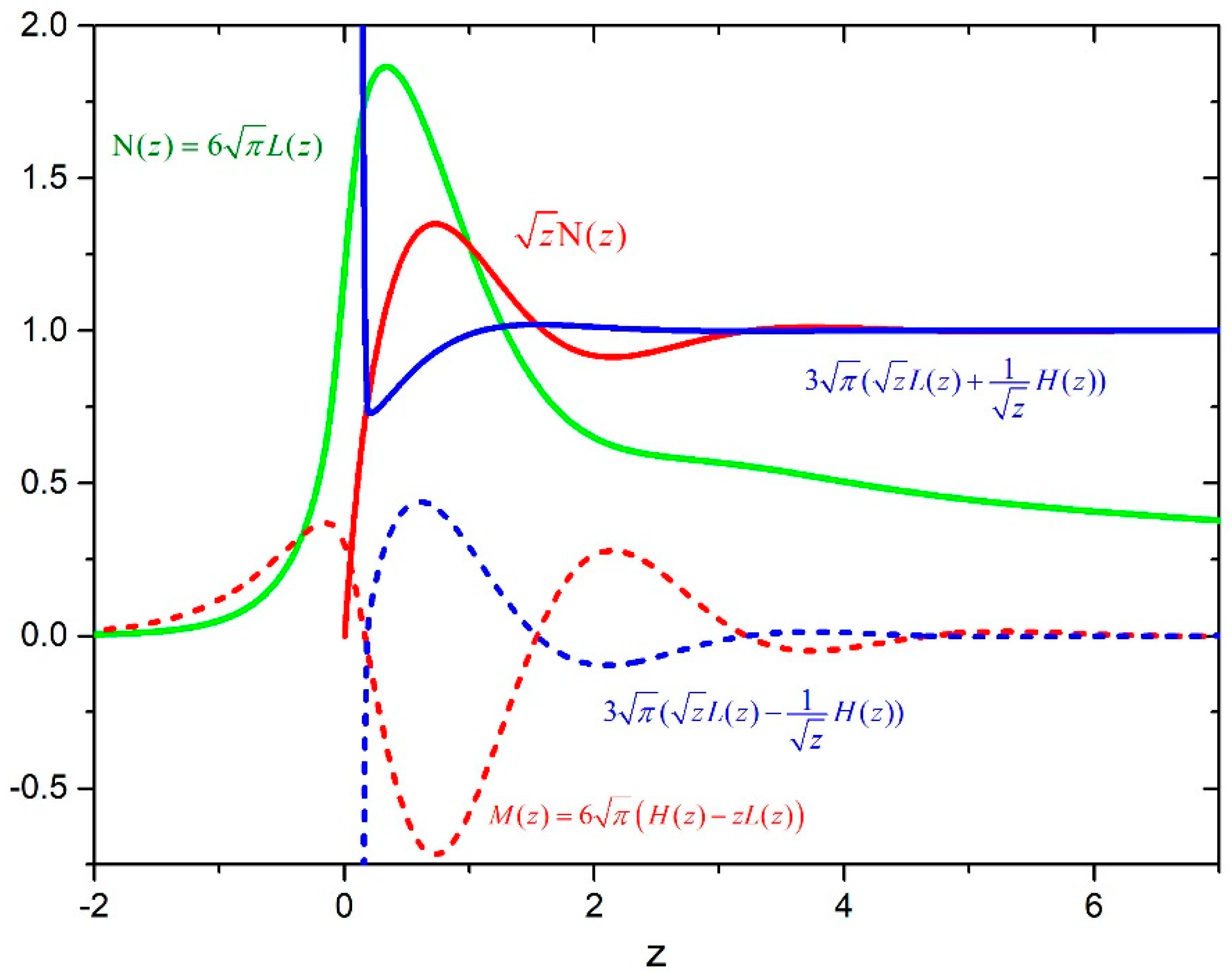
In the analysis of the $Li-He$ spectra we used the G. Peach ab initio calculation presented in Reference [21] (Figure 2a). $X{}^2\mathsf{\Sigma }$ and $B{}^2\mathsf{\Sigma }$ states had repulsive potentials with very small minima of (R_e = 11.73 a_o, D_e = 1.53741 cm⁻¹) and (R_e = 16.4785 a_o, D_e = 0.576 cm⁻¹), respectively. $A{}^2\mathsf{\Sigma }$ potential had a minimum (R_e = 3.33 a_o, D_e = 1061.33 cm⁻¹, ${\omega }_e=288.98{\mathrm{cm}}^{-1}$, B_e = 1.82 cm⁻¹). $A{}^2\mathsf{\Sigma }\to X{}^2\mathsf{\Sigma }$ transition had a monotonic difference potential forming a red wing of $2P_{3/2,1/2}\to 2S_{1/2}$ resonant doublet. The difference potential of the $B{}^2\mathsf{\Sigma }\to X{}^2\mathsf{\Sigma }$ transition had a maximum (V_m = 20645.6 cm⁻¹ at R_m = 3.70314 a_o), which corresponded to the satellite band at 484.364 nm in the blue wing of the resonant doublet.

For the absorption spectra calculation of the $L{i}_2$ molecule we used the Schmidt-Mink [22] ab initio calculation (Figure 2b). There were two ground states; the strongly bound $X{}^1\mathsf{\Sigma }{}_g^{+}$ state ($R_e=5.0a_o$, $D_e=8460.8{\mathrm{cm}}^{-1}$, ${\omega }_e=346.4{\mathrm{cm}}^{-1}$, $B_e=0.67{\mathrm{cm}}^{-1}$) and the $a{}^3\mathsf{\Sigma }{}_u^{+}$ state with a shallow minimum ($R_e=7.8a_o$, $D_e=324.0{\mathrm{cm}}^{-1}$, ${\omega }_e=57.4{\mathrm{cm}}^{-1}$, $B_e=0.26{\mathrm{cm}}^{-1}$). The excited $A{}^1\mathsf{\Sigma }{}_u^{+}$ state had a deep minimum ($R_e=5.9a_o$, $D_e=9345.3{\mathrm{cm}}^{-1}$, ${\omega }_e=252.9{\mathrm{cm}}^{-1}$, $B_e=0.49{\mathrm{cm}}^{-1}$) and the $A{}^1\mathsf{\Sigma }{}_u^{+}\to X{}^1\mathsf{\Sigma }{}_g^{+}$ difference potential had a minimum ($R_m=8.3a_o$, $V_m=10956.9{\mathrm{cm}}^{-1}$, ${\lambda }_m=912.6\mathrm{nm}$). The $B{}^1\mathsf{\Pi }{}_u$ state had two extremes, being a deep minimum ($R_e=5.5a_o$, $D_e=3390.6{\mathrm{cm}}^{-1}$, ${\omega }_e=263.9{\mathrm{cm}}^{-1}$, $B_e=0.54{\mathrm{cm}}^{-1}$) and a maximum (“hump”) at $R_h=12.0a_o$, with the energy 490.4cm⁻¹ above the asymptote. Transition $B{}^1\mathsf{\Pi }{}_u\to X{}^1\mathsf{\Sigma }{}_g^{+}$ had a monotonic difference potential. The excited triplet $b{}^3\mathsf{\Sigma }{}_g^{+}$ had a deep minimum ($R_e=6.0a_o$, $D_e=7032.4{\mathrm{cm}}^{-1}$, ${\omega }_e=245.9{\mathrm{cm}}^{-1}$, $B_e=0.5{\mathrm{cm}}^{-1}$) and the $b{}^3\mathsf{\Sigma }{}_g^{+}\to a{}^3\mathsf{\Sigma }{}_u^{+}$ difference potential had a minimum ($R_m=4.5a_o$, $V_m=6146.8{\mathrm{cm}}^{-1}$, ${\lambda }_m=1626.8\mathrm{nm}$). The $c{}^3\mathsf{\Pi }{}_g$ state had a repulsive potential energy curve but the difference potential of the $c{}^3\mathsf{\Pi }{}_g\to a{}^3\mathsf{\Sigma }{}_u^{+}$ transition had two close extremes, a minimum ($R_m=5.2a_o$, $V_m=16376.3{\mathrm{cm}}^{-1}$, ${\lambda }_m=610.6\mathrm{nm}$) and a maximum ($R_m=7.4a_o$, $V_m=16724.9{\mathrm{cm}}^{-1}$, ${\lambda }_m=597.9\mathrm{nm}$).

In the case of the $C{s}_2$ molecule we used the Allouche et al. [23] ab initio calculation (Figure 2c). There were two ground states; the strongly bound $X{}^1\mathsf{\Sigma }{}_g^{+}(0_g^{+})$ state ($R_e=8.7a_o$, $D_e=3755.4{\mathrm{cm}}^{-1}$, ${\omega }_e=45.0{\mathrm{cm}}^{-1}$, $B_e=0.012{\mathrm{cm}}^{-1}$) and the $a{}^3\mathsf{\Sigma }{}_u^{+}(1_u,0_u^{+})$ state with a shallow minimum ($R_e=11.9a_o$, $D_e=281.3{\mathrm{cm}}^{-1}$, ${\omega }_e=10.8{\mathrm{cm}}^{-1}$, $B_e=0.0064{\mathrm{cm}}^{-1}$). The excited $A{}^1\mathsf{\Sigma }{}_u^{+}(0_u^{+})$ state had a deep minimum ($R_e=9.8a_o$, $D_e=5816.3{\mathrm{cm}}^{-1}$, ${\omega }_e=38.4{\mathrm{cm}}^{-1}$, $B_e=0.0095{\mathrm{cm}}^{-1}$) and the $A{}^1\mathsf{\Sigma }{}_u^{+}(0_u^{+})\to X{}^1\mathsf{\Sigma }{}_g^{+}(0_g^{+})$ difference potential had a minimum ($R_m=10.8a_o$, $V_m=8754.7{\mathrm{cm}}^{-1}$, ${\lambda }_m=1142.2\mathrm{nm}$). The $B{}^1\mathsf{\Pi }{}_u(1_u)$ state had two extremes, a deep minimum ($R_e=9.03a_o$, $D_e=2456.1{\mathrm{cm}}^{-1}$, ${\omega }_e=37.4{\mathrm{cm}}^{-1}$, $B_e=0.011{\mathrm{cm}}^{-1}$) and a maximum (“hump”) at $R_h=17.6a_o$, with the energy only 18.9 cm⁻¹ above the asymptote. Difference potential of the $B{}^1\mathsf{\Pi }{}_u(1_u)\to X{}^1\mathsf{\Sigma }{}_g^{+}(0_g^{+})$ transition had one maximum ($R_m=7.8a_o$, $V_m=13302.4{\mathrm{cm}}^{-1}$, ${\lambda }_m=751.7\mathrm{nm}$). The excited triplet $b{}^3\mathsf{\Sigma }{}_g^{+}(1_g)$ state had a deep minimum ($R_e=10.2a_o$, $D_e=3028.7{\mathrm{cm}}^{-1}$, ${\omega }_e=28.1{\mathrm{cm}}^{-1}$, $B_e=0.0086{\mathrm{cm}}^{-1}$) and the $b{}^3\mathsf{\Sigma }{}_g^{+}(1_g)\to a{}^3\mathsf{\Sigma }{}_u^{+}(1_u)$ difference potential was monotonic. The $c{}^3\mathsf{\Pi }{}_g(1_g)$ state potential energy curve had two extremes, a minimum ($R_e=9.4a_o$, $D_e=1401.9{\mathrm{cm}}^{-1}$, ${\omega }_e=58.7{\mathrm{cm}}^{-1}$, $B_e=0.01{\mathrm{cm}}^{-1}$) and a hump at $R_h=15.1a_o$, with energy 170.513cm⁻¹ above the asymptote. The difference potential of the $c{}^3\mathsf{\Pi }{}_g(1_g)\to a{}^3\mathsf{\Sigma }{}_u^{+}(1_u)$ transition had one maximum ($R_m=14.1a_o$, $V_m=10512.8{\mathrm{cm}}^{-1}$, ${\lambda }_m=826.8\mathrm{nm}$).

4.1. Absorption Spectra of Li-He Molecule

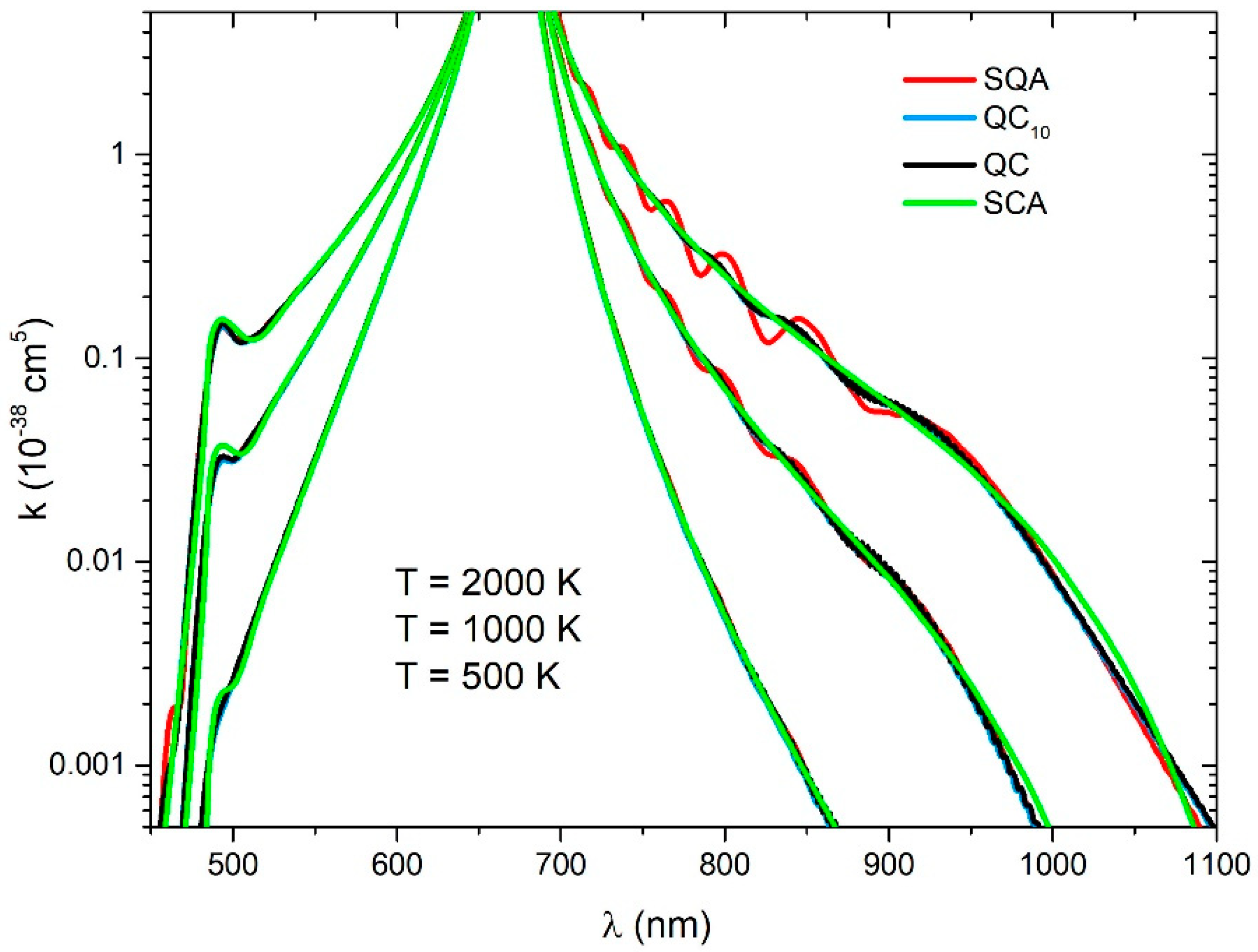
We found that using Equation (28) for $n\le 10$, there was a negligible difference between the QC and QC_n spectra. The number of grid points N = 370 was used. Spectra were collected in bins $\Delta \lambda =0.2\mathrm{nm}$ and smoothed with a Gaussian with half-width of 0.6 nm. In the calculation of the SQA spectra, the number of grid points N = 800 was used, and spectra are collected in the same bins, but smoothed with a Gaussian with half-with of 1.2 nm.

In the short-wavelength region (Figure 3) all the methods gave almost the same result. The SCA method showed small differences around the satellite band at 484.4 nm. In the long-wavelength region, where the Condon transitions are connected with the attractive well of $A{}^2\mathsf{\Sigma }$ state, Stückelberg oscillations occured which were consequence of the interference of the wave functions $X{}^2\mathsf{\Sigma }$ state near the turning point. These oscillations increased with temperature. At higher temperatures, there was a larger contribution of transitions starting from the ro-vibrational states of the $X{}^2\mathsf{\Sigma }$ state with high energy and turning points at a very steep ground state potential, where the interference effect was important. The SQA spectra showed much more pronounced oscillation because of the $J^{″}={\mathsf{\Lambda }}^{″}$ approximation, whilst they were smoothed in the QC and QC₁₀ by averaging over the $J^{″}$. There were no oscillations in the SCA spectra, whilst in this approach, the influence of a turning point close to the Condon points was neglected.

4.2. Absorption Spectra of Li₂ Molecule

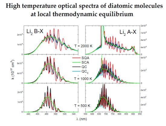
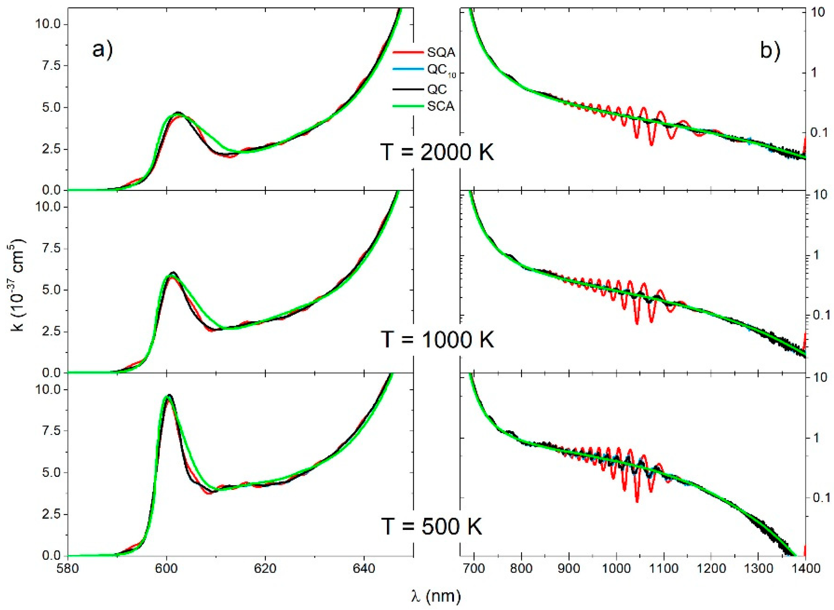
The number of grid points $N=400$ was used for the QC and QC_n, and $N=1000$ was used for the SQA spectra calculation. Using Equation (25) with $n\le 6$ there was negligible difference between the QC and QC_n spectra, so we compared the (Figure 4 and Figure 5) QC and QC₆ spectra. Ro-vibrational transitions were collected in bins $\Delta \lambda =0.2\mathrm{nm}$ and smoothed with a Gaussian with half-width of 0.6 nm (QC and QC₆) or a half-with 1.2 nm in the case of the SQA.

Spectra of the electronic $c{}^3\mathsf{\Pi }{}_g(1_g)\to a{}^3\mathsf{\Sigma }{}_u^{+}(1_u)$ transition (Figure 4a) contained mostly free–free ro-vibrational transitions. The main feature in these spectra was a satellite band around $597.9$ nm. The QC and QC₆ spectra had small oscillation at the lowest temperature, what can be considered the consequence of interference near the turning points of the repulsive $c{}^3\mathsf{\Pi }{}_g(1_g)$ state. At all temperatures, the SQA spectra had very small oscillation around the QC, but there was generally good agreement with the QC and with SCA as well.

The main contribution to the spectra of the electronic $b{}^3\mathsf{\Sigma }{}_g^{+}\to a{}^3\mathsf{\Sigma }{}_u^{+}$ transition (Figure 4b) came from the transitions between the free ro-vibrational states of the lower electronic state and the deeply bound ro-vibrational states of the upper electronic state. The QC and QC₆ continuous spectra had a shallow oscillatory structure as a consequence of the large vibrational energy differences in the upper electronic state (${\omega }_e=245.9{\mathrm{cm}}^{-1}$) and a decrease with the temperature. This oscillatory structure was overemphasized in SQA spectra, and it did not exist in the SCA spectra.

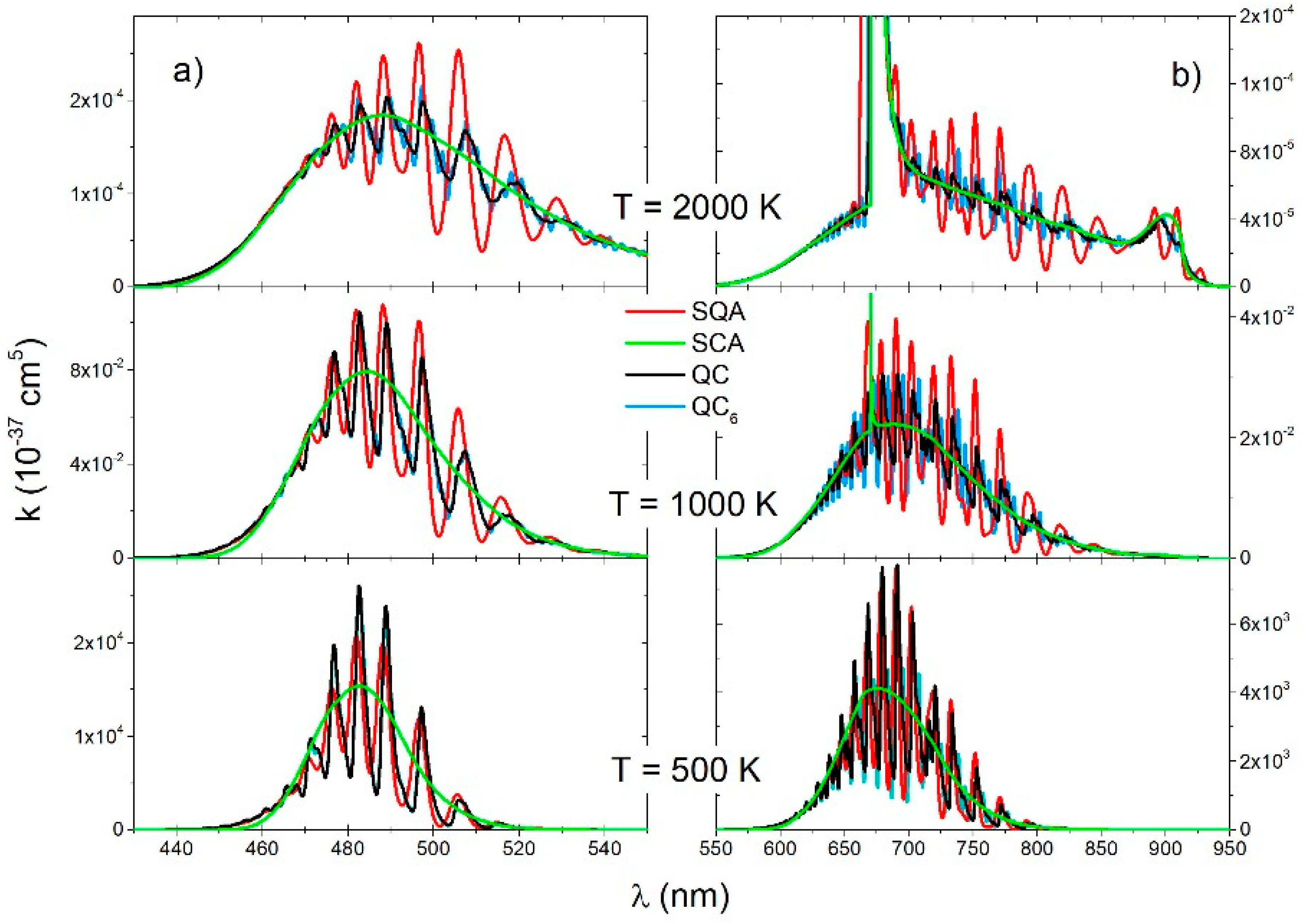
The QC and QC₆ spectra of the $B{}^1\mathsf{\Pi }{}_u\to X{}^1\mathsf{\Sigma }{}_g^{+}$ (Figure 5a) and $A{}^1\mathsf{\Sigma }{}_u^{+}\to X{}^1\mathsf{\Sigma }{}_g^{+}$ transition (Figure 5b) were roughly identical showing a strong vibrational band structure. The SQA spectra also had this vibrational band structure and at the lowest temperature of 500 K was in good agreement with the QC spectra. At higher temperatures, especially at 2000 K, the SQA did not give satisfactory results. The SCA spectra at all temperatures have good envelope of the QC spectra, especially at 2000 K, where quite right show shape of satellite band at ${\lambda }_m=912.6$ nm.

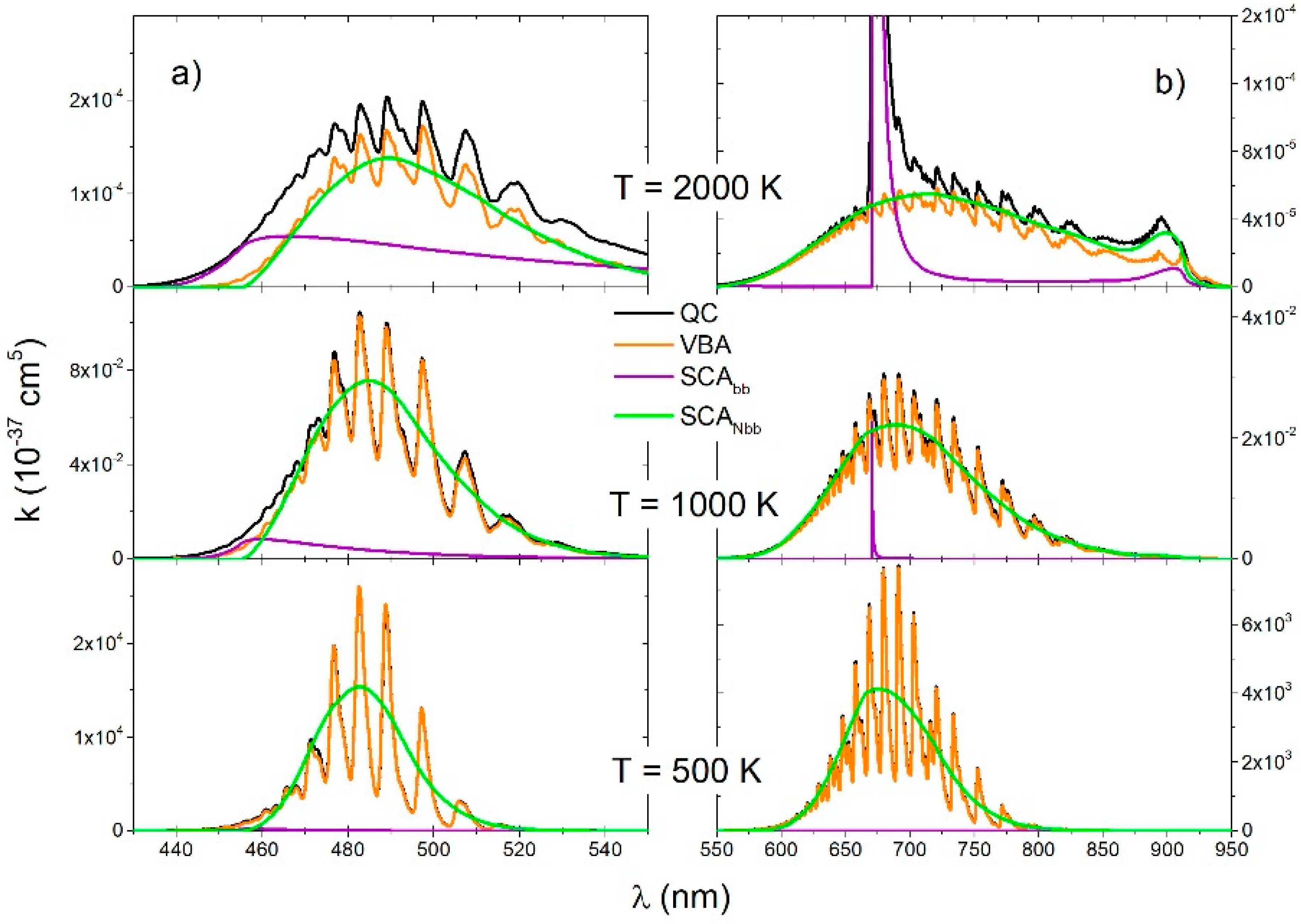
The QC spectra of the $B{}^1\mathsf{\Pi }{}_u\to X{}^1\mathsf{\Sigma }{}_g^{+}$ transition (Figure 6a) and the $A{}^1\mathsf{\Sigma }{}_u^{+}\to X{}^1\mathsf{\Sigma }{}_g^{+}$ transition (Figure 6b) was compared with the VBA spectra and two semiclassical spectra: SCA_bb and SCA_Nbb. Firstly, the SCA_bb is a spectrum of bound–bound transitions and the second one SCA_Nbb is a spectrum of free–free and free–bound transitions. Contribution of the free–free and free–bound transitions was negligible at T = 500 K, but it increased with temperature and was a dominant contribution in the near wings of the Li resonant line (Figure 6b). At the lowest temperature, the VBA was in perfect agreement with the QC because at that temperature a spectrum is completely of the bound–bound type. At 1000 K, there was also good matching between the SCA and VBA, except in the short wavelength region of the B-X transition.

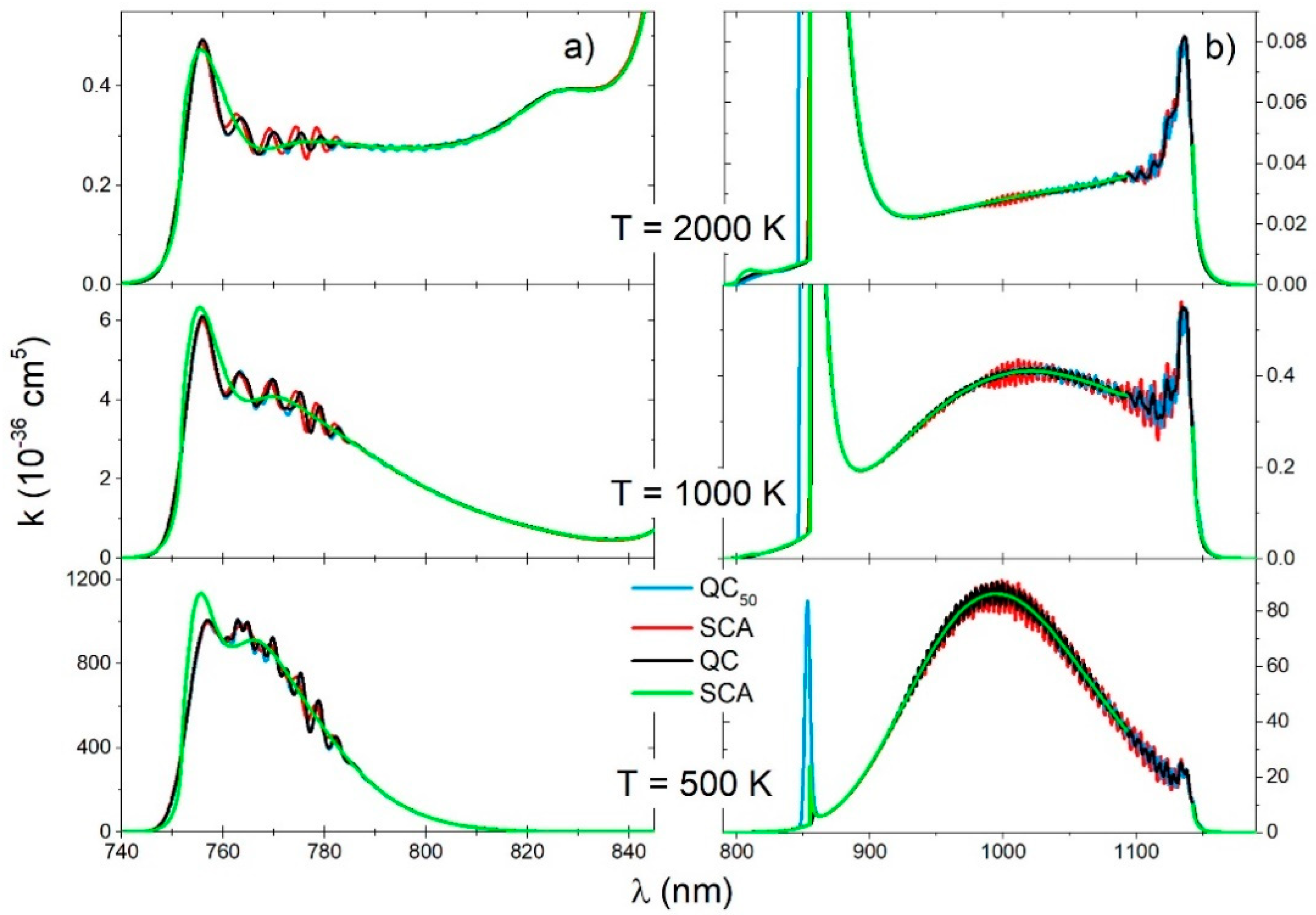
4.3. Absorption Spectra of Cs₂ Molecule

In the case of the $C{s}_2$ spectra we used $N=1400$ grid points for the QC, QC_n, and SQA spectra calculations. We found that that for $n\le 50$, the difference between the QC and QC_n was negligible. Spectral transitions were collected in bins $\Delta \lambda =0.2\mathrm{nm}$ and smoothed with a Gaussian with half-width of 0.6 nm (for QC, QC₅₀, SQA).

In the case of the continuous spectra of $c{}^3\mathsf{\Pi }{}_g(1_g)\to a{}^3\mathsf{\Sigma }{}_u^{+}(1_u)$ (Figure 7a) and the $b{}^3\mathsf{\Sigma }{}_g^{+}(1_g)\to a{}^3\mathsf{\Sigma }{}_u^{+}(1_u)$ electronic transition (Figure 7b), all of the investigated methods (QC, QC50, SQA, SCA) yielded results that were in excellent agreement amongst themselves. However, there was some deviation of the SCA in the neighborhood of the satellite band at ${\lambda }_m=826.8\mathrm{nm}$, for the lower temperatures.

Molecular bands spectra of the $B{}^1\mathsf{\Pi }{}_u(1_u)\to X{}^1\mathsf{\Sigma }{}_g^{+}(0_g^{+})$ (Figure 8a) and $A{}^1\mathsf{\Sigma }{}_u^{+}(0_u^{+})\to X{}^1\mathsf{\Sigma }{}_g^{+}(0_g^{+})$ electronic transitions (Figure 8b) showed the excellent agreement of the three approaches (SQA, QC₅₀, QC). Only the SCA approach could not show the discrete vibrational structure of the bands. That was the main reason for disagreement in this approach and the other approaches in the neighborhood of the satellite band at ${\lambda }_m=751.7\mathrm{nm}$.

5. Discussion and Conclusions

The use of a fully quantum-mechanical procedure based on the Fourier grid Hamiltonian method is a numerically robust but a time-consuming method. The most time-consuming part of the computation is the diagonalization of the Hamiltonian matrix. The time needed for this task depends on the number of grid points N, the form of matrix itself, the numerical algorithm and it is approximately $t=\alpha N^2\sqrt{N}$, ($\alpha$ is a number depending on computer and algorithm). The number of points must be larger than the number of bound states (if the potential of the electronic state is attractive) to have enough states which represent free states. To produce spectra which are correct at the frequencies corresponding to the transitions near the dissociation limit, the last grid point $R_N$ must be chosen so that the energy difference $V\left(R_N\right)-V(\infty )$ is small (where $V(R)$ is the energy of the electronic state). The number of grid points increased with the reduced mass of molecule $N=R_N\frac{\sqrt{2\mu E_T}}{\hslash }$, so we used N = 370, 400, 1400 for Li-He, Li₂, and Cs₂, respectively. To calculate all transition elements of the matrix P defined by $P(\nu ,T,n)$ (Equation (28)), one needs time $t=\alpha N^3\sqrt{N}/n$. The number of J-values collected in one transition in Equation (28) depended on the spectral resolution and interval between the rotational transitions which was proportional with $J^{″}\left(B_{v^{\prime }{\mathsf{\Lambda }}^{\prime }}-B_{v^{″}{\mathsf{\Lambda }}^{″}}\right)$. Given the B-constant is reciprocal to the reduced mass of the molecule, the number n increases with the mass and we used n = 10, 6, 50 for Li-He, Li₂, and Cs₂, respectively. To calculate the spectra QC or QC_n using Equation (36) one needs to collect all the transitions in bins of $\Delta \lambda$, i.e., what needs a time proportional to the number of transitions $t=\beta N^3/n$ ($\beta$ is number depending on computer and algorithm). It is important to emphasize that there is a relation for the time proportionality factors: $\alpha >>\beta$.

The Vibrational band approximation (VBA) was numerically time efficient because one needs only one Hamiltonian matrix diagonalization for the upper ${\mathsf{\Lambda }}^{\prime }$ and lower ${\mathsf{\Lambda }}^{″}$ electronic state. This approach gave good results for low temperatures, where the transitions between the lowest vibrational states gave the dominant contribution. For high temperatures, higher vibrational levels must be considered, where the energy difference between the adjacent vibrational states was decreasing and the first order perturbation approach for the ro-vibrational energies and wave functions was no longer applicable. Moreover, it is important to note that the VBA only gives the contribution of bound–bound transition to the spectra. As a consequence, in the case of the Li₂ molecule, VBA was in good agreement with the QC spectra of the A-X and B-X band at lower temperatures. VBA was not suitable for spectra of molecules with small ${\omega }_e$ like the $C{s}_2$ molecule, but it was an excellent theoretical tool to analyze the spectra of molecules with large ${\omega }_e$ of order ${10}^3$ cm⁻¹, such as N₂, O₂, and CO molecules as an example.

Semi-quantum approximation the SQA was also numerically time-efficient because it needed only one diagonalization of the Hamiltonian matrix for $J^{″}={\mathsf{\Lambda }}^{″}$. SQA gave good results if the interval between the rotational transitions was much smaller than the width of the instrumental profile, what is better satisfied in the case of molecules with larger reduced mass. To have enough states representing free molecular states, the number of grid points $N_S$ can be larger than number of points in the case of a full quantum calculation $N_S\ge N$. In our calculation, we used $N_S$ = 800, 1000, 1400 for Li-He, Li₂, and Cs₂, respectively. To calculate all transition elements of the matrix P (Equation 30) one needs time $t_S=\alpha N_S^2\sqrt{N_S}$. The ratio of times needed to calculate all transitions in the QC_n and SQA is $\frac{t}{t_S}=\frac{N}{n}{\left(\frac{N}{N_s}\right)}^{5/2}$. To calculate the spectra SQA using Equation (36) by collecting all the transitions in bins of $\Delta \lambda$, one needs time $t=\beta N^2$. The ratio of evaluation times of the QC_n, and SQA spectra was $\frac{t}{t_S}=\frac{N}{n}{\left(\frac{N}{N_s}\right)}^2$. The semi-quantum approximation was in very good agreement with the fully quantum calculations, whilst its computer time consumption could be lower by few orders of magnitude; in the case of the Cs₂ molecule SCA is 28 times faster than the QC₅₀ and 1400 times faster than the QC. A disadvantage of this method is an unsatisfactory description of the discrete rotational structure of the molecular bands and in some cases of the free–free spectra the overemphasis of interference effects in the neighborhood of turning points.

The standard semi-classical approximation SCA and its refinement, the uniform Airy approximation, did not give the ro-vibrational structure of the molecular bands, neglected the effects of turning points, but agreed with the averaged quantum-mechanical spectra and was computationally time efficient. Moreover, using the SCA it was possible to estimate contributions of the bound–bound, bound–free, and free–free transition to the spectra. “Semi-classical theory will also play an increasingly important role in interpreting the results of large, completely quantum mechanical calculations that are becoming increasingly feasible as a result of enhanced computer power” (W. H. Miller [24]).

Comparison of the experimental and theoretical absorption and emission spectra of diatomic molecules is an excellent tool for checking the accuracy of a molecular electronic structure: potential curves and transition dipole moments which are important data for plasma science. In the case of high density and high temperature plasma conditions, the assumption of thermal equilibrium is essential for an easy spectral simulation. Even in that case, different theoretical approaches are possible for a rapid spectral simulation and for comparison with experimental spectra. These spectral simulations could be applied even in non-thermal plasma conditions, which are probably more important for some applications, like new plasma sources, plasma diagnostics, thermal plasma theory, and materials science applications [25].

References

- Lam, L.K.; Gallagher, A.; Hessel, M.M. The intensity distribution in the Na 2 and Li 2 A—X bands. J. Chem. Phys. 1977, 66, 3550–3556. [Google Scholar] [CrossRef]
- Chung, H.-K.; Kirby, K.; Babb, J.F. Theoretical study of the absorption spectra of the lithium dimer. Phys. Rev. A 1999, 60, 2002–2008. [Google Scholar] [CrossRef] [Green Version]
- Chung, H.-K.; Kirby, K.; Babb, J.F. Theoretical study of the absorption spectra of the sodium dimer. Phys. Rev. A 2001, 63, 1–8. [Google Scholar] [CrossRef]
- Horvatić, B.; Beuc, R.; Movre, M. Numerical simulation of dense cesium vapor emission and absorption spectra. Eur. Phys. J. D 2015, 69, 113. [Google Scholar] [CrossRef]
- Veza, D.; Beuc, R.; Milošević, S.; Pichler, G. Cusp satellite bands in the spectrum of Cs2 molecule. Eur. Phys. J. D 1998, 2. [Google Scholar] [CrossRef]
- Bichoutskaia, E.; Devdariani, A.; Ohmori, K.; Misaki, O.; Ueda, K.; Sato, Y. Spectroscopy of quasimolecular optical transitions: Ca(4s2 1S0 ↔ 4s4p 1P, 4s3d 1D2)–He. The influence of radiation width. J. Phys. B 2001, 34, 2301–2312. [Google Scholar] [CrossRef]
- Hedges, R.; Drummond, D.L.; Gallagher, A. Extreme-Wing Line Broadening and Cs-Inert-Gas Potentials. Phys. Rev. A 1972, 6, 1519–1544. [Google Scholar] [CrossRef]
- Connor, J.N.L. Asymptotic evaluation of multidimensional integrals for the S matrix in the semiclassical theory of inelastic and reactive molecular collisions. Mol. Phys. 1973, 25, 181–191. [Google Scholar] [CrossRef]
- Connor, J.N.L.; Marcus, R.A. Theory of Semiclassical Transition Probabilities for Inelastic and Reactive Collisions. II Asymptotic Evaluation of the S Matrix. J. Chem. Phys. 1971, 55, 5636–5643. [Google Scholar] [CrossRef]
- Beuc, R.; Horvatic, V. The investigation of the satellite rainbow in the spectra of diatomic molecules. J. Phys. B 1992, 25, 1497–1510. [Google Scholar] [CrossRef]
- Vicharelli, P.A.; Collins, C.B. Uniform semiclasical description of satellite bands. In Spectral Line Shapes; Burnett, K., Ed.; De Gruyter: Berlin, Germany, 1983; Volume 2, pp. 537–549. [Google Scholar]
- Szudy, J.; Baylis, W.E. Unified Franck-Condon treatment of pressure broadening of spectral lines. J. Quant. Spectrosc. Radiat. Transf. 1975, 15, 641–668. [Google Scholar] [CrossRef]
- Sando, K.M.; Wormhoudt, J.C. Semiclassical Shape of Satellite Bands. Phys. Rev. A 1973, 7, 1889–1898. [Google Scholar] [CrossRef]
- Beuc, R.; Horvatić, B.; Movre, M. Semiclassical description of collisionally induced rainbow satellites: A model study. J. Phys. B 2010. [Google Scholar] [CrossRef]
- Devdariani, A.; Dalimier, E. Radiative characteristics of quasimolecular state interactions. Phys. Rev. A 2008, 78, 022512. [Google Scholar] [CrossRef]
- Colbert, D.T.; Miller, W.H. A novel discrete variable representation for quantum mechanical reactive scattering via the S -matrix Kohn method. J. Chem. Phys. 1992, 96, 1982–1991. [Google Scholar] [CrossRef]
- Willner, K.; Dulieu, O.; Masnou-Seeuws, F. Mapped grid methods for long-range molecules and cold collisions. J. Chem. Phys. 2004, 120, 548–561. [Google Scholar] [CrossRef] [PubMed]
- Beuc, R.; Movre, M.; Horvatić, B. Time-efficient numerical simulation of diatomic molecular spectra. Eur. Phys. J. D 2014, 68. [Google Scholar] [CrossRef]
- Patch, R.W.; Shackleford, W.L.; Penner, S.S. Approximate Spectral Absorption Coefficient Calculations for Electronic Band Systems Belonging to Diatomic Molecules. J. Quant. Spectrosc. Radiat. Transf. 1962, 2, 263–271. [Google Scholar] [CrossRef]
- Erdman, P.S.; Larson, C.W.; Fajardo, M.; Sando, K.M.; Stwalley, W.C. Optical absorption of lithium metal vapor at high temperatures. J. Quant. Spectrosc. Radiat. Transf. 2004, 88, 447–481. [Google Scholar] [CrossRef]
- Beuc, R.; Peach, G.; Movre, M.; Horvatić, B. Lithium, sodium and potassium resonance lines pressure broadened by helium atoms. Astron. Astrophys. Trans. 2018, 30, 315–322. [Google Scholar]
- Schmidt-Mink, I.; Müller, W.; Meyer, W. Ground- and excited-state properties of Li2 and Li2+ from ab initio calculations with effective core polarization potentials. Chem. Phys. 1985, 92, 263–285. [Google Scholar] [CrossRef]
- Allouche, A.-R.; Aubert-Frécon, M. Transition dipole moments between the low-lying states of the Rb2 and Cs2 molecules. J. Chem. Phys. 2012, 136, 114302. [Google Scholar] [CrossRef] [PubMed]
- Miller, W.H. Semiclassical methods in chemical physics. Science 1986, 233, 171–177. [Google Scholar] [CrossRef] [PubMed]
- Adamovich, I.; Baalrud, S.D.; Bogaerts, A.; Bruggeman, P.J.; Cappelli, M.; Colombo, V.; Czarnetzki, U.; Ebert, U.; Eden, J.G.; Favia, P.; et al. The 2017 Plasma Roadmap: Low temperature plasma science and technology. J. Phys. D Appl. Phys. 2017, 50, 323001. [Google Scholar] [CrossRef] [Green Version]
Figure 1.
Behavior of functions , , , , and .
Figure 2.
Potential curves of the lowest electronic states of the (a) molecule, (b) molecule, and (c) molecule. The electronic transition difference potential curves are given by dotted lines.
Figure 3.
reduced absorption coefficient for the (left) and transitions (right) for three different temperatures (2000 K, 1000 K, 500 K), obtained with four theoretical approaches (SQA, QC10, QC, SCA).
Figure 4.
molecule, reduced absorption coefficient for the (a) and (b) transitions for three different temperatures (2000 K, 1000 K, 500 K), obtained with four theoretical approaches (SQA, QC6, QC, SCA).
Figure 5.
molecule, reduced absorption coefficient for the (a) and transitions (b) for three different temperatures (2000 K, 1000 K, 500 K), obtained with four theoretical approaches (SQA, QC6, QC, SCA).
Figure 6.
molecule, reduced absorption coefficient for the (a) and (b) transitions for three different temperatures (2000 K, 1000 K, 500 K), obtained with four theoretical approaches (QC, VBA, SCAbb, SCANbb).
Figure 7.
molecule, (a) reduced absorption coefficient for the and (b) transitions for three different temperatures (2000 K, 1000 K, 500 K), obtained with four theoretical approaches (SQA, QC50, QC, SCA).
Figure 8.