Electron Scattering Processes in Non-Monochromatic and Relativistically Intense Laser Fields

Abstract

The theoretical analysis of four fundamental laser-assisted non-linear scattering processes are summarized in this review. Our attention is focused on Thomson, Compton, Møller and Mott scattering in the presence of intense electromagnetic radiation. Depending on the phenomena under considerations, we model the laser field as a single laser pulse of ultrashort duration (for Thomson and Compton scattering) or non-monochromatic trains of pulses (for Møller and Mott scattering).

1. Introduction

Scattering theory is the part of theoretical physics in which interactions of particles and waves are investigated at remote times and large distances, as compared with typical time and size scales of probed systems. For this reason, scattering theory is the most effective and, in many cases, the only method of analyzing such diverse systems as the micro-world or the whole universe. Not surprisingly, the investigation of scattering phenomena has been playing a central role in physics since the end of the nineteenth century, starting from the Rayleigh’s explanation of why the sky is blue, up to modern medical applications of computerized tomography, the very recent discovery of the Higgs particle and the detection of gravitational waves. A general analysis of quantum and classical scattering phenomena can be found in numerous textbooks. Among them, we refer the reader to Refs. [1,2,3,4,5].

Scattering processes played a fundamental role in the development of science from the theoretical and experimental points of view. For instance, it was the analysis of alpha particle collisions with thin metallic sheets that allowed Rutherford to discover the atomic nucleus. In 1912, the Austrian physicist V. F. Hess detected an ionizing radiation, the intensity of which increased with altitude. It seemed to originate beyond the atmosphere upper boundaries (for a detailed historical perspective, we refer the reader to Refs. [6,7]). Those particular rays, more penetrating than $\gamma$ radiation, were initially named ultra-rays and are now known as cosmic rays [8]. For his work in this field, Hess was awarded the Nobel Prize in physics in 1936, which he shared with C. D. Anderson (discoverer of the positron) [9]. However, the nature and origin of those rays was subject of great controversy. It was first assumed that the ultra-radiation was of electromagnetic origin (photons) due to its unique ability to penetrate matter (see Compton’s article on this subject [10]). On the other hand, W. Bothe and W. Kolhörster [11], by making simultaneous measurements in a stack of multiple detectors, found evidence that cosmic rays behave in certain aspects as very energetic charged particles [7,10]. In that case, the magnetic field surrounding our planet would have a considerable effect on the trajectories followed by the radiation. Namely, IT would be expected to observe a higher radiation intensity near the Earth’s poles than in the vicinity of the equator (the so-called latitude effect). This was experimentally demonstrated by J. Clay, who compared the intensity of cosmic rays measured at the island of Java and in northern Europe, and was later confirmed by several scientific expeditions around the globe [10]. Hence, it became commonly accepted that the conspicuous ultra-rays and the well-known β-radiation share, in principle, the same nature. It is not surprising that the stopping mechanism of relativistic electrons became a central topic in the early 1930s; the understanding of cosmic rays and their interaction with matter and its constituents was a focus of the scientific research. Furthermore, the stopping process of less-energetic electrons was of great interest in the studies of radioactivity and the ultimate composition of matter [12,13]. Note that only a few years earlier, in 1928, Dirac had published his prominent equation, which determines the evolution of quantum particles (or antiparticles) from a relativistic perspective. This, in turn, provided an invaluable tool for the early research in relativistic quantum mechanics. Since the discovery of the electron by J. J. Thomson and the atomic nucleus by Rutherford, it was clear that the stopping process should be reduced to two fundamental events: relativistic electron scattering by nuclei and by other electrons present in matter. To this end, the application of the recently formulated Dirac equation was necessary. It was Sir Nevill Francis Mott [14] who in 1929 addressed the first problem in the article “The scattering of fast electrons by atomic nuclei”, where he presented his celebrated scattering formula. The second problem was analyzed by the Danish physicist Christian Møller [15,16] during 1931–1932, who also derived a scattering formula for the relativistic collision of two electrons.

Another phenomenon of fundamental importance for the understanding of classical electromagnetism and the rising quantum theory was electron scattering by electromagnetic fields. This was first analyzed by J. J. Thomson [17], following the discovery of his charged corpuscles, now known as electrons. He considered a charged particle in the presence of an oscillating electromagnetic field. According to classical mechanics, such particle should be subject to time-dependent forces leading to its acceleration. This, in turn, would cause the emission of a secondary radiation with the exact same frequency as the incident one. Thomson’s point of view was vastly accepted among the scientific community at that time. However, increasing experimental evidence concerning the scattering of γ- or hard X-rays by electrons pointed out a consistent deviation from classical predictions (see the discussion in Ref. [18]). The application of quantum theory to this particular problem came in 1923 with A. H. Compton’s article “A quantum theory of the scattering of X-rays by light elements” [19]. In this article, besides the novel theoretical approach to scattering, the author presented compelling experimental evidence supporting his theory.

Arguably, one of the most important inventions in the second half of the 20th century was the laser. Early laser systems provided a unique source of monochromatic and coherent electromagnetic radiation. For this reason, in the 1960s, one can observe a revival in fundamental investigations concerning electron scattering processes (Thomson, Compton, Mott and Møller scattering) in the presence of light fields. Those early works focused predominantly on the influence of the electromagnetic radiation on scattering cross-sections, and the possibility of photon absorption (or emission) by the electron. Later on, the high light intensities generated by lasers made it necessary to divide the scattering events as linear (simultaneous absorption of single photons) or non-linear (simultaneous absorption of multiple photons) phenomena. Note that many of the theoretical analyses developed during the period of 1960–2000 considered long-in-time laser pulses, and the monochromatic (or quasi-monochromatic) plane-wave field approximation was commonly used. However, since the invention of the chirped-pulse amplification (CPA) technique by D. Strickland and G. Mourou [20] (they, together with A. Ashkin, shared the Nobel Prize in physics in 2018 [21]), it became possible to obtain ultraintense laser pulses of ultrashort duration. For this reason, in the previous decade, the non-linear electron scattering assisted by ultrashort light pulses received considerable attention.

It is the aim of the present review to give a theoretical (and historical) perspective of the fundamental electron scattering process in the presence of intense electromagnetic radiation. We present the results, previously obtained by some of us, for the laser-assisted Thomson, Compton, Møller and Mott scattering. Depending on the problem under consideration, two types of laser fields are considered: single ultrashort and finite light pulses, or infinite trains of temporally-shaped pulses. Special emphasis is put on the calculation of the corresponding probability amplitudes and the analysis of quantum resonances (when they are present). We also review the generalized Klein–Nishina formula for arbitrary shape of the laser pulses in the context of the Compton process.

This article is divided as follows. In Section 2, we analyze the classical and quantum evolution of electrons in the electromagnetic field. While Section 2.1 refers to the solution of the Newton-Lorentz equations and the identification of three independent invariants of motion (which fully define the behavior of the electron in the laser pulse), Section 2.2 presents the so-called relativistic Volkov states [22], i.e., the solutions of the Dirac equation in the electromagnetic field. The results obtained there are used to study the laser-assisted Thomson, Compton, Møller and Mott scattering (Section 3, Section 4, Section 5 and Section 6, respectively). In Section 4, we present a scaling law between Thomson and Compton frequencies of emitted radiation, for which the classical and quantum energy distributions coincide. This was previously done in Refs. [23,24,25,26]. Furthermore, the generalization of the Klein–Nishina formula for arbitrary laser pulses [27] is also presented there. For more information about the scattering phenomena for less general laser fields, we refer the reader to the 2009 review [28].

Throughout this paper, we use the metric $g^{\mu \nu }=\mathrm{diag}[1,-1,-1,-1]$ such that the scalar product between two arbitrary four-vectors a and b is $a·b=a^{\mu }{b}_{\mu }=a^0{b}^0-\mathit{a}·\mathit{b}$. The slashed notation is also used, i.e., $\cancel{a}={\gamma }^{\mu }{a}_{\mu }$, where ${\gamma }^{\mu }$ are the Dirac gamma matrices. Furthermore, the tensor ${\sigma }^{\mu \nu }$ is defined with respect to the commutator among those matrices, namely ${\sigma }_{\mu \nu }=\frac{\mathrm{i}}{2}[{\gamma }_{\mu },{\gamma }_{\nu }]$. For our calculations and formulas we use units where $\hslash =1$, c is the speed of light, $m_{\mathrm{e}}$ and $e=-\left|e\right|$ are the electron mass and charge, respectively.

2. Relativistic Free-Particles in the Laser Field

This section is devoted to the analysis of the temporal evolution of a relativistic, free-particle in a laser field. While the first part concerns a purely classical treatment, the second part is devoted to its quantum counterpart. In scattering theory it is assumed that, in the remote past and far future, the interacting particles are in free states. Hence, to study the light-assisted scattering phenomena, it is necessary to determine the behaviour of those free-states in the presence of electromagnetic radiation. Once the general properties and notation for such states are established, the laser-assisted scattering processes will be considered. Even though the phenomena presented in this section have been thoroughly analyzed (see, e.g., Refs. [29,30,31,32] for the classical treatment, and Refs. [33,34,35,36] for the quantum description), we make here a short overview of the most important results and methods.

2.1. Classical Solution

We are interested in analyzing the classical interaction of an electron with a finite-in-time laser pulse defined by the vector potential $\mathit{A}(\mathit{x},t)$ [32]. The oscillating magnetic and electric fields describing the pulse are given by $\mathcal{B}(\mathit{x},t)=\nabla \times \mathit{A}(\mathit{x},t)$ and $\mathcal{E}(\mathit{x},t)=-{\partial }_t\mathit{A}(\mathit{x},t)$, respectively. The light field propagates along the direction $\mathit{n}=\mathit{S}(\mathit{x},t)/\left|\mathit{S}\right(\mathit{x},t\left)\right|$ where $\mathit{S}(\mathit{x},t)=\mathcal{E}(\mathit{x},t)\times \mathcal{B}(\mathit{x},t)/{\mu }_0$ is the Poynting vector and ${\mu }_0$ is the permeability of free space. Furthermore, the electric and magnetic fields fulfill the relations $\mathcal{B}(\mathit{x},t)=\mathit{n}\times \mathcal{E}(\mathit{x},t)/c$ or $\mathcal{E}(\mathit{x},t)=c\mathcal{B}(\mathit{x},t)\times \mathit{n}$, where c is the speed of light. In the following, we assume that the plane-wave field approximation is valid, meaning that $\mathit{A}(\mathit{x},t)$ depends on the spatial and temporal coordinates only through the phase $\varphi =\omega t-\mathit{k}·\mathit{x}\equiv k·x=k^{\mu }{x}_{\mu }$, where $\left(x^{\mu }\right)=(ct,\mathit{x})$ is the space-time four vector, $\left(k^{\mu }\right)=(\omega /c,\mathit{k})=k^0(1,\mathit{n})=k^{0}n$ is the wave four-vector, $\omega$ relates to the frequency of oscillations, and $k^0=\omega /c$ is the wavenumber. It is also assumed that the laser pulse is finite and vanishes outside the interval $\varphi \in ]0,2\pi [$. For this reason, we define the vector potential $\mathit{A}(\mathit{x},t)\equiv \mathit{A}\left(\varphi \right)$ as

$$\mathit{A}\left(\varphi \right)=-\frac{1}{\omega }{\int }_0^{\varphi }\mathrm{d}\phi \mathcal{E}\left(\phi \right)$$

(1)

for $0<\varphi <2\pi$ and $\mathit{A}\left(\varphi \right)=\mathbf{0}$ otherwise. Note that, if $T_{\mathrm{p}}$ is the duration of the pulse, then $\omega =2\pi /T_{\mathrm{p}}$.

Let us now consider an electron of four momentum $\left(p^{\mu }\right)=(p^0,\mathit{p})$ and velocity $\mathit{v}=c\mathit{p}/p^0$ interacting with the laser field described above. Its temporal evolution, from the perspective of classical electrodynamics, is determined by the relativistic Newton-Lorentz equation of motion

$$\frac{\mathrm{d}\mathit{p}}{\mathrm{d}t}=e\mathcal{E}\left(\varphi \right)+e\mathit{v}\times \mathcal{B}\left(\varphi \right).$$

(2)

For our further purposes, it is convenient to write the magnetic component of the above expression in terms of $p$, $p^0$, and $\mathcal{E}\left(\varphi \right)$. In doing so, we obtain

$$\frac{\mathrm{d}\mathit{p}}{\mathrm{d}t}=\omega \left[1-\frac{\mathit{p}·\mathit{n}}{p^0}\right]\frac{\mathrm{d}\mathit{p}}{\mathrm{d}\varphi }=e\left[1-\frac{\mathit{p}·\mathit{n}}{p^0}\right]\mathcal{E}\left(\varphi \right)+e\frac{\mathit{p}·\mathcal{E}\left(\varphi \right)}{p^0}\mathit{n}.$$

(3)

According to Equation (3), the laser field acts differently along its direction of propagation and the plane perpendicular to it. Hence, it is natural to introduce the parallel and perpendicular components of the electron momentum with respect to $\mathit{n}$, defined as $p^{\parallel }=\mathit{p}·\mathit{n}$ and ${\mathit{p}}^{\perp }=\mathit{p}-p^{\parallel }\mathit{n}$, respectively. With this in mind, we write now the Newton-Lorentz equation as

$$\frac{\mathrm{d}\mathit{p}}{\mathrm{d}\varphi }=\frac{1}{\omega }e\mathcal{E}\left(\varphi \right)+\frac{1}{\omega (p^0-p^{\parallel })}\left[e\mathcal{E}\left(\varphi \right)·{\mathit{p}}^{\perp }\right]\mathit{n}.$$

(4)

Equation (4), together with appropriate initial conditions, contains all information necessary to determine the evolution of the electron in the laser field. However, it is worth mentioning that its validity is restricted by the plane-wave-front approximation for the laser field. In the following, we demonstrate that such equation leads to three independent invariants of motion which characterize the free-particle dynamics.

• First, we analyze the parallel component of momentum with respect to $\mathit{n}$. From Equation (4), it is evident that $p^{\parallel }$ satisfies the differential equation,

  $$\frac{\mathrm{d}{p}^{\parallel }}{\mathrm{d}\varphi }=\frac{e\mathcal{E}\left(\varphi \right)·{\mathit{p}}^{\perp }}{\omega (p^0-p^{\parallel })}.$$

  (5)
  Hence, using the on-mass-shell relation for the electron four-momentum, $p^{\mu }{p}_{\mu }={\left(p^0\right)}^2-{\mathit{p}}^2=m_{\mathrm{e}}^2{c}^2$, we obtain that

  $$\frac{\mathrm{d}{p}^0}{\mathrm{d}\varphi }=\frac{({\mathit{p}}^{\perp }+p^{\parallel }\mathit{n})}{p^0}·\frac{\mathrm{d}\mathit{p}}{\mathrm{d}\varphi }=\frac{e\mathcal{E}\left(\varphi \right)·{\mathit{p}}^{\perp }}{\omega (p^0-p^{\parallel })}.$$

  (6)
  By comparing Equations (5) and (6), we conclude that $p^0-p^{\parallel }$ is a conserved quantity during the interaction with the laser pulse, meaning that

  $$\frac{\mathrm{d}}{\mathrm{d}\varphi }(p^0-p^{\parallel })=0.$$

  (7)
  Therefore, the first invariant of motion, ${\mathrm{I}}_1$, is defined as

  $${\mathrm{I}}_1=p^0-p^{\parallel }.$$

  (8)
• From the Newton-Lorentz equation (Equation (4)), the perpendicular component of momentum ${\mathit{p}}^{\perp }$ obeys the relation,

  $$\frac{\mathrm{d}{\mathit{p}}^{\perp }}{\mathrm{d}\varphi }=\frac{e\mathcal{E}\left(\varphi \right)}{\omega }.$$

  (9)
  According to Equation (1), it is also possible to write the above relation in terms of the vector potential. In doing so, we obtain the second invariant of motion,

  $${\mathbf{I}}_2={\mathit{p}}^{\perp }+e\mathit{A}\left(\varphi \right),$$

  (10)

  which means that the canonical momentum of the electron, in the direction perpendicular to the laser field propagation, is conserved. It is worth mentioning that ${\mathbf{I}}_2$, as a vector, implicitly defines two independent relations. Thus, the three invariants are already determined by the set $\{{\mathrm{I}}_1,{\mathbf{I}}_2\}$.

In the following, we analyze the consequences derived from the invariants of motion defined above. Let us start by assuming that a free charged particle with initial momentum ${\mathit{p}}_{\mathrm{i}}$ interacts with the electromagnetic radiation at $\varphi =0$, i.e., $\mathit{p}(\varphi =0)={\mathit{p}}_{\mathrm{i}}$. According to ${\mathbf{I}}_2$ in Equation (10), after the laser pulse is over, the perpendicular momentum ${\mathit{p}}_{\mathrm{f}}^{\perp }\equiv {\mathit{p}}^{\perp }\left(2\pi \right)$ satisfies ${\mathit{p}}_{\mathrm{f}}^{\perp }+e\mathit{A}\left(2\pi \right)={\mathit{p}}_{\mathrm{i}}^{\perp }+e\mathit{A}\left(0\right)$. The vector potential vanishes at $\varphi =0$ and $\varphi =2\pi$, thus ${\mathit{p}}_{\mathrm{f}}^{\perp }$ must be equal to ${\mathit{p}}_{\mathrm{i}}^{\perp }$. Additionally, and taking into account that the four-momentum is on the mass shell, the invariant ${\mathrm{I}}_1$ in Equation (8) implies that $p_{\mathrm{i}}^{\parallel }=p_{\mathrm{f}}^{\parallel }$ and, therefore, $p_{\mathrm{i}}=p_{\mathrm{f}}$. In other words, the invariants of motion derived from the Newton-Lorentz equation result in the electron being neither accelerated nor decelerated by the action of the laser pulse, if treated in the plane-wave-front approximation. This is the so-called Lawson-Woodward theorem of no acceleration [37,38]. For our further purposes, we write another invariant by noting that the equation

$$\frac{\mathrm{d}}{\mathrm{d}\varphi }\left[\frac{1}{2}{\left({\mathit{p}}^{\perp }\right)}^2-p^{\parallel }(p^0-p^{\parallel })\right]=0,$$

(11)

is always satisfied. Hence, we define the “third” invariant in the following way,

$${\mathrm{I}}_3=p^{\parallel }(p^0-p^{\parallel })-\frac{1}{2}{\left({\mathit{p}}^{\perp }\right)}^2.$$

(12)

As one can check, the relation ${\mathrm{I}}_1^2+2{\mathrm{I}}_3=m_{\mathrm{e}}^2{c}^2$ is fulfilled, which means that ${\mathrm{I}}_1$ and ${\mathrm{I}}_3$ define the rest mass of the particle [32].

We construct now the trajectories $\mathit{x}\left(\varphi \right)$ followed by the electron, initially located at the position ${\mathit{x}}_{\mathrm{i}}$, in the light field. Let us also assume that the initial momentum of the particle, before the interaction with the laser pulse starts, is ${\mathit{p}}_{\mathrm{i}}={\mathit{p}}_{\mathrm{i}}^{\perp }+p_{\mathrm{i}}^{\parallel }\mathit{n}$. From the invariant ${\mathbf{I}}_2$ we have that

$${\mathit{p}}^{\perp }\left(\varphi \right)={\mathit{p}}_{\mathrm{i}}^{\perp }-e\mathit{A}\left(\varphi \right),$$

(13)

and, by making use of ${\mathrm{I}}_1$ and ${\mathrm{I}}_3$, we find that the parallel component $p^{\parallel }\left(\varphi \right)$ is given by

$$p^{\parallel }\left(\varphi \right)=p_{\mathrm{i}}^{\parallel }+\frac{{\left[{\mathit{p}}^{\perp }\left(\varphi \right)\right]}^2-{\left({\mathit{p}}_{\mathrm{i}}^{\perp }\right)}^2}{2(p_{\mathrm{i}}^0-p_{\mathrm{i}}^{\parallel })}=p_{\mathrm{i}}^{\parallel }+\frac{{[{\mathit{p}}_{\mathrm{i}}^{\perp }-e\mathit{A}\left(\varphi \right)]}^2-{\left({\mathit{p}}_{\mathrm{i}}^{\perp }\right)}^2}{2(p_{\mathrm{i}}^0-p_{\mathrm{i}}^{\parallel })}.$$

(14)

In our calculations, we have considered the independent variable as the phase of the laser field $\varphi$. Therefore, our aim is to represent the position of the particle as a function of such variable, namely, we want to calculate $\mathit{x}\left(\varphi \right)$. To this end, we use

$$\frac{\mathrm{d}}{\mathrm{d}t}=\frac{\omega (p^0-p^{\parallel })}{p^0}\frac{\mathrm{d}}{\mathrm{d}\varphi },$$

(15)

which directly implies that

$$\frac{\mathrm{d}\mathit{x}\left(\varphi \right)}{\mathrm{d}\varphi }=\frac{c}{\omega (p^0-p^{\parallel })}\mathit{p}\left(\varphi \right).$$

(16)

In other words, the perpendicular and parallel components of the “velocity” of the electron (as a function of $\varphi$) are given explicitly by

$$\begin{array}{cc}\hfill {{\mathit{x}}^{\prime }}^{\perp }\left(\varphi \right)& \equiv \frac{\mathrm{d}{\mathit{x}}^{\perp }\left(\varphi \right)}{\mathrm{d}\varphi }=\frac{c}{\omega (p^0-p^{\parallel })}[{\mathit{p}}_{\mathrm{i}}^{\perp }-e\mathit{A}\left(\varphi \right)],\hfill \end{array}$$

(17)

$$\begin{array}{cc}\hfill {x^{\prime }}^{\parallel }\left(\varphi \right)& \equiv \frac{\mathrm{d}{x}^{\parallel }\left(\varphi \right)}{\mathrm{d}\varphi }=\frac{c}{\omega (p^0-p^{\parallel })}\left[p_{\mathrm{i}}^{\parallel }-\frac{2e\mathit{A}\left(\varphi \right)·{\mathit{p}}_{\mathrm{i}}^{\perp }-e^2{\mathit{A}}^2\left(\varphi \right)}{2(p_{\mathrm{i}}^0-p_{\mathrm{i}}^{\parallel })}\right],\hfill \end{array}$$

(18)

where the “primes” denote the derivative $\mathrm{d}/\mathrm{d}\varphi$. Finally, according to Equations (17) and (18), we find that the classical trajectory described by the electron in a finite-in-time laser pulse is

$${\mathit{x}}^{\perp }\left(\varphi \right)={\mathit{x}}_{\mathrm{i}}^{\perp }+\frac{c}{\omega (p^0-p^{\parallel })}\left[{\mathit{p}}_{\mathrm{i}}^{\perp }\varphi -e{\int }_0^{\varphi }\mathrm{d}{\varphi }^{\prime }\mathit{A}\left({\varphi }^{\prime }\right)\right],$$

(19)

$$x^{\parallel }\left(\varphi \right)=x_{\mathrm{i}}^{\parallel }+\frac{c}{\omega (p^0-p^{\parallel })}\left[p_{\mathrm{i}}^{\parallel }\varphi -\frac{1}{2(p_{\mathrm{i}}^0-p_{\mathrm{i}}^{\parallel })}{\int }_0^{\varphi }\mathrm{d}{\varphi }^{\prime }\left[2e\mathit{A}\left({\varphi }^{\prime }\right)·{\mathit{p}}_{\mathrm{i}}^{\perp }-e^2{\mathit{A}}^2\left({\varphi }^{\prime }\right)\right]\right].$$

(20)

For the classical scattering, we define the space-time four vector as $x\left(\varphi \right)=\left(ct\right(\varphi ),\mathit{x}(\varphi \left)\right)$, with $\mathit{x}\left(\varphi \right)={\mathit{x}}^{\perp }\left(\varphi \right)+\mathit{n}{x}^{\parallel }\left(\varphi \right)$. For the sake of completeness, we also present here the equations defining the “acceleration” with respect to the phase, i.e.,

$$\begin{array}{cc}\hfill {{\mathit{x}}^{″}}^{\perp }\equiv \frac{{\mathrm{d}}^2{\mathit{x}}^{\perp }}{\mathrm{d}{\varphi }^2}& =-\frac{ec}{\omega (p^0-p^{\parallel })}\frac{\mathrm{d}\mathit{A}\left(\varphi \right)}{\mathrm{d}\varphi },\hfill \end{array}$$

(21)

$$\begin{array}{cc}\hfill {x^{″}}^{\parallel }\equiv \frac{{\mathrm{d}}^2{x}^{\parallel }}{\mathrm{d}{\varphi }^2}& =\frac{ce}{\omega {(p^0-p^{\parallel })}^2}(e\mathit{A}\left(\varphi \right)-{\mathit{p}}_{\mathrm{i}}^{\perp })·\frac{\mathrm{d}\mathit{A}\left(\varphi \right)}{\mathrm{d}\varphi }.\hfill \end{array}$$

(22)

These formulas are used in Section 3 when we analyze the Thomson scattering. Note that the treatment developed in this section comes from the fully relativistic analysis of the electron dynamics in the laser field.

2.2. Quantum Solution

From a quantum perspective, we consider now the temporal evolution of a charged, relativistic particle of four-momentum $p^{\mu }$ in the laser field. In our notation, the wave function describing such particle (or antiparticle) is represented by the bispinor ${\psi }_{\mathit{p}\lambda }^{\left(\beta \right)}\left(x\right)$ where $\beta =\pm$ labels the positive and negative energy solutions of the Dirac equation, and $\lambda =\pm$ determines the spin degrees of freedom. The electromagnetic radiation is defined by the four-vector potential $A^{\mu }\left(\varphi \right)=(0,\mathit{A}\left(\varphi \right))$. As we consider an arbitrary polarization of the laser field, the most general form of such potential is

$$\begin{array}{c}\hfill A\left(\varphi \right)=A_0[{\epsilon }_1{f}_1\left(\varphi \right)+{\epsilon }_2{f}_2\left(\varphi \right)]\equiv -\frac{\mu m_{\mathrm{e}}c}{e}[{\epsilon }_1{f}_1\left(\varphi \right)+{\epsilon }_2{f}_2\left(\varphi \right)].\end{array}$$

(23)

Here, we have introduced two arbitrary shape functions with continuous second derivatives $f_j\left(\varphi \right)$, $j=1,2$, the amplitude of the vector potential $A_0$, the relativistically invariant parameter $\mu =\left|e\right|A_0/m_{\mathrm{e}}c$, and two orthonormal polarization four-vectors ${\epsilon }_j^{\mu }=(0,{\mathit{\epsilon }}_j)$ such that ${\epsilon }_i^{\mu }{{\epsilon }_j}_{\mu }=-{\delta }_{ij}$ and $k^{\mu }{{\epsilon }_j}_{\mu }=0$. Note that, as the laser field is a propagating transverse wave, the relations $k·A=k^{\mu }{A}_{\mu }=0$ and $k^2=k·k=0$ always hold. The bispinor ${\psi }_{\mathit{p}\lambda }^{(+)}\left(x\right)$ describing an electron (particle) of momentum $\mathit{p}$ interacting with the electromagnetic radiation satisfies the Dirac equation in the laser field, namely,

$$\left(\mathrm{i}\cancel{\partial }-e\cancel{A}-m_{\mathrm{e}}c\right){\psi }_{\mathit{p}\lambda }^{(+)}\left(x\right)=0$$

(24)

and it is known as the Volkov solution (VS) [22]. To find an analytical expression for ${\psi }_{\mathit{p}\lambda }^{(+)}\left(x\right)$, Equation (24) has to be solved explicitly. As mentioned in Ref. [34], the VS for plane waves can be found by a variety of methods, including algebraic procedures, decoupling of the spinor’s components in the Majorana representation, etc. (see [34] and references therein). The construction of a suitable operator which transforms the free-particle solutions into Volkov states [28], or the solution of a quadratic form of the Dirac equation (see, e.g., [33,35,36]) for arbitrary laser fields have also been considered. For the sake of completeness, we outline here the general procedure presented in [33,35,36] (for the solution of the Klein-Gordon equation in the laser field and its extension to the Dirac equation, see also Ref. [39]). The first step in obtaining the VS is to define a bispinor ${\mathsf{\Phi }}_{\mathit{p}\lambda }^{(+)}\left(x\right)$ with the ansatz

$${\psi }_{\mathit{p}\lambda }^{(+)}\left(x\right)=\left(\mathrm{i}\cancel{\partial }-e\cancel{A}+m_{\mathrm{e}}c\right){\mathsf{\Phi }}_{\mathit{p}\lambda }^{(+)}\left(x\right).$$

(25)

As ${\psi }_{\mathit{p}\lambda }^{(+)}\left(x\right)$ satisfies the Dirac equation in the laser field (Equation (24)), ${\mathsf{\Phi }}_{\mathit{p}\lambda }^{(+)}\left(x\right)$ is the solution to the second-order differential equation

$$\left[{\left(\widehat{\cancel{p}}-e\cancel{A}\right)}^2-m_{\mathrm{e}}^2{c}^2\right]{\mathsf{\Phi }}_{\mathit{p}\lambda }^{(+)}\left(x\right)=0,$$

(26)

where $\widehat{p}=\mathrm{i}\partial$ is the momentum operator. By using the properties of the gamma matrices (see Ref. [33]) we note that $\widehat{\cancel{p}}\widehat{\cancel{p}}={\widehat{p}}^2$, $\cancel{A}\cancel{A}=A^2$ and ${\gamma }^{\mu }{\gamma }^{\nu }=g^{\mu \nu }-\mathrm{i}{\sigma }^{\mu \nu }$, i.e.,

$$\widehat{\cancel{p}}\cancel{A}+\cancel{A}\widehat{\cancel{p}}=\widehat{p}·A+A·\widehat{p}-\mathrm{i}{\sigma }_{\mu \nu }({\widehat{p}}^{\mu }{A}^{\nu }+A^{\mu }{\widehat{p}}^{\nu }).$$

(27)

With this in mind, Equation (26) can be recast as follows,

$$\left[{\left(\widehat{p}-eA\right)}^2+e\mathrm{i}{\sigma }_{\mu \nu }({\widehat{p}}^{\mu }{A}^{\nu }+A^{\mu }{\widehat{p}}^{\nu })-m_{\mathrm{e}}^2{c}^2\right]{\mathsf{\Phi }}_{\mathit{p}\lambda }^{(+)}\left(x\right)=0.$$

(28)

As ${\sigma }_{\mu \nu }$ is antisymmetric (${\sigma }_{\mu \nu }=-{\sigma }_{\nu \mu }$), and introducing the electromagnetic tensor $F^{\mu \nu }={\partial }^{\mu }{A}^{\nu }-{\partial }^{\nu }{A}^{\mu }$ [36], we obtain

$$\left[{\left(\widehat{p}-eA\right)}^2-\frac{e}{2}{\sigma }_{\mu \nu }{F}^{\mu \nu }-m_{\mathrm{e}}^2{c}^2\right]{\mathsf{\Phi }}_{\mathit{p}\lambda }^{(+)}\left(x\right)=0.$$

(29)

Note that, once the analytical form of ${\mathsf{\Phi }}_{\mathit{p}\lambda }^{(+)}\left(x\right)$ is found, the Volkov states can be directly obtained. To this end, the ansatz

$${\mathsf{\Phi }}_{\mathit{p}\lambda }^{(+)}\left(x\right)=\xi (k·x){\chi }_{\mathit{p}\lambda }^{(+)}\left(x\right)$$

(30)

is considered [36]. Here, $\xi (k·x)$ is an unknown function to be determined and ${\chi }_{\mathit{p}\lambda }^{(+)}\left(x\right)=exp[-\mathrm{i}p·x]u_{\mathit{p}\lambda }^{(+)}$ is the free-particle, positive-energy solution of the Dirac equation. The normalized bispinors $u_{\mathit{p}\lambda }^{(+)}$ satisfy

$$(\cancel{p}-m_{\mathrm{e}}c)u_{\mathit{p}\lambda }^{(+)}=0,$$

(31)

with ${\overline{u}}_{\mathit{p}\lambda }^{(+)}·u_{\mathit{p}{\lambda }^{\prime }}^{(+)}={\delta }_{\lambda {\lambda }^{\prime }}$ and ${\overline{u}}_{\mathit{p}\lambda }^{(+)}={\left[u_{\mathit{p}\lambda }^{(+)}\right]}^{†}{\gamma }^0$. By inserting Equation (30) into Equation (29), one arrives at a linear differential equation satisfied by $\xi (k·x)$. According to Refs. [33,36], such equation has the form

$$\frac{\mathrm{d}\xi \left(\varphi \right)}{\mathrm{d}\varphi }=\frac{i}{2k·p}\left[{\left(p-eA\right)}^2-\mathrm{i}e\cancel{k}{\cancel{A}}^{\prime }-m_{\mathrm{e}}^2{c}^2\right]\xi \left(\varphi \right),$$

(32)

where the fact that ${\sigma }_{\mu \nu }{F}^{\mu \nu }=2\mathrm{i}\cancel{k}{\cancel{A}}^{\prime }$ with $A^{\prime }\equiv A^{\prime }\left(\varphi \right)=\mathrm{d}A\left(\varphi \right)/\mathrm{d}\varphi$, has been taken into account. The solution to Equation (32) is easily found, leading to

$$\begin{array}{cc}\hfill \xi \left(\varphi \right)=& exp\left[-\frac{\mathrm{i}}{2k·p}{\int }_0^{\varphi }\mathrm{d}\phi \left(2eA·p-e^2{A}^2+\mathrm{i}e\cancel{k}{\cancel{A}}^{\prime }\right)\right]\hfill \\ \hfill =& exp\left(\frac{e\cancel{k}\cancel{A}}{2p·k}\right)exp\left[-\frac{\mathrm{i}}{2k·p}{\int }_0^{\varphi }\mathrm{d}\phi \left(2eA·p-e^2{A}^2\right)\right].\hfill \end{array}$$

(33)

The first exponential factor can be expanded in powers of $\gamma$. As can be shown, for any integer $n>1$ the terms ${\left(\cancel{k}\cancel{A}\right)}^n$ vanish [35,36] and, therefore, we obtain

$$\xi \left(\varphi \right)=\left(1+\frac{e\cancel{k}\cancel{A}}{2p·k}\right)exp\left[-\frac{\mathrm{i}}{2k·p}{\int }_0^{\varphi }\mathrm{d}\phi \left(2eA·p-e^2{A}^2\right)\right].$$

(34)

Finally, by using Equations (30) and (34), the Volkov solution, normalized in the quantization volume V, is given by

$${\psi }_{\mathit{p}\lambda }^{(+)}\left(x\right)=\sqrt{\frac{m_{\mathrm{e}}c}{V{p}^0}}\left(1-\frac{e\cancel{A}\cancel{k}}{2p·k}\right){\mathrm{e}}^{-\mathrm{i}{S}_p^{(+)}\left(x\right)}{u}_{\mathit{p}\lambda }^{(+)},$$

(35)

where the function $S_p^{(+)}\left(x\right)$, defined as

$$S_p^{(+)}\left(x\right)=p·x+{\int }_0^{k·x}\mathrm{d}\varphi \left[\frac{ep·A\left(\varphi \right)}{p·k}-\frac{e^2{A}^2\left(\varphi \right)}{2p·k}\right],$$

(36)

has been introduced.

By following a similar procedure, it can be shown that the Volkov-type solution for positive or negative energies has the general form [34]

$${\psi }_{\mathit{p}\lambda }^{\left(\beta \right)}\left(x\right)=\sqrt{\frac{m_{\mathrm{e}}c}{V{p}^0}}\left(1-\beta \frac{e\cancel{A}\cancel{k}}{2p·k}\right){\mathrm{e}}^{-\mathrm{i}\beta S_p^{\left(\beta \right)}\left(x\right)}{u}_{\mathit{p}\lambda }^{\left(\beta \right)},$$

(37)

with

$$S_p^{\left(\beta \right)}\left(x\right)=p·x-{\int }_0^{k·x}\mathrm{d}\varphi \left[-\beta \frac{ep·A\left(\varphi \right)}{p·k}+\frac{e^2{A}^2\left(\varphi \right)}{2p·k}\right].$$

(38)

Of special importance for the derivations presented in this review are the so-called Volkov currents, which are defined as

$${\left[j_{{\mathit{p}}^{\prime }{\lambda }^{\prime },\mathit{p}\lambda }^{\left(\beta \beta \right)}\right]}^{\mu }={\overline{\psi }}_{{\mathit{p}}^{\prime }{\lambda }^{\prime }}^{\left(\beta \right)}\left(x\right){\gamma }^{\mu }{\psi }_{\mathit{p}\lambda }^{\left(\beta \right)}\left(x\right),$$

(39)

where the bar indicates the Dirac adjoint, i.e., ${\overline{\psi }}_{{\mathit{p}}^{\prime }{\lambda }^{\prime }}^{\left(\beta \right)}\left(x\right)={\left[{\psi }_{{\mathit{p}}^{\prime }{\lambda }^{\prime }}^{\left(\beta \right)}\left(x\right)\right]}^{†}{\gamma }^0$. Our main interests concern the scattering of electrons in the laser field, thus the quantity of interest ia the four-vector ${\left[j_{{\mathit{p}}^{\prime }{\lambda }^{\prime },\mathit{p}\lambda }^{(++)}\right]}^{\mu }$.

3. Thomson Scattering

Indisputably, J. J. Thomson greatly influenced the development of classical physics, electromagnetism and atomic theory at the beginning of the 20th century (see, e.g., Ref. [40]). His most notable contributions include the discovery of the electron (corpuscle), the calculation of its charge-to-mass ratio $e/m_{\mathrm{e}}$ and the analysis of scattering of charged particles in the presence of electromagnetic radiation (Thomson scattering). However, as pointed out in the historical reviews [18,41], Thomson’s concept of electromagnetic fields was rather peculiar: while obeying the Maxwell equations, the fields propagated along well-defined paths given by “Faraday tubes” extending between electric charges. This point of view, the discrete nature of radiation, could explain why only few atoms or molecules in a macroscopic gas sample react when excited by X-rays [41]. On the other hand, the pulses traveling along Faraday lines would, in principle, be scattered by electrons [18]. In Ref. [17], Thomson analyzed the emission of X-rays from cathode-ray tubes and the observation of “secondary Röntgen radiation”. In a cathode-ray tube, electrons are accelerated to very large velocities before being suddenly stopped. This, in turn, creates primary Röntgen rays, which are fast oscillations of electromagnetic fields. If the primary radiation encounters additional electrons (free or bound to atoms or molecules), their acceleration would lead to the emission of secondary rays [17]. In Thomson’s (classical) approach, the frequency of both the incident and emitted radiation should be exactly the same [19] (see the discussion about Compton scattering in Section 4).

In the period 1949–1967, the non-linear Thomson (and Compton) scattering in intense electromagnetic radiation received renewed attention, starting with the pioneering work of Sen Gupta [42,43,44,45]. In those references, the author analyzed the harmonic emission (i.e., the emission of photons with frequencies which are integer multiples of the driving one), the generation of “white radiation” caused by the radiation reaction, etc. Already in the early 1960s, Vachaspati [46] anticipated the emission of a second harmonic by considering the dynamics of a charged particle in the oscillating electric and magnetic fields of low-frequency. Eberly and Sleeper [47] considered the motion of an electron, originally at rest, in a finite-in-time light pulse by making use of the Hamilton–Jacobi equations. According to them, the mass shift experienced by the particle is of classical nature and it is present in Thomson scattering. This shift was already predicted for the Compton process by Brown and Kibble in their prominent 1964 paper [39]. (For a more detailed account of the theoretical advances in Thomson scattering up to the late 1960s, we refer the reader to the early review by Eberly [48]). However, the problem of identifying an appropriate frame of reference to carry out the calculations and to relate such results to what is detected in the laboratory subsisted up to 1970, when Sarachik and Schappert [49] referred to this particular subject. The authors considered the harmonic emission in the R (rest, in average) frame and how it relates to the L (laboratory) frame. More than 20 years later, Varró and Ehlotzky [50] considered a particular case of Thomson scattering: the electron was assumed to interact with the oscillating electromagnetic radiation and a homogeneous magnetic field simultaneously. It was shown that resonance phenomena can take place for given configurations.

Most of the early works about non-linear Thomson scattering in intense laser radiation were based on the assumption that the electron is initially at rest. Nevertheless, in modern facilities, the laser pulses collide with fast electrons. For this reason, Salamin and Faisal [51,52,53] extended the treatment of Sarachik et al. [49] and Eberly [48] to account for the initial speed of the charged particles. Their analysis included several possible collision geometries, i.e., the case of electrons co-propagating, counter-propagating or propagating at right angles with respect to the laser field. In particular, the harmonic generation by linearly-polarized and monochromatic laser fields in the L frame was presented in [53].

In the last two decades, a renewed interest in the collision of relativistic electrons with laser fields has been observed. This is due to the necessity of creating novel sources of short-in-time pulses of highly energetic radiation [54,55]. In those references, Krafft and Krafft, Doyuran, and Rosenzweig reanalyzed the Thomson head-on scattering and scattering at orthogonal geometries for pulsed and intense laser fields. As they have shown, a non-constant envelope of the pulses may cause a broadening on the spectral response, known as the ponderomotive broadening. Furthermore, Boca and Florescu [56] considered the non-linear Thomson and Compton phenomena driven by a single non-monochromatic laser pulse of defined temporal extension. Special attention was paid there to the comparison between quantum and classical results and the limit in which both of them coincide. More recently, Huang et al. [57] determined the effects of a Gaussian (or the so-called super-Gaussian) pulse envelope on the Thomson process. In 2014, Krajewska and Kamiński [26] centered their attention on spin and polarization effects and how they influence the Compton scattering as compared to its classical (spinless) counterpart. The authors demonstrated that there exists a universal scaling law relating the energy spectra from both approaches. Such scaling is applicable for driving laser pulses of arbitrarily-short duration and remains valid even in the high-energy portion of the frequency distributions. However, it is restricted to the case when the probability of spin-flipping is low. Note that a similar scaling law, applicable to monochromatic driving fields or fields characterized by slowly-varying envelopes, was previously introduced by Heinzl et al. [23], and was further developed by Seipt and Kämpfer [24,25].

In Ref. [58], Krajewska et al. further compared the radiation emission from Compton and Thomson processes. This time their analysis focused on the global phase acquired by the probability amplitudes during scattering. As they have shown, while the spectral response from both theories can be very similar for certain parameters (when spin effects play no role and the frequency is below a characteristic Compton emission cutoff), the classical and quantum phases of the probability amplitude may differ considerably. This has important consequences for the synthesis of ultrashort pulses of highly energetic radiation. Namely, it was demonstrated that the Compton process can lead to ultrashort pulses of radiation only when quantum effects on the global phase are marginal.

In this section, we present the main formulas introduced in [26,58] in the context of the classical analysis conducted in Section 2.1. For Thomson or Compton scattering and their application to the generation of highly-energetic electromagnetic radiation, we refer the reader to the review [59] and the articles [58,60].

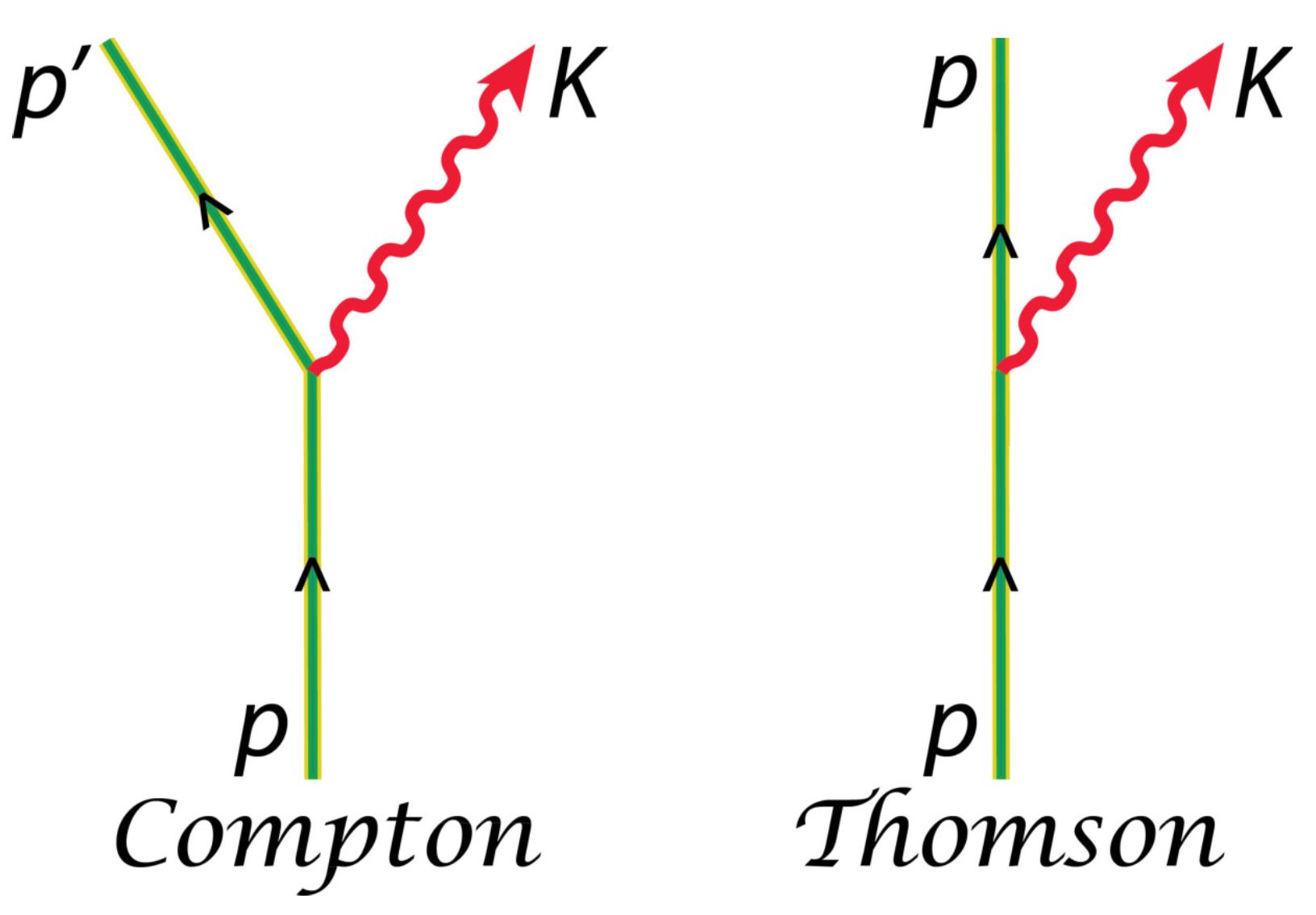
Let us start by considering the Feynman diagram for the Thomson scattering, shown in Figure 1 (right). While the wiggly line corresponds to the scattered radiation (four-momentum K), the straight line represents the electron in the laser field (four-momentum p). Contrary to Compton process, the particle does not change its momentum during the scattering (cf. Figure 1, left) as the quantum recoil effects are absent.

In Section 2.1, we calculate the electron trajectory (Equations (19) and (20)) and its “acceleration” with respect to the phase (Equations (21) and (22)) in an arbitrary electromagnetic field $\mathit{A}\left(\varphi \right)$. From now on, we assume that the particle travels with four-momentum p before the interaction with the laser pulse, defined by Equation (23). The angular-frequency energy distribution is determined by the Thomson formula [61]

$$\frac{{\mathrm{d}}^3{E}_{\mathrm{Th}}}{\mathrm{d}{\omega }_{\mathit{K}}{\mathrm{d}}^2{\mathsf{\Omega }}_{\mathit{K}}}=\frac{e^2}{4\pi {\epsilon }_{0}c}{\left|{\mathcal{A}}_{\mathrm{Th}}\right|}^2,$$

(40)

where ${\omega }_{\mathit{K}}$ is the frequency of the radiation scattered in the solid angle ${\mathrm{d}}^2{\mathsf{\Omega }}_{\mathit{K}}$, and ${\epsilon }_0$ is the electric permittivity of free space. The classical amplitude ${\mathcal{A}}_{\mathrm{Th}}$, calculated with respect to the phase $\varphi$, is given by [26,58]

$${\mathcal{A}}_{\mathrm{Th}}=\frac{1}{2\pi }{\int }_0^{2\pi }\mathsf{{\rm Y}}\left(\varphi \right)exp\left(\mathrm{i}\frac{{\omega }_{\mathit{K}}}{\omega }\varphi +\mathrm{i}\frac{{\omega }_{\mathit{K}}}{c}[\mathit{n}-{\mathit{n}}_{\mathit{K}}]·\mathit{x}\left(\varphi \right)\right)\mathrm{d}\varphi ,$$

(41)

with ${\mathit{n}}_{\mathit{K}}$ being the propagation direction of the emitted radiation, $\mathit{x}\left(\varphi \right)$ the trajectory of the electron and the function

$$\mathsf{{\rm Y}}\left(\varphi \right)=\frac{{\mathit{n}}_{\mathit{K}}\times [({\mathit{n}}_{\mathit{K}}-\mathit{\beta }\left(\varphi \right))\times {\mathit{\beta }}^{\prime }\left(\varphi \right)]}{{[1-{\mathit{n}}_{\mathit{K}}·\mathit{\beta }\left(\varphi \right)]}^2}$$

(42)

a partial amplitude. Here, we introduce the reduced velocity $\mathit{\beta }\left(t\right)=(1/c)\mathrm{d}\mathit{x}/\mathrm{d}t$, which, as a function of $\varphi$, is given by

$$\mathit{\beta }\left(\varphi \right)=\frac{{\mathit{x}}^{\prime }}{\frac{c}{\omega }+\mathit{n}·{\mathit{x}}^{\prime }}.$$

(43)

As before, the “prime” refers to the derivative with respect to the phase, i.e., ${\mathit{x}}^{\prime }\left(\varphi \right)=\mathrm{d}\mathit{x}/\mathrm{d}\varphi$. From Equation (43), it follows directly that

$${\mathit{\beta }}^{\prime }=\frac{{\mathit{x}}^{″}\left(\frac{c}{\omega }+\mathit{n}·{\mathit{x}}^{\prime }\right)-{\mathit{x}}^{\prime }(\mathit{n}·{\mathit{x}}^{″})}{{\left(\frac{c}{\omega }+\mathit{n}·{\mathit{x}}^{\prime }\right)}^2}.$$

(44)

Equations (40)–(44) show that the angular-frequency distribution is determined when the functions $\mathit{x}\left(\varphi \right)$, ${\mathit{x}}^{\prime }\left(\varphi \right)$, and ${\mathit{x}}^{″}\left(\varphi \right)$ are known. This is exactly the case, as they have been already presented in Section 2.1 (Equations (17)–(22)).

Sometimes, it is of interest to consider the polarization properties of the emitted radiation. For this reason, we introduce two vectors ${\mathit{\epsilon }}_{\mathit{K},\sigma }$, each one describing a polarization state $\sigma$ ($\sigma =1,2$). With this in mind, we define the scalar partial amplitude ${\mathsf{{\rm Y}}}_{\sigma }\left(\varphi \right)$ as ${\mathsf{{\rm Y}}}_{\sigma }\left(\varphi \right)={\mathit{\epsilon }}_{\mathit{K},\sigma }^{*}·\mathsf{{\rm Y}}\left(\varphi \right)$. Taking into account Equation (42), such quantity can be written in a relativistically invariant form as [58]

$${\mathsf{{\rm Y}}}_{\sigma }^{\mathrm{inv}}\left(\varphi \right)=\frac{{\mathsf{{\rm Y}}}_{\sigma }\left(\varphi \right)}{K^0}=\frac{({\epsilon }_{\mathit{K},\sigma }·x^{″})(K·x^{\prime })-({\epsilon }_{\mathit{K},\sigma }·x^{\prime })(K·x^{″})}{{(K·x^{\prime })}^2}$$

(45)

and the corresponding polarization-dependent Thomson amplitude is

$${\mathcal{A}}_{\mathrm{Th},\sigma }^{\mathrm{inv}}=\frac{1}{2\pi }{\int }_0^{2\pi }{\mathsf{{\rm Y}}}_{\sigma }^{\mathrm{inv}}\left(\varphi \right){\mathrm{e}}^{\mathrm{i}K·x\left(\varphi \right)}\mathrm{d}\varphi .$$

(46)

Note that, in the previous expressions, $x\equiv x\left(\varphi \right)$ is the four-position introduced in Section 2.1 and ${\epsilon }_{\mathit{K},\sigma }=(0,{\mathit{\epsilon }}_{\mathit{K},\sigma })$. Finally, the polarization-independent frequency distribution is given by

$$\frac{{\mathrm{d}}^3{E}_{\mathrm{Th}}}{\mathrm{d}{\omega }_{\mathit{K}}{\mathrm{d}}^2{\mathsf{\Omega }}_{\mathit{K}}}=\sum _{\sigma =1,2}\frac{{\mathrm{d}}^3{E}_{\mathrm{Th},\sigma }}{\mathrm{d}{\omega }_{\mathit{K}}{\mathrm{d}}^2{\mathsf{\Omega }}_{\mathit{K}}}\mathrm{and}\frac{{\mathrm{d}}^3{E}_{\mathrm{Th},\sigma }}{\mathrm{d}{\omega }_{\mathit{K}}{\mathrm{d}}^2{\mathsf{\Omega }}_{\mathit{K}}}=\alpha \frac{{\omega }_{\mathit{K}}^2}{c^2}{\left|{\mathcal{A}}_{\mathrm{Th},\sigma }^{\mathrm{inv}}\right|}^2,$$

(47)

with $\alpha =e^2/\left(4\pi {\epsilon }_{0}c\right)$ being the fine-structure constant. The invariant formulation of the Thomson scattering has many advantages. The most important one is that the probability amplitude can be calculated in an arbitrary reference frame before being Lorentz-transformed to any other frame of interest.

As is clear in the next section, Compton and Thomson formulas predict, in general, different frequencies of the emitted radiation. This is a consequence of the quantum recoil of the electron, present in Compton’s theory, and the energy-momentum conservation relations. There is also another fundamental difference between those two approaches: while the spin degrees of freedom are not accounted for in the classical evolution of the electron, they play a fundamental role in the Dirac theory. Those two main features lead to different classical and quantum predictions. However, as shown in Refs. [23,24,25,26], there exists a scaling law between the Compton and Thomson frequencies, for which the energy distributions are approximately equal. This is provided that spin effects do not play a role in the scattering dynamics and that the frequency of the emitted radiation is below a quantum cutoff.

4. Compton Scattering

The Compton process, which is the quantum counterpart of the Thomson scattering, was originally analyzed by A. H. Compton [19] in a 1923 paper. (For a detailed account of the events leading to Compton’s theory, we refer the reader to the historical review [18].) At the beginning of the 20th century, there was great controversy about the scattering of highly energetic radiation by solid materials [18]. Experiments carried out by D. C. H. Florance [62] and J. A. Gray [63,64] in the period 1910–1920 showed that the scattered X- or $\gamma$-rays present a softening (increase in wavelength) depending on the detection angle (see Ref. [18]). According to Thomson’s classical theory, the frequency of the emitted radiation should be, in principle, exactly equal to the frequency of the incident one. Hence, the observed softening was initially attributed to an angular separation of the wavelengths constituting the non-monochromatic incident beam by the action of the scatterer (see [18] and references therein). However, in 1921, Compton indicated that the secondary beam indeed presents “a real change in the character of the radiation” [65]. His explanation of this new character relied on the existence of an angular-dependent fluorescence mechanism induced by the incident beam; in such case, the emitted radiation could be softer than the incident one [18,65]. However, in 1923, the author discarded the fluorescence hypothesis and introduced the ideas of radiation quanta in scattering theory [19]. In contrast to the classical assumption that the energy of an electromagnetic wave is uniformly distributed over its wavefront, Compton suggested that the quantized unit “spends all of its energy and momentum upon some particular electron” [19]. By using the conservation relations, he concluded that not only would the electron experience a recoil, but also the scattered radiation should be characterized by a lower frequency. Compton calculated the difference in wavelength between the secondary and primary radiations as a function of the scattering angle. To corroborate his hypothesis, he measured the spectrum of molybdenum radiation and the spectrum of the rays scattered by a solid target (constant angle). The observed increase in wavelength was, indeed, very close to the one predicted by his theory. To demonstrate the angular-dependence of this increment, he determined experimentally the properties of scattered $\gamma$-rays at different angles. Again, the theoretical predictions were in good agreement with his observations. The author concluded that, in fact, scattering of electrons by electromagnetic radiation is of quantum nature. It is interesting to notice that Compton was not the only one working on the quantum description of electron scattering by light. It seems that Debye, independently, also derived the scattering formula [66]. However, the latter author agreed to give the credit of the discovery to Compton, due to the compelling theoretical and experimental evidence he presented. (For this and many more interesting historical remarks, we refer the reader to the book [18].) Finally, as it is argued there, the discovery of the Compton scattering was fundamental for the acceptance of the quantum theory of light.

Since the invention of lasers in 1960 [67,68], the Compton process has entered a new phase of research. With the availability of sources of coherent and strong radiation, new experimental and theoretical analyses were possible. Already in 1963, Nikishov and Ritus proposed the use of laser fields to analyze the radiation emitted by an electron in an electromagnetic plane wave, among other phenomena [69] (see also the recent articles [23,70] and references therein). In an article published the following year, the same authors made a distinction between two intensity-related regimes of the Compton process [71]: linear and non-linear Compton scattering (LCS and NLCS, respectively) (see Ref. [72] for more details); when light fields of relatively low intensity are considered, electron scattering by a single photon leads to the LCS; in contrast, at large intensities, the probability of interaction with multiple photons, and subsequent emission of a single one, becomes high. The last case corresponds to the NLCS [70,73]. Note, however, that most of the initial investigations concerning the linear and non-linear Compton processes were based on the assumption of a monochromatic plane wave of infinite duration, as pointed out in Refs. [70,73]. An important exception worth mentioning here is the early work of Neville and Rohrlich [74], who considered in 1971 the scattering of a spinless particle by a laser pulse of, in principle, finite duration [70]. Their treatment, based on the perturbation theory of the S-matrix formalism, was developed in a mixed framework where the particle experiences the influence of a strong, classical laser radiation while interacting with quantized modes of the electromagnetic field [74] (see also [23,73]). This approach is known as the Furry picture [23,74]. More recently, Narozhnyĭ and Fofanov [75] analyzed, theoretically, the spectral properties of Compton photons emitted in a head-on collision between relativistic electrons and finite-in-time, circularly-polarized laser pulses. The authors were motivated by the rapid advance in laser systems already observed in the 1990s, which allowed the production of very short and intense light pulses. Under such circumstances, the monochromatic plane wave approximation is no longer applicable and different theoretical tools had to be developed [75]. In 2009, Boca and Florescu [73] studied the NLCS induced by non-monochromatic laser pulses without the restrictive conditions imposed by Narozhnyĭ and Fofanov. This new treatment allowed the investigation of electron scattering by very short (few cycle) laser pulses, and the influence of the carrier-envelope phase on the emitted radiation [73].

In the remaining part of this section, we present an overview of the NLCS induced by short-in-time laser pulses in the plane-wave-fronted approximation. The treatment applied here is based on an extension of the original paper by Neville and Rohrlich [74] and the work of Boca and Florescu [73]. The full derivations and additional details can be found in Refs. [58,70].

Before presenting detailed derivations, let us give a general overview of the Compton scattering in the Furry picture by following the reasoning presented in [23,72]. Prior to scattering event, the electron is coupled to the strong, classical electromagnetic field $A\left(\varphi \right)$ defined in Equation (23), i.e., it is described by the Volkov solution in Equation (35) labeled by the initial momentum $\mathit{p}$ (before the interaction with the light pulse starts). The electromagnetic radiation induces an additional contribution to the momentum due to the oscillating motion in the field [23,72]. At certain time, such electron emits an extra non-laser photon and, subsequently, the particle is again described by the Volkov solution with asymptotic momentum ${\mathit{p}}^{\prime }$ (after the laser pulse has vanished). In Figure 1 (left), we present the Feynman diagram representing the Compton process described here. As stressed in Ref. [23], the straight lines are not associated with plane-wave free-electron states but correspond to the Volkov solutions Equation (35). The wiggly line represents the emitted radiation during the scattering event. Contrary to the Thomson process, the electron experiences a recoil upon the interaction with the laser photon, which explains its change in momentum. Furthermore, the emitted photon has a different frequency compared to the laser radiation. This is a consequence of the energy and momentum conservation relations, as already established by Compton [19].

Consider an electron with initial four-momentum p and spin polarization $\lambda$ interacting with a laser field. After scattering by the laser radiation, the particle is found with a final four-momentum $p^{\prime }$ and spin state ${\lambda }^{\prime }$; one photon of frequency ${\omega }_{\mathit{K}}=c{K}^0$ propagating along the direction ${\mathit{n}}_{\mathit{K}}$ is also emitted. Such photon is characterized by the wave and polarization four vectors, $K^{\mu }=(K^0,\mathit{K})=K^0(1,{\mathit{n}}_{\mathit{K}})$ and ${\epsilon }_{\mathit{K}\sigma }^{\mu }=(0,{\mathit{\epsilon }}_{\mathit{K}\sigma })$, respectively. Here, ${\mathit{\epsilon }}_{\mathit{K}\sigma }$ is a unit vector and $\sigma =1,2$ labels the polarization degrees of freedom. As it is for the primary radiation, the relations $K·K=0$ and $K·{\epsilon }_{\mathit{K}\sigma }=0$ also apply. Additionally, for two polarization states $\sigma ,{\sigma }^{\prime }$ we have that ${\epsilon }_{\mathit{K}\sigma }·{\epsilon }_{\mathit{K}{\sigma }^{\prime }}=-{\delta }_{\sigma ,{\sigma }^{\prime }}$. With the notation already introduced, we write the Compton probability amplitude for the scattering of electrons by the laser field as [70]

$${\mathcal{A}}_{\mathrm{C}}^{(++)}(\mathit{K}\sigma ;{\mathit{p}}^{\prime }{\lambda }^{\prime };\mathit{p}\lambda )=-\mathrm{i}e\int {\mathrm{d}}^{4}x{\left[j_{{\mathit{p}}^{\prime }{\lambda }^{\prime },\mathit{p}\lambda }^{(++)}\right]}^{\mu }{\left[A_{\mathit{K}\sigma }^{(-)}\left(x\right)\right]}_{\mu }.$$

(48)

Here, $j_{{\mathit{p}}^{\prime }{\lambda }^{\prime },\mathit{p}\lambda }^{(++)}$ is the four-component probability current for electrons ($\beta =+$) defined in Equation (39) and the term $A_{\mathit{K}\sigma }^{(-)}\left(x\right)$ is given by

$$A_{\mathit{K}\sigma }^{(-)}\left(x\right)=\sqrt{\frac{2\pi c\alpha }{e^2{\omega }_{\mathit{K}}V}}{\mathrm{e}}^{\mathrm{i}K·x}{\epsilon }_{\mathit{K}\sigma }^{*}.$$

(49)

Taking into account the analytical expressions of the Volkov solution in Equation (35) for the finite laser pulse in Equation (23), we write the probability amplitude for Compton scattering in Equation (48) in the Furry picture as [70]

$$\begin{array}{cc}\hfill {\mathcal{A}}_{\mathrm{C}}^{(++)}(\mathit{K}\sigma ;{\mathit{p}}^{\prime }{\lambda }^{\prime };\mathit{p}\lambda )=& \mathcal{A}({\omega }_{\mathit{K}},p_0,p_0^{\prime })\int {\mathrm{d}}^{4}xexp\left(-\mathrm{i}[S_p^{(+)}\left(x\right)-S_{p^{\prime }}^{(+)}\left(x\right)-K·x]\right)\hfill \\ \hfill \times & {\overline{u}}_{{\mathit{p}}^{\prime }{\lambda }^{\prime }}^{(+)}\left(1+\frac{e\cancel{A}\cancel{k}}{2p^{\prime }·k}\right){\epsilon }_{\mathit{K}\sigma }^{*}\left(1-\frac{e\cancel{A}\cancel{k}}{2p·k}\right)u_{\mathit{p}\lambda }^{(+)}.\hfill \end{array}$$

(50)

For simplicity, we introduce the amplitude prefactor ${\mathcal{A}}_0({\omega }_{\mathit{K}},p_0^{\prime },p_0)$, given by

$${\mathcal{A}}_0({\omega }_{\mathit{K}},p_0^{\prime },p_0)=\mathrm{i}\sqrt{\frac{2\pi \alpha m_{\mathrm{e}}^2{c}^3}{p_0^{\prime }{p}_0{\omega }_{\mathit{K}}{V}^3}}.$$

(51)

Up to now, the laser four-vector potential has been presented in the general way $A(k·x)=A\left(\varphi \right)$. In the following, we express the Compton amplitude in Equation (51) in terms of the shape functions $f_1(k·x)$ and $f_2(k·x)$ introduced in Equation (23). Namely, we write

$$\begin{array}{cc}\hfill {\mathcal{A}}_{\mathrm{C}}^{(++)}& (\mathit{K}\sigma ;{\mathit{p}}^{\prime }{\lambda }^{\prime };\mathit{p}\lambda )=\mathcal{A}({\omega }_{\mathit{K}},p_0,p_0^{\prime })\int {\mathrm{d}}^{4}xexp\left(-\mathrm{i}[S_p^{(+)}\left(x\right)-S_{p^{\prime }}^{(+)}\left(x\right)-K·x]\right)\hfill \\ \hfill \times & \left[{\overline{u}}_{{\mathit{p}}^{\prime }{\lambda }^{\prime }}^{(+)}\left(1-\frac{\mu m_{\mathrm{e}}c}{2p^{\prime }·k}[f_1(k·x){\cancel{\epsilon }}_1+f_2(k·x){\cancel{\epsilon }}_2]\cancel{k}\right){\cancel{\epsilon }}_{\mathit{K}\sigma }^{*}\left(1+\frac{\mu m_{\mathrm{e}}c}{2p·k}[f_1(k·x){\cancel{\epsilon }}_1+f_2(k·x){\cancel{\epsilon }}_2]\cancel{k}\right)u_{\mathit{p}\lambda }^{(+)}\right].\hfill \end{array}$$

(52)

Note that in the integrand, besides the exponential factor, the only functions depending on x are $f_1(k·x)$ and $f_2(k·x)$. Hence, by following the derivations in [70], Equation (52) can be written as a sum of integrals of the type

$$C^{(n,m)}=\int {\mathrm{d}}^{4}x{\left[f_1(k·x)\right]}^n{\left[f_2(k·x)\right]}^{m}exp\left(-\mathrm{i}[S_p^{(+)}\left(x\right)-S_{p^{\prime }}^{(+)}\left(x\right)-K·x]\right),$$

(53)

where $n,m=0,1,2$. For our further purposes, we express the exponent in Equation (53) in the following way,

$$\begin{array}{cc}\hfill S_p^{(+)}\left(x\right)-S_{p^{\prime }}^{(+)}\left(x\right)-& K·x=(p-p^{\prime }-K)·x+{\int }_0^{k·x}\mathrm{d}\phi (-\mu m_{\mathrm{e}}c\left[\frac{p·{\epsilon }_1}{p·k}-\frac{p^{\prime }·{\epsilon }_1}{p^{\prime }·k}\right]f_1\left(\phi \right)\hfill \\ \hfill -& \mu m_{\mathrm{e}}c\left[\frac{p·{\epsilon }_2}{p·k}-\frac{p^{\prime }·{\epsilon }_2}{p^{\prime }·k}\right]f_2\left(\phi \right)+\frac{{\left(\mu m_{\mathrm{e}}c\right)}^2}{2}\left[\frac{1}{p·k}-\frac{1}{p^{\prime }·k}\right][f_1^2\left(\phi \right)+f_2^2\left(\phi \right)])\hfill \end{array}$$

(54)

$$\begin{array}{cc}\hfill \equiv & Q·x+{\int }_0^{k·x}\mathrm{d}\phi \left(a_1{f}_1\left(\phi \right)+a_2{f}_2\left(\phi \right)+a_{1,2}[f_1^2\left(\phi \right)+f_2^2\left(\phi \right)]\right).\hfill \end{array}$$

(55)

Equations (54) and (55) implicitly define the factors $a_1$, $a_2$, and $a_{1,2}$, together with the four vector Q. All of them are independent of x. This is useful for the application of the Boca–Florescu transformation [70,73] (see below).

At this point, let us separate the integrals $C^{(n,m)}$ into two groups. The first group, characterized by n and m such that $n\ne 0$ or $m\ne 0$, contains vanishing integrands outside the interval $k·x\in ]0,2\pi [$. On the other hand, as noted by Boca and Florescu [73], the term corresponding to $C^{(0,0)}$ behaves differently and requires a separate treatment. We start by considering this case first.

As shown above, to calculate the Compton probability amplitude, it is necessary to perform all integrals $C^{(n,m)}$ for $n,m=0,1,2$. However, the different character of $C^{(0,0)}$ complicates the situation. It would be useful to transform this integral such that it could be expressed in a similar way as the other $C^{(n,m)}$. In fact, this can be done by means of the Boca–Florescu transformation (BFT) [73] (see also Appendix B in Ref. [70]). To this end, we write $C^{(0,0)}$ as follows,

$$C^{(0,0)}=\int {\mathrm{d}}^{4}xexp\left[-\mathrm{i}{\int }_0^{k·x}\mathrm{d}\phi h\left(\phi \right)-\mathrm{i}Q·x\right],$$

(56)

where $h\left(\phi \right)=a_1{f}_1\left(\phi \right)+a_2{f}_2\left(\phi \right)+a_{1,2}[f_1^2\left(\phi \right)+f_2^2\left(\phi \right)]$ is an integrable function, which vanishes at $\phi <0$ and $\phi >2\pi$. According to the BFT (see Ref. [70] for details), Equation (56) can be rewritten as

$$\begin{array}{cc}\hfill C^{(0,0)}=& -\frac{k^0}{Q^0}\int {\mathrm{d}}^{4}xh(k·x)exp\left[-\mathrm{i}{\int }_0^{k·x}\mathrm{d}\phi h\left(\phi \right)-\mathrm{i}Q·x\right]\hfill \\ \hfill =& \int {\mathrm{d}}^{4}x\left({\tilde{a}}_1{f}_1(k·x)+{\tilde{a}}_2{f}_2(k·x)+{\tilde{a}}_{1,2}[f_1^2(k·x)+f_2^2(k·x)]\right)exp\left[-\mathrm{i}{\int }_0^{k·x}\mathrm{d}\phi h\left(\phi \right)-\mathrm{i}Q·x\right].\hfill \end{array}$$

(57)

Here, $\tilde{a}=-k^{0}a/Q^0$ for a being $a_1$, $a_2$ or $a_{1,2}$ and $Q^0\ne 0$, which is always satisfied in the process under consideration [70]. Hence, from Equation (57) and the definition in Equation (53), we can express $C^{(0,0)}$ in terms of the other integrals, namely

$$C^{(0,0)}={\tilde{a}}_1{C}^{(1,0)}+{\tilde{a}}_2{C}^{(0,1)}+{\tilde{a}}_{1,2}[C^{(2,0)}+C^{(0,2)}].$$

(58)

The BFT has then reduced the problem to the calculation of the remaining $C^{(n,m)}$. We now consider this case. First, we introduce the so-called laser-dressed four-momentum $\overline{p}$ given by

$$\begin{array}{cc}\hfill \overline{p}=p-& \frac{m_{\mathrm{e}}c\mu }{p·k}({\epsilon }_1·p\langle f_1\rangle +{\epsilon }_2·p\langle f_2\rangle )k+\frac{{\left(m_{\mathrm{e}}c\mu \right)}^2}{2p·k}(\langle f_1^2\rangle +\langle f_2^2\rangle )k,\hfill \end{array}$$

(59)

where the angular brackets $\langle F\rangle$ denote the average of the function $F\left(\varphi \right)$ over the duration of the pulse. This means that, if $F\left(\varphi \right)$ is integrable and vanishes outside the interval $0⩽\varphi ⩽2\pi$, then

$$\langle F\rangle =\frac{1}{2\pi }{\int }_0^{2\pi }\mathrm{d}\varphi F\left(\varphi \right).$$

(60)

Note that the definition in Equation (59), which comes from the analytical form of the Volkov solution in Equation (35), is arbitrary [27,76]. Namely, the probability amplitude of scattering in the laser field depends on the four-current in Equation (39), thus the measurable quantity is always the difference $\overline{p}-{\overline{p}}^{\prime }$. In other words, all physical quantities remain unchanged by adding an extra term, independent of p and vanishing in the absence of the laser pulse, to the dressed four-momentum. Furthermore, it is noteworthy that $\overline{p}$, as presented in Equation (59), is only on the mass shell if $\langle f_1\rangle =\langle f_2\rangle =0$, which is not always the case for a single and short laser pulse. This problem can be solved by introducing the transformation (see Ref. [27])

$$\overline{p}\to \overline{p}+\mu m_{\mathrm{e}}c(\langle f_1\rangle {\epsilon }_1+\langle f_2\rangle {\epsilon }_2).$$

(61)

In this particular case, we obtain that $\overline{p}·\overline{p}={\overline{m}}_{\mathrm{e}}^2{c}^2$, where ${\overline{m}}_{\mathrm{e}}$ is the effective mass of the electron, given by

$${\overline{m}}_{\mathrm{e}}^2=m_{\mathrm{e}}^2\left(1+\frac{2U_p}{m_{\mathrm{e}}{c}^2}\right)$$

(62)

and $U_p$ is the ponderomotive energy of the electron in the laser pulse, i.e.,

$$U_p=\frac{{\mu }^2{m}_{\mathrm{e}}{c}^2}{2}(\langle f_1^2\rangle -{\langle f_1\rangle }^2+\langle f_2^2\rangle -{\langle f_2\rangle }^2),$$

(63)

(see also the analysis about the mass shift presented by Harvey et al. in Ref. [77] and the discussion in [27]). However, as our main concern is the calculation of the probability amplitude in Compton scattering, we remain with the definition in Equation (59). In doing so, we recast the exponent in Equation (53) in terms of a function $G(k·x)$, which depends on x only through the phase of the laser pulse. In terms of the parameters $a_1$, $a_2$ and $a_{1,2}$, introduced in Equation (55), this function is given by

$$\begin{array}{cc}\hfill G(k·x)=& {\int }_0^{k·x}\mathrm{d}\phi \left[a_1(f_1\left(\phi \right)-\langle f_1\rangle )+a_2(f_2\left(\phi \right)-\langle f_2\rangle )+a_{1,2}(f_1^2\left(\phi \right)+f_2^2\left(\phi \right)-\langle f_1^2\rangle -\langle f_2^2\rangle )\right]\hfill \end{array}$$

(64)

such that

$$S_p^{(+)}\left(x\right)-S_{p^{\prime }}^{(+)}\left(x\right)-K·x=(\overline{p}-{\overline{p}}^{\prime }-K)·x+G(k·x).$$

(65)

At this point, the functions $C^{(n,m)}$ in Equation (53) can be obtained with the introduction of the following Fourier decomposition,

$${\left[f_1(k·x)\right]}^n{\left[f_2(k·x)\right]}^m{\mathrm{e}}^{-\mathrm{i}G(k·x)}=\sum _{N=-\infty }^{\infty }{G}_N^{\left(n,m\right)}{\mathrm{e}}^{-\mathrm{i}Nk·x},0⩽k·x⩽2\pi .$$

(66)

This leads to the expression

$$\begin{array}{cc}\hfill C^{(n,m)}=& \sum _{N=-\infty }^{\infty }{G}_N^{\left(n,m\right)}\int {\mathrm{d}}^{4}xexp\left(-\mathrm{i}[\overline{p}-{\overline{p}}^{\prime }+Nk-K]·x\right)\equiv \sum _{N=-\infty }^{\infty }{G}_N^{\left(n,m\right)}\int {\mathrm{d}}^{4}x{\mathrm{e}}^{-\mathrm{i}{P}_N·x},\hfill \end{array}$$

(67)

where we have introduced the four-vector $P_N=\overline{p}-{\overline{p}}^{\prime }+Nk-K$. Note that the integration measure ${\mathrm{d}}^{4}x$ is restricted to such x for which $0⩽k·x⩽2\pi$. For this reason, it is convenient to introduce the so-called light-cone coordinates (see, e.g., [70,78,79]), defined with respect to the laser pulse propagation direction $\mathit{n}$. The four-position, in this coordinate system, is represented as

$$x^{\parallel }=\mathit{n}·\mathit{x},{\mathit{x}}^{\perp }=\mathit{x}-x^{\parallel }\mathit{n},x^{-}=x^0-x^{\parallel },x^{+}=(x^0+x^{\parallel })/2,$$

(68)

the integration measure takes the form ${\mathrm{d}}^{4}x=\mathrm{d}{x}^{+}\mathrm{d}{x}^{-}{\mathrm{d}}^2{x}^{\perp }$ and, in particular, $P_N·x=P_N^{+}{x}^{-}+P_N^{-}{x}^{+}-{\mathit{P}}_N^{\perp }·{\mathit{x}}^{\perp }$. The phase of the laser field is now given by $\varphi =k·x=k^0{x}^{-}$. Thus, due to the finite duration of the pulse, the integration variable $x^{-}$ changes from 0 to $2\pi /k^0$. With this in mind, we write $C^{(n,m)}$ in Equation (67) as

$$\begin{array}{cc}\hfill C^{(n,m)}=& \sum _{N=-\infty }^{\infty }{G}_N^{\left(n,m\right)}\int \mathrm{d}{x}^{+}{\mathrm{d}}^2{x}^{\perp }{\int }_0^{2\pi /k^0}\mathrm{d}{x}^{-}exp\left[-\mathrm{i}(P_N^{+}{x}^{-}+P_N^{-}{x}^{+}-{\mathit{P}}_N^{\perp }·{\mathit{x}}^{\perp })\right]\hfill \\ \hfill =& {\left(2\pi \right)}^3\sum _{N=-\infty }^{\infty }{G}_N^{\left(n,m\right)}{\delta }^{\left(1\right)}\left(P_N^{-}\right){\delta }^{\left(2\right)}\left({\mathit{P}}_N^{\perp }\right)\left[\frac{1-{\mathrm{e}}^{-2\pi \mathrm{i}{P}_N^{+}/k^0}}{\mathrm{i}{P}_N^{+}}\right].\hfill \end{array}$$

(69)

Therefore, the Compton probability amplitude in Equation (52) takes the form

$${\mathcal{A}}_{\mathrm{C}}^{(++)}(\mathit{K}\sigma ;{\mathit{p}}^{\prime }{\lambda }^{\prime };\mathit{p}\lambda )={\left(2\pi \right)}^3\mathcal{A}({\omega }_{\mathit{K}},p_0,p_0^{\prime })\sum _{N=-\infty }^{\infty }{\delta }^{\left(1\right)}\left(P_N^{-}\right){\delta }^{\left(2\right)}\left({\mathit{P}}_N^{\perp }\right)\frac{1-{\mathrm{e}}^{-2\pi \mathrm{i}{P}_N^{+}/k^0}}{\mathrm{i}{P}_N^{+}}{D}_N,$$

(70)

where

$$\begin{array}{c}{D}_N={\overline{u}}_{{\mathit{p}}^{\prime }{\lambda }^{\prime }}^{(+)}\{{\cancel{\epsilon }}_{\mathit{K}\sigma }^{*}{\tilde{G}}_N^{(0,0)}+\frac{\mu m_{\mathrm{e}}c}{2}\left[\left(\frac{{\cancel{\epsilon }}_{\mathit{K}\sigma }^{*}{\cancel{\epsilon }}_{1}k}{p·k}-\frac{{\cancel{\epsilon }}_1\cancel{k}{\cancel{\epsilon }}_{\mathit{K}\sigma }^{*}}{p^{\prime }·k}\right)G_N^{(1,0)}+\left(\frac{{\cancel{\epsilon }}_{\mathit{K}\sigma }^{*}{\cancel{\epsilon }}_2\cancel{k}}{p·k}-\frac{{\cancel{\epsilon }}_2\cancel{k}{\cancel{\epsilon }}_{\mathit{K}\sigma }^{*}}{p^{\prime }·k}\right)G_N^{(0,1)}\right]\hfill \\ -\frac{{\left(\mu m_{\mathrm{e}}c\right)}^2}{4(p·k)(p^{\prime }·k)}[{\cancel{\epsilon }}_1\cancel{k}{\cancel{\epsilon }}_{\mathit{K}\sigma }^{*}{\cancel{\epsilon }}_1\cancel{k}{G}_N^{(2,0)}+{\cancel{\epsilon }}_2\cancel{k}{\cancel{\epsilon }}_{\mathit{K}\sigma }^{*}{\cancel{\epsilon }}_2\cancel{k}{G}_N^{(0,2)}+({\cancel{\epsilon }}_1\cancel{k}{\cancel{\epsilon }}_{\mathit{K}\sigma }^{*}{\cancel{\epsilon }}_2\cancel{k}+{\cancel{\epsilon }}_2\cancel{k}{\cancel{\epsilon }}_{\mathit{K}\sigma }^{*}{\cancel{\epsilon }}_1\cancel{k})G_N^{(1,1)}]\}{u}_{\mathit{p}\lambda }^{(+)}.\hfill \end{array}$$

(71)

To account for the $C^{(0,0)}$ integral, we introduce the modified Fourier coefficient

$${\tilde{G}}^{(0,0)}={\tilde{a}}_1{G}_N^{(1,0)}+{\tilde{a}}_2{G}_N^{(0,1)}+{\tilde{a}}_{1,2}[G_N^{(2,0)}+G_N^{(0,2)}],$$

(72)

which comes from our analysis of the BFT (see Equation (58)). Note that each term in the sum in Equation (70) constitutes an individual non-linear contribution to the overall probability amplitude. For the case of a monochromatic laser field, the integer N is interpreted as the number of photons absorbed in the scattering process [70]. In addition, from the delta functions in this equation, the definition of $P_N$ and the light-cone coordinates, the conservation relations can be identified. In doing so, we find (see Ref. [27]),

$$(\overline{p}-{\overline{p}}^{\prime }-K)·n=0,\mathrm{and}{\overline{\mathit{p}}}^{\perp }-{\overline{\mathit{p}}}^{\prime \perp }-{\mathit{K}}^{\perp }=\mathbf{0}.$$

(73)

This set of equations, together with other considerations, can be used to determine the final electron momenta for well-defined initial conditions by measuring the properties of the emitted radiation.

Once the probability amplitude of scattering in Equation (70) is obtained, it is possible to calculate the energy spectra of Compton photons for a given initial electron spin state $\lambda$ and final photon polarization $\sigma$. In doing so, one arrives at the following expression (see Ref. [70] for more details as well as Refs. [80,81]),

$$\frac{{\mathrm{d}}^3{E}_{\mathrm{C}}(\mathit{K}\sigma ;\mathit{p}\lambda )}{\mathrm{d}{\omega }_{\mathit{K}}{\mathrm{d}}^2{\mathsf{\Omega }}_{\mathit{K}}}=\sum _{{\lambda }^{\prime }=\pm }\frac{\alpha m_{\mathrm{e}}^2{c}^2{\left(K^0\right)}^2}{{\left(2\pi \right)}^2(k·p)(k·p^{\prime })}|\sum _N{D}_N\frac{1-{\mathrm{e}}^{-2\pi \mathrm{i}{P}_N^0/k^0}}{P_N^0/k^0}{|}^2,$$

(74)

where $D_N$ is given by Equation (71). Here, ${\mathsf{\Omega }}_{\mathit{K}}$ is the solid angle at which the Compton photon of frequency ${\omega }_{\mathit{K}}$ is detected. The spin- and polarization-independent probability distribution is obtained from Equation (74) by summing over the final polarization states while averaging with respect to the initial spin degrees of freedom,

$$\frac{{\mathrm{d}}^3{E}_{\mathrm{C}}}{\mathrm{d}{\omega }_{\mathit{K}}{\mathrm{d}}^2{\mathsf{\Omega }}_{\mathit{K}}}=\sum _{\sigma =1,2}\frac{{\mathrm{d}}^3{E}_{\mathrm{C},\sigma }}{\mathrm{d}{\omega }_{\mathit{K}}{\mathrm{d}}^2{\mathsf{\Omega }}_{\mathit{K}}}\mathrm{and}\frac{{\mathrm{d}}^3{E}_{\mathrm{C},\sigma }}{\mathrm{d}{\omega }_{\mathit{K}}{\mathrm{d}}^2{\mathsf{\Omega }}_{\mathit{K}}}=\frac{1}{2}\sum _{\lambda =\pm }\frac{{\mathrm{d}}^3{E}_{\mathrm{C}}(\mathit{K}\sigma ;\mathit{p}\lambda )}{\mathrm{d}{\omega }_{\mathit{K}}{\mathrm{d}}^2{\mathsf{\Omega }}_{\mathit{K}}}.$$

(75)

It is clear that the quantum calculations, from the theoretical and numerical point of view, require a considerably larger effort as compared to the classical ones. For this reason, it is of interest to analyze the Compton and Thomson polarization-dependent angular-frequency distributions [Equations (47) and (75)] in order to determine the parameters for which they coincide. Heinzl, Seipt, and Kämpfer [23] (see also Refs. [24,25]) found a scaling law between the Thomson and Compton frequencies (now denoted as ${\omega }_{\mathit{K}}^{\mathrm{Th}}$ and ${\omega }_{\mathit{K}}$, respectively) which relate both spectral responses, provided that the driving fields are monochromatic or are characterized by slowly-varying envelopes. This was later generalized by Krajewska and Kamiński [26] for the case of arbitrary ultrashort laser pulses. According to them, such scaling law is defined by the relation

$${\omega }_{\mathit{K}}^{\mathrm{Th}}=\frac{{\omega }_{\mathit{K}}}{1-\frac{{\omega }_{\mathit{K}}}{{\omega }_{\mathrm{cut}}}},$$

(76)

where

$${\omega }_{\mathrm{cut}}=\frac{1}{\hslash }\frac{cp·n}{n·n_{\mathit{K}}}$$

(77)

is the so-called cutoff, i.e., the maximum photon frequency emitted in Compton scattering. (Here, we have exceptionally restored the reduced Planck constant, ℏ, to underline the quantum nature of ${\omega }_{\mathrm{cut}}$.) Furthermore, the authors found that the polarization-dependent classical and quantum spectra are related by the formula

$$\frac{{\mathrm{d}}^3{E}_{\mathrm{C},\sigma }}{\mathrm{d}{\omega }_{\mathit{K}}{\mathrm{d}}^2{\mathsf{\Omega }}_{\mathit{K}}}=\gamma ({\omega }_{\mathit{K}},{\mathsf{\Omega }}_{\mathit{K}})\frac{{\mathrm{d}}^3{E}_{\mathrm{Th},\sigma }}{\mathrm{d}{\omega }_{\mathit{K}}^{\mathrm{Th}}{\mathrm{d}}^2{\mathsf{\Omega }}_{\mathit{K}}}{|}_{{\omega }_{\mathit{K}}^{\mathrm{Th}}=\frac{{\omega }_{\mathit{K}}}{1-{\omega }_{\mathit{K}}/{\omega }_{\mathrm{cut}}}},$$

(78)

where $\gamma ({\omega }_{\mathit{K}},{\mathsf{\Omega }}_{\mathit{K}})$ is a smooth and slowly varying function. This means that both distributions coincide, up to a multiplicative factor, when the Thomson frequency is rescaled according to Equation (76). However, such approximation is valid provided that the spin is conserved during the scattering (this is actually expected, as classical particles do not have spin degrees of freedom) and that the frequency of the emitted radiation is smaller than ${\omega }_{\mathrm{cut}}$. Furthermore, only when this frequency is much smaller than the cutoff, the Thomson and Compton spectra become identical, i.e., the corrections in the scaling law are negligible. In this sense, the scaling formula augmented considerably the previously-known range of validity of the Thomson process.

At this point, we make some comments about the Klein–Nishina (KN) formula and its generalization to ultrashort laser pulses. As mentioned above, the integer number N, which appears in the Compton probability amplitude in Equation (70), defines the number of laser photons absorbed during scattering, provided that the driving field approximates a monochromatic plane wave. In such case, the KN formula takes the form

$${\omega }_{\mathit{K},N}=\frac{N\omega }{\frac{p·n_{\mathit{K}}}{p·n}+\frac{U_p^{\mathrm{m}.}}{c}\frac{n·n_{\mathit{K}}}{p·n}+\frac{N\omega }{{\omega }_{\mathrm{cut}}}}.$$

(79)

It determines the frequency ${\omega }_{\mathit{K},N}$ of the emitted radiation in the direction ${\mathit{n}}_{\mathit{K}}$ [i.e., $n_{\mathit{K}}=(1,{\mathit{n}}_{\mathit{K}})$], after the electron absorbed N quanta. Here, $U_p^{\mathrm{m}.}={\mu }^2{\left(m_{\mathrm{e}}{c}^2\right)}^2/(4cp·n)$ is the ponderomotive energy of the electron in the monochromatic field. On the other hand, two effects can take place when the driving field lasts for a very short time [27]: first, due to the uncertainty principle together with multiple incoherent contributions to the total probability amplitude, the individual Compton peaks are broadened and cannot be properly resolved. Second, the KN formula [Equation (79)] is no longer applicable, as it requires laser fields for which $\langle f_1\rangle =\langle f_2\rangle \approx 0$ (this is not the case for finite-in-time pulses). The first problem can be addressed by using trains consisting of $N_{\mathrm{rep}}$ pulses with $N_{\mathrm{osc}}$ field oscillations within each individual envelope. This causes a “coherent enhancement of the Compton amplitude”, leading to an increment of the signal by the factor $N_{\mathrm{rep}}^2$ in the frequency spectra [27]. The second problem requires a modification to Equation (79), which is the so-called generalized Klein–Nishina formula (GKN) [27]. The latter accounts for the finite time duration of each pulse from a train, and can be written as

$${\omega }_{\mathit{K},N}^{\mathrm{GKN}}=\frac{(N/N_{\mathrm{osc}}){\omega }_{\mathrm{L}}}{\frac{p·n_{\mathit{K}}}{p·n}+\frac{\nu n·n_{\mathit{K}}+\mu m_{\mathrm{e}}c(\langle f_1\rangle q_1+\langle f_2\rangle q_2)}{{(p·n)}^2}+\frac{(N/N_{\mathrm{osc}}){\omega }_L}{{\omega }_{\mathrm{cut}}}},$$

(80)

where the scalar quantities $q_i$ ($i=1,2$) and $\nu$ are defined as

$$q_i=(p·n)(n_{\mathit{K}}·{\epsilon }_i)-(p·{\epsilon }_i)(n·n_{\mathit{K}})\mathrm{and}\nu =\frac{{\mu }^2{\left(m_{\mathrm{e}}c\right)}^2}{2}(\langle f_1^2\rangle +\langle f_2^2\rangle )$$

(81)

and the frequency of the field is ${\omega }_{\mathrm{L}}=N_{\mathrm{rep}}{N}_{\mathrm{osc}}\omega$. Furthermore, as shown in [27], a detailed analysis of such spectra can be used to determine important parameters of the driving field, when measured at different collision geometries. Hence, the GKN formula could provide a novel diagnostics tool for intense and short laser pulses.

In closing this section, we mention the most important experimental evidence of non-linear quantum electrodynamics, the SLAC experiment [82]. In this experiment, electron–positron pair creation was observed during the collision of highly energetic electrons and intense laser fields. It is agreed that such process happens in two steps: first, a highly energetic photon is produced during Compton back-scattering; second, such photon interacts with multiple laser photons in the non-linear Breit–Wheeler process producing the pairs (see Refs. [82,83] and references therein). However, it is worth mentioning that another single-step phenomenon, the trident process (which involves the collision of fast electrons with photons leading to pair production), can also occur (see Ref. [83]).

5. Møller Scattering

Only few years after Dirac published his equation, the Danish physicist Christian Møller successfully treated the electron-electron scattering from a relativistic and quantum point of view [15,16]. His work, originally oriented towards the problem of the stopping process (the mechanisms for which relativistic electrons are stopped by matter), led to the celebrated Møller formula, which determines the scattering cross-section for the collision of two relativistic electrons (see the historical reviews [12,13]). As mentioned in those reviews, this problem was already considered by Bethe from a non-relativistic perspective. Formally, he demonstrated that the impact of two charged particles can be described in terms of an effective electrostatic potential consistent with an effective charge distribution. The scattering problem is then reduced to the Coulomb interaction between a moving particle and the apparent effective charge created by the other one. As discussed in [13], Møller’s great achievement was the generalization of Bethe’s ideas to the relativistic case. The introduction of a retarded potential with the effective charge and current distributions, treated in accordance to the Bohr’s correspondence principle, was considered in [15] (see Refs. [12,13]).

After the invention of the laser, a renewed attention was given to light-assisted scattering processes. Already in 1967, V. P. Oleĭnik analyzed the Møller scattering in the presence of an infinite, monochromatic, and circularly polarized plane wave [84,85]. By calculating the effective cross-section, the author demonstrated that, for certain parameters of the electrons momenta and electromagnetic radiation, strong resonances may occur. Furthermore, he showed that the electron in the laser field behaves similarly to a “quasiparticle” characterized by an infinite number of discrete energy states with finite lifetimes. Hence, for appropriate parameters of the interaction, resonance effects should be observed. Additionally, Oleĭnik showed that the effective interaction between the two electrons can become attractive due to their interaction with the electromagnetic radiation. More than ten years later, Bös et al. [86,87] reanalyzed the problem of resonances in Møller scattering in the same type of laser fields (namely, in circularly-polarized monochromatic plane waves) and for non-relativistic electrons with opposite initial momenta. As they have shown, the presence of the electromagnetic radiation modifies the field-free process in three fundamental ways: (i) both electrons can absorb or radiate an integer number of laser photons; (ii) their effective masses are modified; and (iii) light-induced scattering resonances can, in fact, appear. As a consequence of (i) and (ii), the conservation relations turn out to be different in the presence of the light field. This leads to a discrete and intensity-dependent energy spectra of scattered electrons. In another paper, Bergou, Varró and Fedorov [88] also analyzed the laser-assisted Møller scattering from a non-relativistic point of view. It was demonstrated there that the dipole approximation can be used to transform the Schrödinger equation into two different equations, one accounting for the interaction with the laser field and the other one for the charge repulsion. Hence, they concluded that the laser effects in the scattering process require a treatment beyond such approximation. In doing so, the authors analyzed the intensity-dependent momentum and energy conservation relations in the non-relativistic case and the resonance phenomena for a screened Coulomb potential. They also corroborated that resonances can be related to bound(-like) states caused by the effective attraction experienced by the particles. Few years later, Kazantsev and Sokolov [89] (see also Ref. [90]) studied classically the dynamics of two electrons in laser fields. They found that for very intense radiation the effective potential can, in fact, be attractive and may lead to the aforementioned bound states (see also the review [91]). In Ref. [92], Fedorov and Roshchupkin examined the influence of the laser field on interference effects far from resonances. Those interferences arise from the exchange and direct contributions to the Møller-assisted process and, as the authors showed, they can be suppressed for certain parameters of the light-matter interaction.

Already in the 1990s, Denisenko and Roshchupkin [93] examined the Møller scattering in more complex laser fields under non-resonant conditions. In particular, they considered bi-chromatic linearly- or circularly-polarized plane wave fields and determined their influence on the laser-assisted process (see also [94]). In a series of papers, Starodub, Roshchupkin and co-authors [91,95,96,97,98] studied the effective forces experienced by two electrons in the presence of light pulses. The influence of laser fields composed by counter-propagating, co-propagating or perpendicularly-propagating pulses of radiation was also considered. Their treatment was based on the solution of the classical equations of motion governing the dynamics of non-relativistic particles in the field. The authors determined the pulse parameters for which the electron-electron (e-e) interaction becomes attractive or for which the so-called anomalous repulsion can take place [98]. For the laser-assisted Møller process from a quantum electrodynamics point of view, Padusenko and Roshchupkin [99] calculated the scattering cross-section under resonant conditions for light pulses of relatively long duration. This mechanism was also generalized there for the case of two-lepton scattering in an electromagnetic wave. In addition, in Ref. [100], Lebed’ et al. considered the resonance effects in ultrarelativistic e-e collisions in laser pulses at small scattering angles. In the same reference, the influence of the light field polarization properties on the scattering cross-section received attention. For a detailed analysis of resonant and non-resonant Møller-like scattering (and other processes) in long-in-time laser pulses, we refer the reader to the reviews [101,102], and references therein.

In 2004, Panek et al. [103] studied the Møller scattering in linearly-polarized laser fields of relativistic intensities (the ponderomotive energy of the electron in the plane wave is similar or larger than its rest energy). They determined the circumstances for which resonances can take place. The authors showed that, under non-resonant conditions and for certain parameters of the e-e collision, the resulting scattering cross-sections are minimal. In the terminology coined by them, there exist “dark angular windows” when the scattering angles are sufficiently small [103]. Møller scattering in super intense laser fields was also presented in the review article [28], together with other fundamental phenomena in strong-field quantum electrodynamics. In the following, it is our aim to summarize some of the derivations and conclusions already presented in Refs. [28,103]. For further details, we refer the reader to those references.

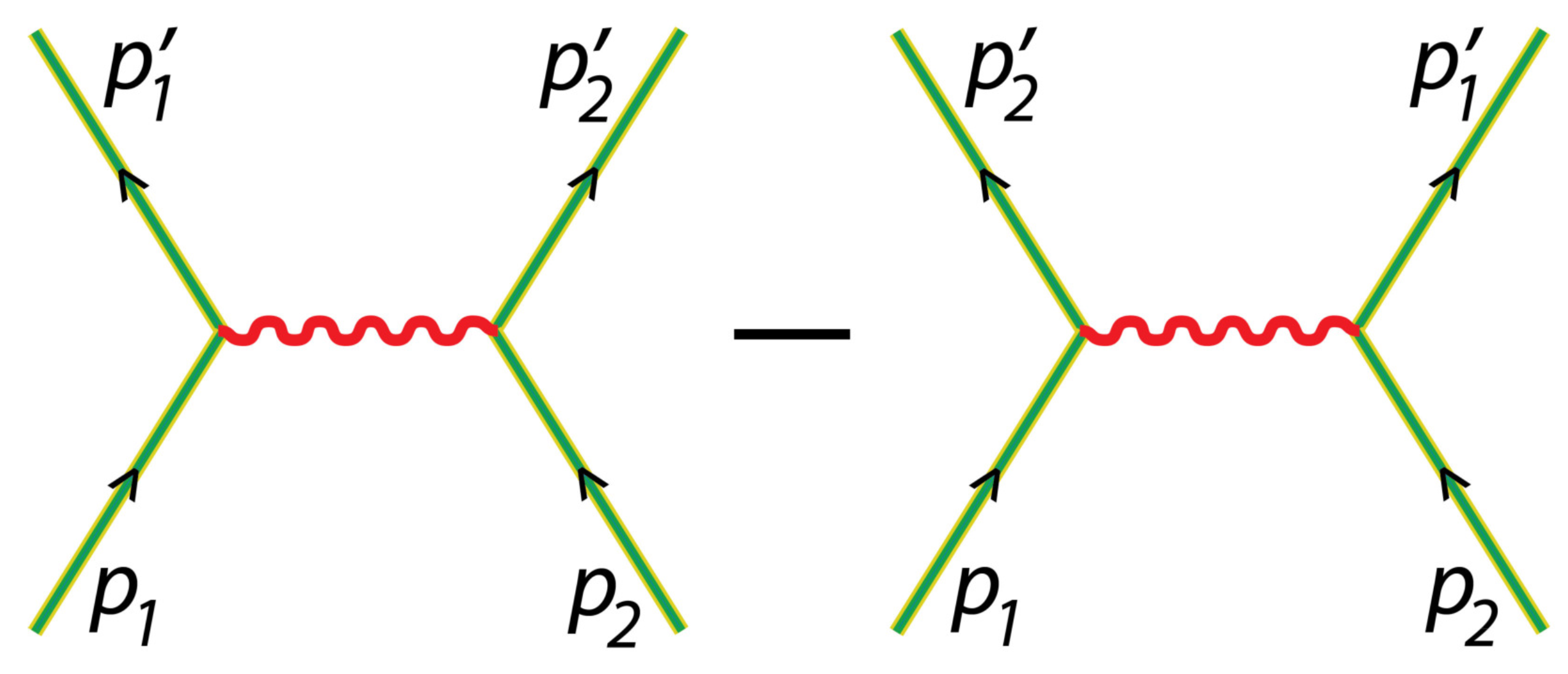
Let us start by considering two electrons with (field-free) four-momenta $p_1$ and $p_2$ in a relativistically intense train of laser pulses of arbitrary polarization. Similar to the case of Compton scattering (see Section 4), our approach considers that the electrons interact with a classical vector potential and can absorb or emit N quantized modes of the field (photons). Hence, in the Furry picture, the electron states before and after the scattering event takes place, are described by the Volkov solution in Equation (35) with asymptotic four-momenta $p_1$ and $p_2$ (incoming particles) or $p_1^{\prime }$ and $p_2^{\prime }$ (outgoing particles). In Figure 2, we present the Feynman diagrams corresponding to the direct (Figure 2, left) and exchange (Figure 2, right) contributions to the Møller scattering. While the straight lines represent Volkov states labeled by different field-free momenta, the wiggly line corresponds to the exchange of a virtual photon. Due to the indistinguishability of electrons, both the direct and exchange contributions need to be accounted for. To obtain an explicit form of the scattering matrix element, the plane-wave-front approximation needs to be introduced. In such case, we represent the four-vector potential defining the field in the form of Equation (23). However, the functions $f_1(k·x)$ and $f_2(k·x)$ are periodic and do not vanish outside the interval $k·x\in [0,2\pi ]$.

As done in [28,103], the scattering matrix element in the laser-assisted Møller process can be calculated from the well-know formulas for the laser-free case (see, e.g., [104,105]). To this end, the field-free states of the electron are replaced by the Volkov solution. Hence, the probability amplitude for the problem in consideration is

$$\begin{array}{cc}\hfill {\mathcal{A}}^{(++)}({\mathit{p}}_1^{\prime }{\lambda }_1^{\prime },{\mathit{p}}_2^{\prime }{\lambda }_2^{\prime };{\mathit{p}}_1{\lambda }_1,{\mathit{p}}_2{\lambda }_2)=\frac{1}{\sqrt{2}}[& {\mathcal{A}}_{\mathrm{Dis}}^{(++)}({\mathit{p}}_1^{\prime }{\lambda }_1^{\prime },{\mathit{p}}_2^{\prime }{\lambda }_2^{\prime };{\mathit{p}}_1{\lambda }_1,{\mathit{p}}_2{\lambda }_2)\hfill \\ \hfill -& {\mathcal{A}}_{\mathrm{Dis}}^{(++)}({\mathit{p}}_2^{\prime }{\lambda }_2^{\prime },{\mathit{p}}_1^{\prime }{\lambda }_1^{\prime };{\mathit{p}}_1{\lambda }_1,{\mathit{p}}_2{\lambda }_2)].\hfill \end{array}$$

(82)

While the first term in the right-hand side of this equation accounts for the direct process, the second term accounts for the exchange one. The partial (distinguishable) amplitudes ${\mathcal{A}}_{\mathrm{Dis}}^{(++)}$ correspond to each individual Feynman diagram in Figure 2 and are given by

$${\mathcal{A}}_{\mathrm{Dis}}^{(++)}\equiv {\mathcal{A}}_{\mathrm{Dis}}^{(++)}({\mathit{p}}_1^{\prime }{\lambda }_1^{\prime },{\mathit{p}}_2^{\prime }{\lambda }_2^{\prime };{\mathit{p}}_1{\lambda }_1,{\mathit{p}}_2{\lambda }_2)=-4\pi \mathrm{i}\alpha \int {\mathrm{d}}^{4}x{\mathrm{d}}^{4}y{\left[j_{{\mathit{p}}_1^{\prime }{\lambda }_1^{\prime },{\mathit{p}}_1{\lambda }_1}^{(++)}\right]}^{\mu }{\left[D_{\mathrm{F}}(x-y)\right]}_{\mu \nu }{\left[j_{{\mathit{p}}_2^{\prime }{\lambda }_2^{\prime },{\mathit{p}}_2{\lambda }_2}^{(++)}\right]}^{\nu }.$$

(83)

Here, $j_{{\mathit{p}}_1^{\prime }{\lambda }_1^{\prime },{\mathit{p}}_1{\lambda }_1}^{(++)}$ are the Volkov four-currents defined in Equation (39) and ${\lambda }_i$, ${\lambda }_i^{\prime }$, $i=1,2$ are the initial and final spin states of the electrons, respectively. Furthermore, ${\left[D_{\mathrm{F}}(x-y)\right]}_{\mu \nu }$ is the Feynman propagator, which we choose in the Feynman gauge,

$$\begin{array}{cc}\hfill {\left[D_{\mathrm{F}}(x-y)\right]}_{\mu \nu }=& \int \frac{{\mathrm{d}}^{4}K}{{\left(2\pi \right)}^4}\frac{g_{\mu \nu }}{K^2+\mathrm{i}0}{\mathrm{e}}^{-\mathrm{i}K·(x-y)}\equiv \int \frac{{\mathrm{d}}^{4}K}{{\left(2\pi \right)}^4}{\left[{\tilde{D}}_{\mathrm{F}}\left(K\right)\right]}_{\mu \nu }{\mathrm{e}}^{-\mathrm{i}K·(x-y)}.\hfill \end{array}$$

(84)

By inserting this expression into the distinguishable probability amplitude in Equation (83) and taking into account the explicit form of the Volkov four-currents in Equation (39), we obtain

$$\begin{array}{cc}\hfill {\mathcal{A}}_{\mathrm{Dis}}^{(++)}=\frac{-2\mathrm{i}\alpha }{{\left(2\pi \right)}^3}& \int {\mathrm{d}}^{4}x{\mathrm{d}}^{4}y{\mathrm{d}}^{4}K{\mathrm{e}}^{-\mathrm{i}K·(x-y)}\left[{\overline{\psi }}_{{\mathit{p}}_1^{\prime }{\lambda }_1^{\prime }}^{(+)}\left(x\right){\gamma }^{\mu }{\psi }_{{\mathit{p}}_1{\lambda }_1}^{(+)}\left(x\right)\right]{\left[{\tilde{D}}_{\mathrm{F}}\left(K\right)\right]}_{\mu \nu }\left[{\overline{\psi }}_{{\mathit{p}}_2^{\prime }{\lambda }_2^{\prime }}^{(+)}\left(y\right){\gamma }^{\nu }{\psi }_{{\mathit{p}}_2{\lambda }_2}^{(+)}\left(y\right)\right].\hfill \end{array}$$

(85)

As shown in the early works of Oleĭnik and Bös et al. (see Refs. [84,85,86,87]), the laser field modifies the effective mass and momenta of the two electrons. For this reason, we introduce the dressed four-momentum $\overline{p}$, and effective mass ${\overline{m}}_{\mathrm{e}}$, which we define as [70]

$$\overline{p}=p+{\left(m_{\mathrm{e}}c\mu \right)}^2\frac{\langle f_1^2\rangle +\langle f_2^2\rangle }{2k·p}k,\mathrm{and}{\overline{m}}_{\mathrm{e}}^2=m_{\mathrm{e}}^2[1+{\mu }^2(\langle f_1^2\rangle +\langle f_2^2\rangle )],$$

(86)

where ${\overline{p}}_i$ ($i=1,2$) satisfy the relation ${\overline{p}}_i·{\overline{p}}_i={\overline{m}}_{\mathrm{e}}^2{c}^2$ [39,86,87]. Note that $\overline{p}$ is a particular case of the more general laser-dressed four momentum, defined in Equation (59), when $\langle f_1\rangle$ and $\langle f_2\rangle$ vanish. This happens for the infinite train of pulses considered here. It is possible now to write the Volkov states in Equation (85) in terms of the initial and final dressed four momenta. In such case, the Volkov current operator reads (see Equations (37) and (38))

$$\begin{array}{cc}\hfill {\overline{\psi }}_{{\mathit{p}}^{\prime }{\lambda }^{\prime }}^{(+)}\left(x\right){\gamma }^{\mu }{\psi }_{\mathit{p}\lambda }^{(+)}\left(x\right)=& \frac{m_{\mathrm{e}}c}{V\sqrt{p^0{p}^{\prime 0}}}{\overline{u}}_{{\mathit{p}}^{\prime }{\lambda }^{\prime }}^{(+)}\left(1+\frac{e\cancel{A}\cancel{k}}{2p^{\prime }·k}\right){\gamma }^{\mu }\left(1-\frac{e\cancel{A}\cancel{k}}{2p·k}\right)u_{\mathit{p}\lambda }^{(+)}\hfill \\ \hfill \times & exp\left[\mathrm{i}({\overline{p}}^{\prime }-\overline{p})·x-\mathrm{i}{Q}_{p^{\prime },p}(k·x)\right].\hfill \end{array}$$

(87)

Here, we introduce the functions $Q_{p^{\prime },p}(k·x)$, which for the laser field in Equation (23) is given by

$$\begin{array}{cc}\hfill Q_{p^{\prime },p}(k·x)=& \mu m_{\mathrm{e}}c{\int }_0^{k·x}\mathrm{d}\varphi \{f_1\left(\varphi \right)\left(\frac{{\epsilon }_1·p^{\prime }}{k·p^{\prime }}-\frac{{\epsilon }_1·p}{k·p}\right)+f_2\left(\varphi \right)\left(\frac{{\epsilon }_2·p^{\prime }}{k·p^{\prime }}-\frac{{\epsilon }_2·p}{k·p}\right)\hfill \\ \hfill -& \frac{{\left(\mu m_{\mathrm{e}}c\right)}^2}{2}[f_1^2\left(\varphi \right)-\langle f_1^2\rangle +f_2^2\left(\varphi \right)-\langle f_2^2\rangle ]\left(\frac{1}{k·p^{\prime }}-\frac{1}{k·p}\right)\}.\hfill \end{array}$$

(88)

As shown in Refs. [28,70,103], due to the periodicity of the vector potential and the Volkov solution, it is possible to perform the Fourier expansion of the four-current in Equation (87). In doing so, we write

$${\left[f_1(k·x)\right]}^n{\left[f_2(k·x)\right]}^m{\mathrm{e}}^{-\mathrm{i}{Q}_{p^{\prime },p}(k·x)}=\sum _{N=-\infty }^{\infty }{Q}_N^{(n,m)}{\mathrm{e}}^{-\mathrm{i}Nk·x},$$

(89)

where n and m can be 0, 1 or 2. With this in mind, we find that the four-current is given by

$${\overline{\psi }}_{{\mathit{p}}^{\prime }{\lambda }^{\prime }}^{(+)}\left(x\right){\gamma }^{\mu }{\psi }_{\mathit{p}\lambda }^{(+)}\left(x\right)=\frac{m_{\mathrm{e}}c}{V\sqrt{p^0{p}^{\prime 0}}}\sum _N{\mathrm{e}}^{\mathrm{i}({\overline{p}}^{\prime }-\overline{p}-Nk)·x}{\mathsf{\Phi }}_N^{\mu }(p^{\prime },p),$$

(90)

where the Fourier coefficients ${\mathsf{\Phi }}_N^{\mu }(p^{\prime },p)$ are

$$\begin{array}{c}{\mathsf{\Phi }}_N^{\mu }(p^{\prime },p)={\overline{u}}_{{\mathit{p}}^{\prime }{\lambda }^{\prime }}^{(+)}\{{\gamma }^{\mu }{Q}_N^{(0,0)}-\frac{\mu m_{\mathrm{e}}c}{2}{Q}_N^{(1,0)}\left(\frac{{\cancel{\epsilon }}_1\cancel{k}}{k·p^{\prime }}{\gamma }^{\mu }-{\gamma }^{\mu }\frac{{\cancel{\epsilon }}_1\cancel{k}}{k·p}\right)-\frac{\mu m_{\mathrm{e}}c}{2}{Q}_N^{(0,1)}\left(\frac{{\cancel{\epsilon }}_2\cancel{k}}{k·p^{\prime }}{\gamma }^{\mu }-{\gamma }^{\mu }\frac{{\cancel{\epsilon }}_2\cancel{k}}{k·p}\right)\hfill \\ -\frac{{\left(\mu m_{\mathrm{e}}c\right)}^2}{4(k·p^{\prime })(k·p)}\left[Q_N^{(2,0)}{\cancel{\epsilon }}_1\cancel{k}{\gamma }^{\mu }{\cancel{\epsilon }}_1\cancel{k}+Q_N^{(1,1)}({\cancel{\epsilon }}_1\cancel{k}{\gamma }^{\mu }{\cancel{\epsilon }}_2\cancel{k}+{\cancel{\epsilon }}_2\cancel{k}{\gamma }^{\mu }{\cancel{\epsilon }}_1\cancel{k})+Q_N^{(0,2)}{\cancel{\epsilon }}_2\cancel{k}{\gamma }^{\mu }{\cancel{\epsilon }}_2\cancel{k}\right]\}{u}_{\mathit{p}\lambda }^{(+)}.\hfill \end{array}$$

(91)

With the help of Equations (90) and (91), it is possible to rewrite the distinguishable probability amplitude in Equation (85) in the following way,

$$\begin{array}{cc}\hfill {\mathcal{A}}_{\mathrm{Dis}}^{(++)}=& \frac{-2\mathrm{i}\alpha }{{\left(2\pi \right)}^3}\frac{m_{\mathrm{e}}^2{c}^2}{V^2\sqrt{p_1^0{p_1^{\prime }}^0{p}_2^0{p_2^{\prime }}^0}}\sum _{N_1}\sum _{N_2}\int {\mathrm{d}}^{4}x{\mathrm{d}}^{4}y{\mathrm{d}}^{4}K{\left[{\tilde{D}}_{\mathrm{F}}\left(K\right)\right]}_{\mu \nu }{\mathrm{e}}^{\mathrm{i}({\overline{p}}_1^{\prime }-{\overline{p}}_1-N_{1}k-K)·x}\hfill \\ \hfill \times & {\mathrm{e}}^{\mathrm{i}({\overline{p}}_2^{\prime }-{\overline{p}}_2-N_{2}k+K)·y}{\mathsf{\Phi }}_{N_1}^{\mu }(p_1^{\prime },p_1){\mathsf{\Phi }}_{N_2}^{\nu }(p_2^{\prime },p_2).\hfill \end{array}$$

(92)

The integration over ${\mathrm{d}}^{4}x$ leads to a four-dimensional delta function, which allows us to perform the integral over ${\mathrm{d}}^{4}K$ directly. Finally, we arrive at the following expression,

$$\begin{array}{cc}\hfill {\mathcal{A}}_{\mathrm{Dis}}^{(++)}=& \frac{-4\pi \mathrm{i}\alpha m_{\mathrm{e}}^2{c}^2{\left(2\pi \right)}^4}{V^2\sqrt{p_1^0{p_1^{\prime }}^0{p}_2^0{p_2^{\prime }}^0}}\sum _{N_1}\sum _{N_2}{\delta }^{\left(4\right)}({\overline{p}}_1+{\overline{p}}_2-{\overline{p}}_1^{\prime }-{\overline{p}}_2^{\prime }+(N_1+N_2)k){\left[{\tilde{D}}_{\mathrm{F}}({\overline{p}}_2-{\overline{p}}_2^{\prime }+N_{2}k)\right]}_{\mu \nu }\hfill \\ \hfill \times & {\mathsf{\Phi }}_{N_1}^{\mu }(p_1^{\prime },p_1){\mathsf{\Phi }}_{N_2}^{\nu }(p_2^{\prime },p_2).\hfill \end{array}$$

(93)

Hence, the Møller probability amplitude accounting for the indistinguishability of the electrons [Equation (82)] is given by

$$\begin{array}{cc}\hfill {\mathcal{A}}^{(++)}({\mathit{p}}_1^{\prime }{\lambda }_1^{\prime },{\mathit{p}}_2^{\prime }{\lambda }_2^{\prime };{\mathit{p}}_1{\lambda }_1,{\mathit{p}}_2{\lambda }_2)=& \frac{-4\pi \mathrm{i}\alpha m_{\mathrm{e}}^2{c}^2{\left(2\pi \right)}^4}{V^2\sqrt{2p_1^0{p_1^{\prime }}^0{p}_2^0{p_2^{\prime }}^0}}\sum _N{\delta }^{\left(4\right)}({\overline{p}}_1+{\overline{p}}_2-{\overline{p}}_1^{\prime }-{\overline{p}}_2^{\prime }+Nk)t_N(p_1^{\prime },p_2^{\prime },p_1,p_2),\hfill \end{array}$$

(94)

where the matrix elements $t_N(p_1^{\prime },p_2^{\prime },p_1,p_2)$ are

$$\begin{array}{cc}\hfill t_N(p_1^{\prime },p_2^{\prime },p_1,p_2)=& \sum _M[{\left[{\tilde{D}}_{\mathrm{F}}({\overline{p}}_2-{\overline{p}}_2^{\prime }+Mk)\right]}_{\mu \nu }{\mathsf{\Phi }}_{N-M}^{\mu }(p_1^{\prime },p_1){\mathsf{\Phi }}_M^{\nu }(p_2^{\prime },p_2)\hfill \\ \hfill -& {\left[{\tilde{D}}_{\mathrm{F}}({\overline{p}}_2-{\overline{p}}_1^{\prime }+Mk)\right]}_{\mu \nu }{\mathsf{\Phi }}_{N-M}^{\mu }(p_2^{\prime },p_1){\mathsf{\Phi }}_M^{\nu }(p_1^{\prime },p_2)].\hfill \end{array}$$

(95)

Note that, for each term in the sum in Equation (94), the four-dimensional delta function establishes the energy and momentum conservation relations

$${\overline{p}}_1+{\overline{p}}_2-{\overline{p}}_1^{\prime }-{\overline{p}}_2^{\prime }+Nk=0.$$

(96)

Once the probability amplitude for the Møller process is obtained [Equation (94)], it is possible to calculate the corresponding Nth order cross-section ${\sigma }_N^{\mathrm{M}ø\mathrm{ll}.}$ in the following way [28,103],

$$\begin{array}{cc}\hfill {\sigma }_N^{\mathrm{M}ø\mathrm{ll}.}=\frac{2{\left(m_{\mathrm{e}}c\right)}^4{\alpha }^2}{\sqrt{{(p_1·p_2)}^2-{\left(m_{\mathrm{e}}c\right)}^4}}& \int \frac{{\mathrm{d}}^3{p}_1^{\prime }}{{p_1^{\prime }}^0}\frac{{\mathrm{d}}^3{p}_2^{\prime }}{{p_2^{\prime }}^0}{\delta }^{\left(4\right)}({\overline{p}}_1+{\overline{p}}_2-{\overline{p}}_1^{\prime }-{\overline{p}}_2^{\prime }+Nk){\left|t_N(p_1^{\prime },p_2^{\prime },p_1,p_2)\right|}^2.\hfill \end{array}$$

(97)

The integration over ${\mathrm{d}}^3{p}_2^{\prime }$ can be performed by calculating the Jacobian $J({\overline{p}}_2^{\prime },p_2^{\prime })$ (for details see, e.g., Ref. [28]). Hence, the corresponding differential cross-section is given by

$$\begin{array}{cc}\hfill \frac{{\mathrm{d}}^2{\sigma }_N^{\mathrm{M}ø\mathrm{ll}.}}{\mathrm{d}{\mathsf{\Omega }}_{{\mathit{p}}_1^{\prime }}}=& {\int }_0^{\infty }\mathrm{d}|{\mathit{p}}_1^{\prime }\left|\right|{\mathit{p}}_1^{\prime }{|}^2\frac{2{\left(m_{\mathrm{e}}c\right)}^4{\alpha }^2}{\sqrt{{(p_1·p_2)}^2-{\left(m_{\mathrm{e}}c\right)}^4}}\frac{J({\overline{p}}_2^{\prime },p_2^{\prime })}{{p_1^{\prime }}^0{p_2^{\prime }}^0}\hfill \\ \hfill \times & {\delta }^{\left(1\right)}({\overline{p}}_1^0+{\overline{p}}_2^0-{\overline{p}}_1^{\prime 0}-{\overline{p}}_2^{\prime 0}+N{k}^0){\left|t_N(p_1^{\prime },p_2^{\prime },p_1,p_2)\right|}^2,\hfill \end{array}$$

(98)

where $\mathrm{d}{\mathsf{\Omega }}_{{\mathit{p}}_1^{\prime }}$ is the solid angle of electrons scattering with momentum ${\mathit{p}}_1^{\prime }$. Finally, after integrating over $p_1^{\prime }$, we arrive at the Nth photon differential cross-section

$$\begin{array}{c}\hfill \frac{{\mathrm{d}}^2{\sigma }_N^{\mathrm{M}ø\mathrm{ll}.}}{\mathrm{d}{\mathsf{\Omega }}_{{\mathit{p}}_1^{\prime }}}=\frac{2{\left(m_{\mathrm{e}}c\right)}^4{\alpha }^2}{\sqrt{{(p_1·p_2)}^2-{\left(m_{\mathrm{e}}c\right)}^4}}\frac{J({\overline{p}}_2^{\prime },p_2^{\prime })}{{p_2^{\prime }}^0}|{\mathit{p}}_1^{\prime }\left|\right|\frac{\mathrm{d}{p_1^{\prime }}^0}{\mathrm{d}{\overline{p}}_1^{\prime 0}}|{\left|t_N(p_1^{\prime },p_2^{\prime },p_1,p_2)\right|}^2.\end{array}$$

(99)

The resonance phenomena is observed when $|t_N(p_1^{\prime },p_2^{\prime },p_1,p_2){|}^2$ becomes singular. From its definition [Equation (95)], we can see that this happens at the incoming and outgoing momenta when ${\left[{\tilde{D}}_{\mathrm{F}}\right]}_{\mu \nu }$ also becomes singular [see Equation (84)]. This means that the relations

$${({\overline{p}}_2-{\overline{p}}_2^{\prime }+M_{2}k)}^2=0\mathrm{or}{({\overline{p}}_2-{\overline{p}}_1^{\prime }+M_{2}k)}^2=0$$

(100)

determine the resonances for a given integer value $M_2$. For simplicity, let us consider only the first of those equations. We define the four vector $k^{\prime }$ as

$$k^{\prime }={\overline{p}}_2-{\overline{p}}_2^{\prime }+M_{2}k,$$

(101)

and, therefore, we are interested in the condition $k^{\prime 2}=0$. From the energy-momentum conservation relations in Equation (96), one can write $k^{\prime }$ in terms of ${\overline{p}}_1$ and ${\overline{p}}_1^{\prime }$, namely

$$k^{\prime }={\overline{p}}_1^{\prime }-{\overline{p}}_1-M_{1}k,$$

(102)

where $M_1+M_2=N$.

Due to the symmetry of the problem, it is possible to introduce a particular frame of reference to analyze the resonance phenomena [28,103]. In particular, we consider the center-of-mass frame, where both electrons have opposite momenta and travel along the z-direction. On the other hand, the laser field is assumed to propagate in the $xz$-plane at an angle $\theta$ with respect to the z-axis. This means that $p_1$, $p_2$ and k are given by

$$\begin{array}{c}\hfill p_1=(p^0,0,0,p),p_2=(p^0,0,0,-p),\mathrm{and}k=\frac{\omega }{c}(1,sin\theta ,0,cos\theta ),\end{array}$$

(103)

where $\omega$ is the fundamental frequency of field oscillations (i.e., $k^0=\omega /c$) and $p=\sqrt{{\left(p^0\right)}^2-{\left(m_{\mathrm{e}}c\right)}^2}$. The four-vector $k^{\prime }$ can be written in terms of two parameters, $\zeta$ and $\xi$, as

$$k^{\prime }=\frac{{\omega }^{\prime }}{c}\left(1,\xi ,\pm \sqrt{1-{\xi }^2-{\zeta }^2},\zeta \right),$$

(104)

and, to guarantee that it is real, the condition ${\xi }^2+{\zeta }^2⩽1$ must be imposed. For our further derivations we also introduce two additional quantities, $p_{\pm }=p^0\pm pcos\theta$ and, from Equations (103) and (104), we write the following scalar products as

$$\begin{array}{cc}\hfill p_1·k=\frac{\omega }{c}{p}_{-},p_2·k=& \frac{\omega }{c}{p}_{+},p_1·k^{\prime }=\frac{{\omega }^{\prime }}{c}(p^0-p\zeta ),p_2·k^{\prime }=\frac{{\omega }^{\prime }}{c}(p^0+p\zeta ),\hfill \end{array}$$

(105)

$$\begin{array}{c}k·k^{\prime }=\frac{\omega {\omega }^{\prime }}{c^2}(1-\xi sin\theta -\zeta cos\theta ).\hfill \end{array}$$

(106)

From now on, we express the dressed four-momenta in terms of the ponderomotive energy of the electron in the laser field with $\langle f_1\rangle =\langle f_2\rangle =0$ [see Equation (63)],

$$U_p=\frac{e^2{A}_0^2}{2m_{\mathrm{e}}}(\langle f_1^2\rangle +\langle f_2^2\rangle ).$$

(107)

With this in mind, we write

$$\begin{array}{c}\hfill {\overline{p}}_i=p_i+\frac{m_{\mathrm{e}}{U}_p}{k·p_i}k\mathrm{and}{\overline{p}}_i^{\prime }=p_i^{\prime }+\frac{m_{\mathrm{e}}{U}_p}{k·p_i^{\prime }}k,\end{array}$$

(108)

for $i=1,2$. The final (asymptotic) momenta $p_1^{\prime }$ and $p_2^{\prime }$ are on the mass shell, so the relations

$$p_1^{\prime }·p_1^{\prime }=m_{\mathrm{e}}^2{c}^2\mathrm{and}{p}_2^{\prime }·p_2^{\prime }=m_{\mathrm{e}}^2{c}^2$$

(109)

are also satisfied. By making use of Equations (101), (102), and (108), Equation (109) lead to

$$M_1{p}_1·k+\left[p_1+\frac{m_{\mathrm{e}}{U}_p}{2p_1·k}k\right]·k^{\prime }+M_{1}k·k^{\prime }=0$$

(110)

and

$$-M_2{p}_2·k+\left[p_2+\frac{m_{\mathrm{e}}{U}_p}{2p_2·k}k\right]·k^{\prime }+M_{2}k·k^{\prime }=0.$$

(111)

With the help of Equations (105) and (106), it is possible to rewrite Equations (110) and (111) in terms of $\xi$, $\zeta$ and $p_{\pm }$. As done in Refs. [28,103], the two resulting equations can be combined to give the following expression,

$$A\xi +B\zeta +C=0,$$

(112)

with

$$A=-\left[m_{\mathrm{e}}{U}_p\left(M_2\frac{p_{+}}{p_{-}}+M_1\frac{p_{-}}{p_{+}}\right)+2M_1{M}_2\frac{p^0\omega }{c}\right]sin\theta ,$$

(113)

$$B=(M_1{p}_{-}-M_2{p}_{+})p-\left[m_{\mathrm{e}}{U}_p\left(M_2\frac{p_{+}}{p_{-}}+M_1\frac{p_{-}}{p_{+}}\right)+2M_1{M}_2\frac{p^0\omega }{c}\right]cos\theta ,$$

(114)

and

$$C=(M_2{p}_{+}+M_1{p}_{-})p^0+m_{\mathrm{e}}{U}_p\left(M_2\frac{p_{+}}{p_{-}}+M_1\frac{p_{-}}{p_{+}}\right)+2M_1{M}_2\frac{p^0\omega }{c}.$$

(115)

Note that the linear Equation (112) determines the conditions imposed on $\xi$ and $\zeta$ to observe resonances. Furthermore, it is known that the distance D from the origin of the $\xi \zeta$-plane to the line defined by Equation (112) is given by

$$D=\frac{\left|C\right|}{\sqrt{A^2+B^2}}.$$

(116)

As discussed above, the inequality ${\xi }^2+{\zeta }^2⩽1$ also needs to be fulfilled. This defines a disk of radius 1 in the same plane, thus the additional condition $D⩽1$ needs to be imposed. In other words, given the initial parameters of the laser field and electron momenta, the function

$$f(M_1,M_2)=C^2-(A^2+B^2),$$

(117)

determines the sets of values $(M_1,M_2)$ for which resonances can take place, i.e., the pair of integers for which $f(M_1,M_2)⩽0$. Once the possible $M_1$ and $M_2$ are found, the total number of photons absorbed or emitted during the Møller scattering is known ($N=M_1+M_2$) and the frequency ${\omega }^{\prime }$ can be calculated. As discussed in Refs. [28,103], the values of $\xi$ and $\zeta$ at fixed $M_1$ and $M_2$ are found by introducing the parameter $0⩽\beta ⩽2\pi$. Namely,

$$\xi \left(\beta \right)=-\frac{1}{A^2+B^2}\left(B\sqrt{A^2+B^2-C^2}cos\beta -AC\right)$$

(118)

and

$$\zeta \left(\beta \right)=\frac{1}{A^2+B^2}\left(A\sqrt{A^2+B^2-C^2}cos\beta +BC\right).$$

(119)

Hence, from Equation (104), the four-vector $k^{\prime }\left(\beta \right)$ is determined. By making use of Equations (101) and (102), and for the given initial conditions, the final dressed momenta ${\overline{p}}_1^{\prime }$ and ${\overline{p}}_2^{\prime }$ are calculated which, at the same time, determines $p_1^{\prime }$ and $p_2^{\prime }$.

In conclusion, by following the derivations in Refs. [28,103], we have found the Nth-order differential cross-section in the non-linear laser-assisted Møller scattering. The laser field was modeled as an infinite and periodic series of pulses of arbitrary polarization. Similar to the early works of Oleĭnik and Bös et al. [84,85,86,87] or Bergou et al. [88], we determine the conservation relations satisfied by the dressed momenta and the dynamical parameters which play a role in the resonant scattering process. The conditions necessary for the observation of resonances are established.

6. Mott Scattering

Already in 1964, S. Rand analyzed the photon absorption during the scattering of an electron by a positively charged particle in the presence of an electromagnetic field (also known as the inverse bremsstrahlung mechanism) [106]. In this reference, he calculated the frequency dependence of the absorption cross-section from a non-relativistic point of view by using an oscillating frame of reference. A year later, Bunkin and Fedorov [107] reconsidered the problem from a more convenient perspective; while paying close attention to the multiphoton emission or absorption, they calculated the transition probability and scattering cross-section associated with the exchange of a well-defined number of photons with the electromagnetic radiation. Their treatment, also in the non-relativistic regime, was based on the dipole approximation of the monochromatic plane laser wave. The initial and final electron states were represented by the Volkov solution of the Schrödinger equation in the electromagnetic field (see also [108] and references therein). In 1973, Kroll and Watson studied the radiation-assisted electron scattering for the emission (absorption) of multiple photons [109]. The authors also calculated the non-relativistic multiquantum differential cross-section restricted to the case of weak scattering potentials or large wavelengths of the field. Lami and Rahman [108] analyzed the electron scattering by a hydrogen atom in a laser field of low intensity. As they showed, this process could be used to examine the atomic structure of the target (see also the previous works by Rahman and Faisal [110] and Gavrila and van der Wiel [111] together with the references therein). In 1984 Gavrila and Kamiński [112] developed further an approach, previously introduced by Gersten and Mittleman [113], to study the electron scattering by an atom (free-free transitions) in high-intensity and short wavelength laser fields. Using the Krammers-Henneberger frame, they demonstrated that under such circumstances the nth-order differential cross-section can be calculated from a convergent series with a dominant term. Furthermore, it was shown there that the electron experiences an effective (dressed) potential rather than the pure atomic one. Dimou and Faisal [114] reconsidered the electron scattering by $H^{+}$ ions and predicted the appearance of a different type of resonances occurring at low electron kinetic energies. Those resonances were attributed to momentary transitions to bound (Rydberg) states prior to the electron promotion to the continuum. (For a detailed analysis of free-free transitions in the laser field, we also refer the reader to the book by Faisal [115].)

The laser radiation available in the early 1980s was characterized by a finite frequency bandwidth and “chaotic fluctuations” of phase and amplitude [116]. For this reason, it was important to take into account the statistical properties of the light in scattering processes. To this end, in 1980, Zoller [117] examined the contribution of multimode laser fields over the non-linear differential cross-section. Daniele et al. [118] centered their attention on the influence of the frequency bandwidth in a chaotic electromagnetic field over the free-free transitions. Trombetta et al. [119] considered the “phase diffusion model” by assuming that the radiation phase undergoes random changes while its amplitude is approximately stable. Francken and Joachain [120] based their analysis on the so-called “random telegraph” model, which considers variations of the phase, amplitude and frequency of the radiation as Markovian processes with random fluctuations between two allowed states. Finally, in 1988 Kamiński [116] generalized the Kroll-Watson formula to account for any arbitrary stochastic model describing the low-frequency laser field.

With respect to the relativistic quantum treatment of laser-assisted Mott scattering, we mention the early work of Denisov and Fedorov [121]. The authors used the relativistic form of the Volkov solution and considered the field as a classical monochromatic plane wave of elliptical polarization to calculate the non-linear cross-sections. Almost 20 years later, Kamiński [122] reconsidered the scattering of a charged particle by a central potential in a linearly-polarized laser field. The extension of the Kroll-Watson formula to the relativistic case was also derived there. Already at the beginning of the 1990s, Gorodnitskiĭ et al. [123] and Roshchupkin [124,125] published a series of papers regarding the free-free transitions under the combined action of two light fields. For a particular configuration, the authors analyzed the interference effects arising from the contribution of the two fields. In Ref. [125], special emphasis was put on the influence of the electron velocity regime on the scattering angle, meaning that, while ultra-relativistic particles are mostly detected in the direction of propagation of the radiation, the non-relativistic ones are observed at angles that depend on the initial geometry of the collision. A review article concerning free-free transitions in the presence of bichromatic fields was presented by Ehlotzky [126]. Szymanowski et al. [127] considered the scattering problem in very intense circularly-polarized laser fields. They compared the results from the relativistic treatments based on the Dirac and Klein-Gordon equations, and the non-relativistic ones based on the Schrödinger equation. Such comparison allowed the authors to determine the influence of radiation pressure, relativistic mass, and spin–orbit and spin–light coupling on the scattering dynamics. It is known that in many processes involving the interactions of electrons and ions (photoionization, for instance) the Coulomb potential can play an important role during the evolution of the system. For this reason, Li et al. [128] analyzed the Coulomb effect over the free-free transitions in a linearly-polarized monochromatic plane wave of moderate intensity. The authors showed that the electron-ion interaction may increase the resulting cross-section at certain range of scattering angles (see also Ref. [129]). Additionally, in Ref. [130], Ngoko Djiokap et al. considered, besides the contribution from the Coulomb field, the influence of the “anomalous magnetic moment” of the electron. Recently, due to the necessity to develop a new theoretical framework to account for the short duration of single laser pulses, Boca [129] examined the scattering of a Klein-Gordon particle in such type of fields. In this reference, the effect of the pulse duration, intensity and envelope shape over the differential cross-section was determined. The same author also studied the case of free-free transitions of a fermion in the light pulse [131]. In recent years, Lebed’ [132,133] and Lebed’ and Roshchupkin [134] centered their attention on the Mott scattering assisted by pulses of electromagnetic radiation (see also the reviews [101,102]). In particular, the use of circularly-polarized bichromatic laser fields and the interference effects associated to them are described in Refs. [132,134]. In Ref. [133], the light field is modeled as a single non-monochromatic wave. The authors considered long-in-time pulses such that the “quasi-monochromatic approximation” becomes valid.

In the period 1998–2009, a series of papers by Panek et al. [135,136] and Kamiński et al. [137], and review articles by Ehlotzky et al. [28,138] were published. There, the electron–atom scattering in linearly-polarized and intense laser fields was considered. The electromagnetic radiation was approximated as a monochromatic plane wave. It is the aim of this section to present the analytical derivations introduced in [28,135,137] for a more general non-monochromatic and periodic laser field of infinite duration and arbitrary polarization. Details of the derivations can be found in the aforementioned references.

We consider here the interaction of an electron (four-momentum p and spin state $\lambda$) with an isolated atom in the presence of a relativistically-intense plane wave. While the atom is described by a screened Coulomb potential with a screen length ℓ, i.e.,

$$e{A}_{\mathrm{SC}}^{\mu }\left(x\right)=-Z\alpha c\frac{{\mathrm{e}}^{-\left|\mathit{x}\right|/\ell }}{\left|\mathit{x}\right|}{g}^{\mu 0}\equiv \frac{1}{c}V\left(\mathit{x}\right)g^{\mu 0}$$

(120)

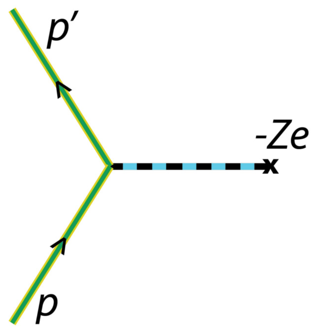
the laser field is defined by the four-vector potential in Equation (23). Note that, in the present calculations, the functions $f_1(k·x)$ and $f_2(k·x)$ are assumed to be periodic and do not vanish for $k·x<0$ and $k·x>2\pi$. The final electron four-momentum will be denoted as $p^{\prime }$ and its spin state as ${\lambda }^{\prime }$. As done for the laser-assisted Compton and Møller processes, the Mott scattering is treated in the Furry picture and plane-wave-fronted pulse approximation. In other words, the initial and final electron states are the Volkov solution in Equation (35) labeled by the field-free momenta $\mathit{p}$ and ${\mathit{p}}^{\prime }$, respectively. This corresponds to the Feynman diagram shown in Figure 3. Under those circumstances, and in the first Born approximation, the probability amplitude of Mott scattering, ${\mathcal{A}}_{\mathrm{M}}^{(++)}({\mathit{p}}^{\prime }{\lambda }^{\prime },\mathit{p}\lambda )$, is given by

$$\begin{array}{cc}\hfill {\mathcal{A}}_{\mathrm{M}}^{(++)}({\mathit{p}}^{\prime }{\lambda }^{\prime },\mathit{p}\lambda )=& -\mathrm{i}\int {\mathrm{d}}^{4}x{\left[j_{{\mathit{p}}^{\prime }{\lambda }^{\prime },\mathit{p}\lambda }^{(++)}\left(x\right)\right]}_{\mu }e{A}_{\mathrm{SC}}^{\mu }\left(x\right)=-\frac{\mathrm{i}}{c}\int {\mathrm{d}}^{4}x{\left[j_{{\mathit{p}}^{\prime }{\lambda }^{\prime },\mathit{p}\lambda }^{(++)}\left(x\right)\right]}_{0}V\left(\mathit{x}\right),\hfill \end{array}$$

(121)

where $j_{{\mathit{p}}^{\prime }{\lambda }^{\prime },\mathit{p}\lambda }^{(++)}\left(x\right)$ is the Volkov four-current in Equation (39). Hence, by inserting the analytical expression of the Volkov solution, we obtain

$$\begin{array}{cc}\hfill {\mathcal{A}}_{\mathrm{M}}^{(++)}({\mathit{p}}^{\prime }{\lambda }^{\prime },\mathit{p}\lambda )=& -\mathrm{i}\frac{m_{\mathrm{e}}}{V\sqrt{p^0{p}^{\prime 0}}}\int {\mathrm{d}}^{4}xexp\left(\mathrm{i}[S_{p^{\prime }}^{(+)}\left(x\right)-S_p^{(+)}\left(x\right)]\right)\hfill \\ \hfill \times & \left[{\overline{u}}_{{\mathit{p}}^{\prime }{\lambda }^{\prime }}^{(+)}\left(1+\frac{e\cancel{A}\cancel{k}}{2p^{\prime }·k}\right){\gamma }^{0}V\left(\mathit{x}\right)\left(1-\frac{e\cancel{A}\cancel{k}}{2p·k}\right)u_{\mathit{p}\lambda }^{(+)}\right].\hfill \end{array}$$

(122)

In the following, we proceed in a similar way as for the Møller scattering (see Section 5). Namely, we introduce the dressed four-momenta $\overline{p}$ and ${\overline{p}}^{\prime }$ as defined in Equation (86) and the function $Q_{p^{\prime },p}(k·x)$ [Equation (88)] with the Fourier decomposition in Equation (89). Hence, the probability amplitude for Mott scattering is given by the infinite sum

$$\begin{array}{cc}\hfill {\mathcal{A}}_{\mathrm{M}}^{(++)}({\mathit{p}}^{\prime }{\lambda }^{\prime },\mathit{p}\lambda )& =-\mathrm{i}\frac{m_{\mathrm{e}}}{V\sqrt{p^0{p}^{\prime 0}}}\sum _{N=-\infty }^{\infty }\int {\mathrm{d}}^{4}x{\mathrm{e}}^{\mathrm{i}({\overline{p}}^{\prime }-\overline{p}-Nk)·x}{\mathsf{\Phi }}_N^0(p^{\prime },p)V\left(\mathit{x}\right),\hfill \end{array}$$

(123)

where ${\mathsf{\Phi }}_N^0(p^{\prime },p)$ is the zeroth-component of the coefficients given in Equation (91). Note that, while the integration is performed over the four space-time coordinates, the static potential depends only on the three spatial ones. For this reason, we write

$$\begin{array}{cc}\hfill {\mathcal{A}}_{\mathrm{M}}^{(++)}({\mathit{p}}^{\prime }{\lambda }^{\prime };\mathit{p}\lambda )=& -\mathrm{i}\frac{m_{\mathrm{e}}}{V\sqrt{p^0{p}^{\prime 0}}}\sum _N\int \mathrm{d}{x}^0{\mathrm{e}}^{\mathrm{i}[{\overline{p}}^{\prime 0}-{\overline{p}}^0-N{k}^0]x^0}\int {\mathrm{d}}^{3}xV\left(\mathit{x}\right){\mathrm{e}}^{-\mathrm{i}[{\overline{\mathit{p}}}^{\prime }-\overline{\mathit{p}}-N\mathit{k}]·\mathit{x}}{\mathsf{\Phi }}_N^0(p^{\prime },p)\hfill \\ \hfill =& -\mathrm{i}\frac{2\pi m_{\mathrm{e}}}{V\sqrt{p^0{p}^{\prime 0}}}\sum _N{\delta }^{\left(1\right)}[{\overline{p}}^{\prime 0}-{\overline{p}}^0-N{k}^0]\tilde{V}({\overline{\mathit{p}}}^{\prime }-\overline{\mathit{p}}-N\mathit{k}){\mathsf{\Phi }}_N^0(p^{\prime },p),\hfill \end{array}$$

(124)

where $\tilde{V}\left(\mathit{p}\right)$ is the Fourier transform of the potential energy. Next, as it is assumed that the electromagnetic radiation is periodic and lasts for a very long time T, we proceed to calculate the transition rates $w_{\mathrm{M}}$

$$w_{\mathrm{M}}=\underset{T\to \infty }{lim}\frac{|{\mathcal{A}}_{\mathrm{M}}^{(++)}({\mathit{p}}^{\prime }{\lambda }^{\prime };\mathit{p}\lambda ){|}^2}{T}.$$

(125)

With this in mind, and taking into account that ${\delta }^{\left(1\right)}[{\overline{p}}^{\prime 0}-{\overline{p}}^0-N_1{k}^0]\times {\delta }^{\left(1\right)}[{\overline{p}}^{\prime 0}-{\overline{p}}^0-N_2{k}^0]=0$ for $N_1\ne N_2$, we find that the transition rates for the laser-assisted Mott scattering in the field in Equation (23) are given by

$$w_{\mathrm{M}}=\frac{2\pi m_{\mathrm{e}}^{2}c}{V^2{p}^0{p}^{\prime 0}}\sum _N{\delta }^{\left(1\right)}[{\overline{p}}^{\prime 0}-{\overline{p}}^0-N{k}^0]|\tilde{V}({\overline{\mathit{p}}}^{\prime }-\overline{\mathit{p}}-N\mathit{k}){\mathsf{\Phi }}_N^0(p^{\prime },p){|}^2.$$

(126)

Up to now, we have presented a theoretical description of Mott scattering in non-monochromatic trains of laser pulses. It is worth mentioning that the laser-assisted Mott-like processes continue to attract a lot of attention. This is due to the analysis of fundamental phenomena happening, for instance, in plasma physics and cosmology. To this end, Hrour et al. [139] recently published a paper concerning the role played by the Coulomb interaction in proton–nucleus collisions in intense electromagnetic radiation. Du et al. [140] centered their attention in electron-muon scattering while focusing on the resonance phenomena. Bai et al. [141] have also considered the collision between muon neutrinos and electrons in the presence of electromagnetic radiation. The electron–proton scattering, where the target is not considered to be static, was treated by Liu et al. [142]. This is only to mention few works in this field that have been published recently.

In this section, we consider the electron scattering by a screened Coulomb potential in the presence of a light field. For sufficiently large initial kinetic energies, the results presented here are equally valid for the pure and screened Coulomb potentials. Note, however, that the theoretical treatment accounting for the electron interaction with the laser field and the pure Coulomb potential is still a challenging task and remains an open problem in the theoretical investigations of strong laser field-matter interactions.

7. Conclusions

In this review, we describe the behavior of a classical and quantum particle in the presence of electromagnetic radiation. Those results are used to analyze the non-linear Thomson and Compton scattering driven by single and arbitrarily short laser pulses. Other scattering phenomena, including Møller and Mott processes, are treated by considering non-monochromatic fields of infinite duration. As it mentioned above, due to the development of the new state-of-the-art laser facilities (which are capable of generating ultraintense and ultrashort pulses), it has become necessary to extend the previously known laser-assisted scattering theories to the case of short and highly non-monochromatic fields. To this end, Boca and Florescu [73] generalized the non-linear Compton scattering, and Boca [129,131] paved the road for a full generalization of the Mott scattering. However, further developments for the extension of Mott and Møller mechanisms are still necessary.

References

- Newton, R.G. Scattering Theory of Waves and Particles; Springer Science + Business Media: New York, NY, USA, 1982. [Google Scholar]
- Sharma, S.K.; Somerford, D.J. Light Scattering by Optically Soft Particles: Theory and Applications; Springer: Berlin/Heidelberg, Germany, 2006. [Google Scholar]
- Joachain, C.J.; Kylstra, N.J.; Potvliege, R.M. Atoms in Intense Laser Fields; Cambridge University Press: Cambridge, UK, 2012. [Google Scholar]
- Friedrich, H. Scattering Theory; Springer: Berlin/Heidelberg, Germany, 2016. [Google Scholar]
- Povh, B.; Rosina, M. Scattering and Structures: Essentials and Analogies in Quantum Physics; Springer: Berlin/Heidelberg, Germany, 2017. [Google Scholar]
- Hillas, A.M. Cosmic Rays, 1st ed.; Pergamon Press: Oxford, UK, 1972. [Google Scholar]
- Bonolis, L. Walther Bothe and Bruno Rossi: The birth and development of coincidence methods in cosmic-ray physics. Am. J. Phys. 2011, 79, 1133–1150. [Google Scholar] [CrossRef]
- NobelPrize.org. Nobel Media AB 2019. Victor F. Hess-Biographical. Available online: https://www.nobelprize.org/prizes/physics/1936/hess/biographical/ (accessed on 14 January 2019).
- NobelPrize.org. Nobel Media AB 2019. The Nobel Prize in Physics 1936. Available online: https://www.nobelprize.org/prizes/physics/1936/summary/ (accessed on 12 January 2019).
- Compton, A.H. The composition of cosmic rays. Proc. Am. Phil. Soc. 1935, 75, 251–274. [Google Scholar] [CrossRef]
- Bothe, W.; Kolhörster, W. Das Wesen der Höhenstrahlung. Z. Phys. 1929, 56, 751–777. [Google Scholar] [CrossRef]
- Kragh, H. Relativistic collisions: The work of Christian Møller in the early 1930s. Arch. Hist. Exact Sci. 1992, 43, 299–328. [Google Scholar] [CrossRef]
- Roqué, X. Møller scattering: A neglected application of early quantum electrodynamics. Arch. Hist. Exact Sci. 1992, 44, 197–264. [Google Scholar] [CrossRef]
- Mott, N.F. The scattering of fast electrons by atomic nuclei. Proc. R. Soc. Lond. A 1929, 124, 425–442. [Google Scholar] [CrossRef]
- Møller, C. Über den stoß zweier teilchen unter berücksichtigung der retardation der kräfte. Z. Phys. 1931, 70, 786–795. [Google Scholar] [CrossRef]
- Møller, C. Zur theorie des durchgangs schneller elektronen durch materie. Ann. Phys. 1932, 14, 531–585. [Google Scholar]
- Thomson, J.J. Conduction of Electricity Through Gases, 2nd ed.; Cambridge University Press: Cambridge, UK, 1906. [Google Scholar]
- Stuewer, R.H.; Cooper, M.J. History. In Compton Scattering; Williams, B., Ed.; McGraw-Hill: London, UK, 1977; pp. 1–27. [Google Scholar]
- Compton, A.H. A quantum theory of the scattering of X-rays by light elements. Phys. Rev. 1923, 21, 483–502. [Google Scholar] [CrossRef]
- Strickland, D.; Mourou, G. Compression of amplified chirped optical pulses. Opt. Commun. 1985, 56, 219–221. [Google Scholar] [CrossRef]
- NobelPrize.org. Nobel Media AB 2019. Press Release: The Nobel Prize in Physics 2018. Available online: https://www.nobelprize.org/prizes/physics/2018/press-release/ (accessed on 15 January 2019).
- Wolkow, D.M. Über eine klasse von lösungen der Diracschen Gleichung. Z. Phys. 1935, 94, 250. [Google Scholar] [CrossRef]
- Heinzl, T.; Seipt, D.; Kämpfer, B. Beam shape effects in nonlinear Compton and Thomson scattering. Phys. Rev. A 2010, 81, 022125. [Google Scholar] [CrossRef]
- Seipt, D.; Kämpfer, B. Nonlinear Compton scattering of ultrashort intense laser pulses. Phys. Rev. A 2011, 83, 022101. [Google Scholar] [CrossRef]
- Seipt, D.; Kämpfer, B. Scaling law for the photon spectral density in the nonlinear Thomson-Compton scattering. Phys. Rev. Spec. Top.-Accel. Beams 2011, 14, 040704. [Google Scholar] [CrossRef]
- Krajewska, K.; Kamiński, J.Z. Frequency scaling law for nonlinear Compton and Thomson scattering: Relevance of spin and polarization effects. Phys. Rev. A 2014, 90, 052117. [Google Scholar] [CrossRef]
- Krajewska, K.; Cajiao Vélez, F.; Kamiński, J.Z. Generalized Klein-Nishina formula. Phys. Rev. A 2015, 91, 062106. [Google Scholar] [CrossRef]
- Ehlotzky, F.; Krajewska, K.; Kamiński, J.Z. Fundamental processes of quantum electrodynamics in laser fields of relativistic power. Rep. Prog. Phys. 2009, 72, 046401. [Google Scholar] [CrossRef]
- Landau, L.D.; Lifshitz, E.M. The Classical Theory of Fields; Pergamon: New York, NY, USA, 1975. [Google Scholar]
- Ortner, J.; Rylyuk, V.M. Relativistic semiclassical approach in strong-field nonlinear photoionization. Phys. Rev. A 2000, 61, 033403. [Google Scholar] [CrossRef]
- Wooten, R.E.; Macek, J.H. Solutions of relativistic Newton’s equations for nonconstant fields. Am. J. Phys. 2004, 72, 998–1001. [Google Scholar] [CrossRef]
- Cajiao Vélez, F.; Kamiński, J.Z.; Krajewska, K. The spiral of life. J. Phys. Conf. Ser. 2018, 999, 012007. [Google Scholar] [CrossRef]
- Berestetski, V.; Lifchitz, E.; Pitayevski, L. Théorie Quantique Relativiste; MIR: Moscou, Russia, 1972. [Google Scholar]
- Bergou, J.; Varró, S. Wavefunctions of a free electron in an external field and their application in intense field interactions: II. Relativistic treatment. J. Phys. A Math. Gen. 1980, 13, 2823–2837. [Google Scholar] [CrossRef]
- Pardy, M. Massive photons and the Volkov solution. Int. J. Theor. Phys. 2004, 43, 127–139. [Google Scholar] [CrossRef]
- Varró, S. New exact solutions of the Dirac equation of a charged particle interacting with an electromagnetic plane wave in a medium. Laser Phys. Lett. 2013, 10, 095301. [Google Scholar] [CrossRef] [Green Version]
- Woodward, P.M. A method of calculating the field over a plane aperture required to produce a given polar diagram. J. Inst. Electr. Eng. Part IIIA 1946, 93, 1554–1558. [Google Scholar] [CrossRef]
- Lawson, J.D. Lasers and accelerators. IEEE Trans. Nuclear Sci. 1979, 26, 4217–4219. [Google Scholar] [CrossRef]
- Brown, L.S.; Kibble, T.W.B. Interaction of intense laser beams with electrons. Phys. Rev. A 1964, 133, 705–719. [Google Scholar] [CrossRef]
- Thomson, J.J. The Corpuscular Theory of Matter; Archibald Constable & Co., Ltd.: London, UK, 1907. [Google Scholar]
- McCormmach, R.J.J. Thomson and the structure of light. Br. J. Hist. Sci. 1967, 3, 362–387. [Google Scholar] [CrossRef]
- Sen Gupta, N.D. On the scattering of electromagnetic waves by free electron. Classical theory. Bull. Math. Soc. Calcutta 1949, 41, 187–198. [Google Scholar]
- Sen Gupta, N.D. On the scattering of electromagnetic waves by a free electron. Bull. Math. Soc. Calcutta 1952, 44, 175–180. [Google Scholar]
- Sen Gupta, N.D. Thomson scattering of high intensity beam with radiation reaction. Z. Phys. 1966, 196, 385–392. [Google Scholar] [CrossRef]
- Sen Gupta, N.D. Interaction of a high-intensity light beam with free electrons. Z. Phys. 1967, 201, 222–231. [Google Scholar] [CrossRef]
- Vachaspati. Harmonics in the scattering of light by free electrons. Phys. Rev. 1962, 128, 664–666, reprinted in Phys. Rev. 1963, 130, 2598. [Google Scholar]
- Eberly, J.H.; Sleeper, A. Trajectory and mass shift of a classical electron in a radiation pulse. Phys. Rev. 1968, 176, 1570–1573. [Google Scholar] [CrossRef]
- Eberly, J.H. Interaction of very intense light with free electrons. In Progress in Optics; Wolf, E., Ed.; North-Holland Publishing Company: Amsterdam, The Netherlands, 1969; Volume VII, pp. 359–415. [Google Scholar]
- Sarachik, E.S.; Schappert, G.T. Classical theory of the scattering of intense laser radiation by free electrons. Phys. Rev. D 1970, 1, 2738–2753. [Google Scholar] [CrossRef]
- Varró, S.; Ehlotzky, E. Thomson scattering in strong external fields. Z. Phys. D 1992, 22, 619–628. [Google Scholar] [CrossRef]
- Salamin, Y.I.; Faisal, F.H.M. Harmonic generation by superintense light scattering from relativistic electrons. Phys. Rev. A 1996, 54, 4383–4395. [Google Scholar] [CrossRef] [PubMed]
- Salamin, Y.I.; Faisal, F.H.M. Harmonic generation by scattering circularly polarized light of arbitrary intensity from free electrons of arbitrary initial velocity. Phys. Rev. A 1997, 55, 3964–3967. [Google Scholar] [CrossRef]
- Salamin, Y.I.; Faisal, F.H.M. Generation of Compton harmonics by scattering linearly polarized light of arbitrary intensity from free electrons of arbitrary initial velocity. J. Phys. A Math. Gen. 1998, 31, 1319–1327. [Google Scholar] [CrossRef]
- Krafft, G.A. Spectral distributions of Thomson-scattered photons from high-intensity pulsed lasers. Phys. Rev. Lett. 2004, 92, 204802. [Google Scholar] [CrossRef] [PubMed]
- Krafft, G.A.; Doyuran, A.; Rosenzweig, J.B. Pulsed-laser nonlinear Thomson scattering for general scattering geometries. Phys. Rev. E 2005, 72, 056502. [Google Scholar] [CrossRef] [PubMed]
- Boca, M.; Florescu, V. Thomson and Compton scattering with an intense laser pulse. Eur. Phys. J. D 2011, 61, 449–462. [Google Scholar] [CrossRef]
- Huang, J.; Jiang, C.; Xie, B.-S.; Sang, H.-B.; Zhao, L.; Chen, Z.-J.; Lv, C.; Wan, F.; Cheng, W. Effects of laser pulse shape on forward Thomson scattering. Europhys. Lett. 2018, 124, 34005. [Google Scholar] [CrossRef]
- Krajewska, K.; Twardy, M.; Kamiński, J.Z. Global phase and frequency comb structures in nonlinear Compton and Thomson scattering. Phys. Rev. A 2014, 89, 052123. [Google Scholar] [CrossRef]
- Di Piazza, A.; Müller, C.; Hatsagortsyan, K.Z.; Keitel, C.H. Extremely high-intensity laser interactions with fundamental quantum systems. Rev. Mod. Phys. 2012, 84, 1177–1228. [Google Scholar] [CrossRef] [Green Version]
- Panek, P.; Kamiński, J.Z.; Ehlotzky, F. X-ray generation by Compton scattering of elliptically polarized laser light at relativistic radiation powers. Opt. Commun. 2002, 213, 121–128. [Google Scholar] [CrossRef]
- Jackson, J.D. Classical Electrodynamics; Wiley: New York, NY, USA, 1975. [Google Scholar]
- Florance, D.C.H. Primary and secondary γ rays. Philos. Mag. 1910, 20, 921–938. [Google Scholar] [CrossRef]
- Gray, J.A. The scattering and absorption of the γ rays of radium. Philos. Mag. 1913, 26, 611–623. [Google Scholar] [CrossRef]
- Gray, J.A. The scattering of X- and γ-rays. J. Frankl. Inst. 1920, 190, 633–655. [Google Scholar] [CrossRef]
- Compton, A.H. The softening of secondary X-rays. Nature 1921, 108, 366–367. [Google Scholar] [CrossRef]
- Debye, P. Zerstreuung von Röntgenstrahlen und quantentheorie. Phys. Z. 1923, 24, 161–166. [Google Scholar]
- Townes, C.H.; Schawlow, A.L. Infrared and optical Masers. Phys. Rev. 1958, 112, 1940–1949. [Google Scholar]
- Maiman, T.H. Stimulated optical radiation in Ruby. Nature 1960, 187, 493–494. [Google Scholar] [CrossRef]
- Nikishov, A.I.; Ritus, V.I. Quantum processes in the field of a plane electromagnetic wave and in a constant field. I. Zh. Eksp. Teor. Fiz. 1963, 46, 776–796. [Google Scholar]
- Krajewska, K.; Kamiński, J.Z. Compton process in intense short laser pulses. Phys. Rev. A 2012, 85, 062102. [Google Scholar] [CrossRef]
- Nikishov, A.I.; Ritus, V. Nonlinear effects in Compton scattering and pair production owing to absorption of several photons. Zh. Eksp. Teor. Fiz. 1965, 47, 1130, reprinted in Sov. Phys. JETP 1965, 20, 757. [Google Scholar]
- Harvey, C.; Heinzl, T.; Ilderton, A. Signatures of high-intensity Compton scattering. Phys. Rev. A 2009, 79, 063407. [Google Scholar] [CrossRef]
- Boca, M.; Florescu, V. Nonlinear Compton scattering with a laser pulse. Phys. Rev. A 2009, 80, 053403. [Google Scholar] [CrossRef]
- Neville, R.A.; Rohrlich, F. Quantum electrodynamics on null planes and applications to lasers. Phys. Rev. D 1971, 3, 1692–1707. [Google Scholar] [CrossRef]
- Narozhnyĭ, N.B.; Fofanov, M.S. Photon emission by an electron in a collision with a short focused laser pulse. Zh. Eksp. Teor. Fiz. 1996, 110, 26–46, reprinted in Sov. Phys. JETP 1996, 83, 14–23. [Google Scholar]
- Krajewska, K.; Kamiński, J.Z. Breit-Wheeler process in intense short laser pulses. Phys. Rev. A 2012, 86, 052104. [Google Scholar] [CrossRef]
- Harvey, C.; Heinzl, T.; Ilderton, A.; Marklund, M. Intensity-dependent electron mass shift in a laser field: Existence, universality, and detection. Phys. Rev. A 2012, 109, 100402. [Google Scholar] [CrossRef] [PubMed]
- Krajewska, K.; Kamiński, J.Z. Supercontinuum in ionization by relativistically intense and short laser pulses: Ionization without interference and its time analysis. Phys. Rev. A 2016, 94, 013402. [Google Scholar] [CrossRef]
- Krajewska, K.; Cajiao Vélez, F.; Kamiński, J.Z. Relativistic photoionization driven by short laser pulses. In Advances in Optics: Reviews; Yurish, S.Y., Ed.; International Frequency Sensor Association (IFSA) Publishing: Barcelona, Spain, 2018; Volume 2, pp. 145–176. [Google Scholar]
- Mackenroth, F.; Di Piazza, A. Nonlinear Compton scattering in ultrashort laser pulses. Phys. Rev. A 2011, 83, 032106. [Google Scholar] [CrossRef]
- Mackenroth, F.K. Quantum Radiation in Ultra-Intense Laser Pulses; Springer International Publishing: Cham, Switzerland, 2014. [Google Scholar]
- Burke, D.L.; Field, R.C.; Horton-Smith, G.; Spencer, J.E.; Walz, D.; Berridge, S.C.; Bugg, W.M.; Shmakov, K.; Weidemann, A.W.; Bula, C.; et al. Positron production in multiphoton light-by-light scattering. Phys. Rev. Lett. 1997, 79, 1626–1629. [Google Scholar] [CrossRef]
- Hu, H.; Müller, C.; Keitel, C.H. Complete QED theory of multiphoton trident pair production in strong laser fields. Phys. Rev. Lett. 2010, 105, 080401. [Google Scholar] [CrossRef] [PubMed]
- Oleĭnik, V.P. Resonance effects in the field of an intense laser beam. Zh. Eksp. Teor. Fiz. 1967, 52, 1049, reprinted in Sov. Phys. JETP 1967, 25, 697–708. [Google Scholar]
- Oleĭnik, V.P. Resonance effects in the field of an intense laser ray. II. Zh. Eksp. Teor. Fiz. 1968, 53, 1997–2011, reprinted in Sov. Phys. JETP 1968, 26, 1132–1138. [Google Scholar]
- Bös, J.; Brock, W.; Mitter, H.; Schott, T. Resonances and intensity-dependent shifts of the Møller cross section in a strong laser field. J. Phys. A Math. Gen. 1979, 12, 715–731. [Google Scholar]
- Bös, J.; Brock, W.; Mitter, H.; Schott, T. Intensity-dependent scattering energy in high-intensity Møller scattering. J. Phys. A Math. Gen. 1979, 12, 2573–2581. [Google Scholar] [CrossRef]
- Bergou, J.; Varró, S.; Fedorov, M.V. e-e scattering in the presence of an external field. J. Phys. A Math. Gen. 1981, 14, 2305–2315. [Google Scholar] [CrossRef]
- Kazantsev, A.P.; Sokolov, V.P. Radiative interaction of electrons in a light field. J. Phys. B 1984, 17, 2943–2954. [Google Scholar] [CrossRef]
- Kazantsev, A.P.; Sokolov, V.P. Bound states of electrons in a light field. Phys. Lett. A 1983, 97, 320–322. [Google Scholar] [CrossRef]
- Roshchupkin, S.P.; Starodub, S.S. Interaction of classical nonrelativistic identically charged particles in a strong pulsed light field. Laser Phys. 2012, 22, 1202–1219. [Google Scholar] [CrossRef]
- Fedorov, M.V.; Roshchupkin, S.P. Suppression of interference in e-e scattering by the field of a strong electromagnetic wave. J. Phys. A Math. Gen. 1984, 17, 3143–3149. [Google Scholar] [CrossRef]
- Denisenko, O.I.; Roshchupkin, S.P. Non-resonance electron scattering in the field of two plane light waves. Phys. Scr. 1994, 50, 339–342. [Google Scholar] [CrossRef]
- Roshchupkin, S.P. Resonant effects in collisions of relativistic electrons in the field of a light wave. Laser Phys. 1996, 6, 837–858. [Google Scholar]
- Starodub, S.S.; Roshchupkin, S.P. Interaction of nonrelativistic electrons in the presence of a strong pulsed laser field. Laser Phys. 2003, 13, 1422–1425. [Google Scholar]
- Starodub, S.S.; Roshchupkin, S.P. Interaction of the nonrelativistic electrons in the pulsed field of two laser waves. Eur. Phys. J. D 2007, 44, 401–405. [Google Scholar] [CrossRef]
- Starodub, S.S.; Roshchupkin, S.P. Interaction of identically charged particles in a pulsed field of two laser waves propagating in the one direction. Laser Phys. 2015, 25, 076001. [Google Scholar] [CrossRef]
- Starodub, S.S.; Roshchupkin, S.P.; Dubov, V.V. The anomalous interaction of electrons in strong pulsed light fields. Laser Phys. Lett. 2016, 13, 116001. [Google Scholar] [CrossRef]
- Padusenko, E.A.; Roshchupkin, S.P. Resonant scattering of a lepton by a lepton in the pulsed light field. Laser Phys. 2010, 20, 2080–2091. [Google Scholar] [CrossRef]
- Padusenko, E.A.; Roshchupkin, S.P. Resonant scattering of ultrarelativistic electrons in the strong field of a pulsed laser wave. Laser Phys. 2016, 26, 025302. [Google Scholar]
- Roshchupkin, S.P.; Padusenko, E.A.; Voroshilo, A.I. Quantum electrodynamics resonances in a pulsed laser field. Laser Phys. 2012, 22, 1113–1144. [Google Scholar] [CrossRef]
- Roshchupkin, S.P.; Padusenko, E.A. Nonresonant quantum electrodynamics processes in a pulsed laser field. Laser Phys. 2012, 22, 1513–1546. [Google Scholar] [CrossRef]
- Panek, P.; Kamiński, J.Z.; Ehlotzky, F. Analysis of resonances in Møller scattering in a laser field of relativistic radiation power. Phys. Rev. A 2004, 69, 013404. [Google Scholar] [CrossRef]
- Bjorken, J.D.; Drell, S.D. Relativistic Quantum Mechanics; McGraw-Hill: New York, NY, USA, 1964. [Google Scholar]
- Itzykson, C.; Zuber, J.-B. Quantum Field Theory; McGraw-Hill: New York, NY, USA, 1980. [Google Scholar]
- Rand, S. Inverse bremsstrahlung with high-intensity radiation fields. Phys. Rev. B 1964, 136, 231–237. [Google Scholar] [CrossRef]
- Bunkin, F.V.; Fedorov, M.V. Bremsstrahlung in a strong radiation field. Zh. Eksp. Teor. Fiz. 1966, 49, 1215–1221, reprinted in Sov. Phys. JETP 1966, 22, 844–847. [Google Scholar]
- Lami, A.; Rahman, N.K. Role of atomic structure for inverse bremsstrahlung process at high energy. J. Phys. B At. Mol. Phys. 1981, 14, L523–L527. [Google Scholar] [CrossRef]
- Kroll, N.M.; Watson, K.M. Charged-particle scattering in the presence of a strong electromagnetic wave. Phys. Rev. A 1973, 8, 804–809. [Google Scholar] [CrossRef]
- Rahman, N.K.; Faisal, F.H.M. High-energy resonant cross sections for simultaneous electron-photon excitation of the 3 s state of hydrogen. J. Phys. B At. Mol. Phys. 1978, 11, 2003–2014. [Google Scholar] [CrossRef]
- Gavrila, M.; van der Wiel, M.J. Free-free radiative transitions of electron-atom systems. Commun. At. Mol. Phys. 1978, 8, 1–20. [Google Scholar]
- Gavrila, M.; Kamiński, J.Z. Free-free transitions in intense high-frequency laser fields. Phys. Rev. Lett. 1984, 52, 613–616. [Google Scholar] [CrossRef]
- Gersten, J.I.; Mittleman, M.H. The shift of atomic states by laser fields. J. Phys. B Atom. Mol. Phys. 1976, 9, 2561–2572. [Google Scholar] [CrossRef]
- Dimou, L.; Faisal, F.H.M. New class of resonance in the e+H+ scattering in an excimer laser field. Phys. Rev. Lett. 1987, 59, 872–875. [Google Scholar] [CrossRef] [PubMed]
- Faisal, F.H.M. Theory of Multiphoton Processes; Springer Science + Business Media: New York, NY, USA, 1987. [Google Scholar]
- Kamiński, J.Z. Photon correlation effects in scattering. J. Phys. A Math. Gen. 1988, 21, 699–707. [Google Scholar] [CrossRef]
- Zoller, P. Laser photon correlation effects in electron scattering. J. Phys. B Atom. Mol. Phys. 1980, 13, L249–L252. [Google Scholar] [CrossRef]
- Daniele, R.; Faisal, F.H.M.; Ferrante, G. Photon correlation effects in charged-particle scattering in a radiation field. J. Phys. B Atom. Mol. Phys. 1983, 16, 3831–3843. [Google Scholar] [CrossRef]
- Trombetta, F.; Ferrante, G.; Wódkiewicz, K.; Zoller, P. Field correlation effects in laser-assisted electron scattering: The phase diffusion model. J. Phys. B At. Mol. Phys. 1985, 18, 2915–2930. [Google Scholar] [CrossRef]
- Francken, P.; Joachain, C.J. Random telegraph noise in laser-assisted collisions. Europhys. Lett. 1987, 3, 11–19. [Google Scholar] [CrossRef]
- Denisov, M.M.; Fedorov, M.V. Bremsstrahlung effect on relativistic electrons in a strong radiation field. Zh. Eksp. Teor. Fiz. 1968, 53, 1340–1348, reprinted in Sov. Phys. JETP 1968, 26, 779–783. [Google Scholar]
- Kamiński, J.Z. Relativistic generalisation of the Kroll-Watson formula. J. Phys. A Math. Gen. 1985, 18, 3365–3374. [Google Scholar] [CrossRef]
- Gorodnitskiĭ, R.L.; Roshchupkin, S.P. Induced bremsstrahlung process for a relativistic electron colliding with a nucleus in a field of two electromagnetic waves of arbitrary intensities and frequencies. Laser Phys. 1992, 2, 602–608. [Google Scholar]
- Roshchupkin, S.P. The interference effect in the scattering of an electron by a nucleus in the field of two plane electromagnetic waves. Zh. Eksp. Teor. Fiz. 1994, 106, 102–118, reprinted in Sov. Phys. JETP 1994, 79, 54–63. [Google Scholar]
- Roshchupkin, S.P. The effect of a strong light field on the scattering of an ultrarelativistic electron by a nucleus. Zh. Eksp. Teor. Fiz. 1996, 109, 337–344, reprinted in Sov. Phys. JETP 1996, 82, 177–180. [Google Scholar]
- Ehlotzky, F. Atomic phenomena in bichromatic laser fields. Phys. Rep. 2001, 345, 175–264. [Google Scholar] [CrossRef]
- Szymanowski, C.; Véniard, V.; Taïeb, R.; Maquet, A.; Keitel, C.H. Mott scattering in strong laser fields. Phys. Rev. A 1997, 56, 3846–3859. [Google Scholar] [CrossRef]
- Li, S.-M.; Berakdar, J.; Chen, J.; Zhou, Z.-F. Laser-assisted Mott scattering in the Coulomb approximation. J. Phys. B At. Mol. Opt. Phys. 2004, 37, 653–663. [Google Scholar] [CrossRef] [Green Version]
- Boca, M. Mott scattering of a Klein-Gordon particle in an intense laser field. Cent. Eur. J. Phys. 2013, 11, 1123–1134. [Google Scholar] [CrossRef] [Green Version]
- Djiokap, J.M.; Nganso, H.M.T.; Njock, M.G.K. Effects of the electron’s anomaly in relativistic laser-assisted Mott scattering. Phys. Scr. 2007, 75, 726–733. [Google Scholar] [CrossRef]
- Boca, M. Mott scattering in the presence of an intense laser field. Rom. Rep. Phys. 2013, 65, 1246–1257. [Google Scholar]
- Lebed’, A.A. Mott scattering in a field of two pulsed laser waves. Laser Phys. 2015, 25, 055301. [Google Scholar] [CrossRef]
- Lebed’, A.A. Electron-nucleus scattering at small angles in the field of a pulsed laser wave. Laser Phys. Lett. 2016, 13, 045401. [Google Scholar] [CrossRef]
- Lebed’, A.A.; Roshchupkin, S.P. The interference effect in electron scattering on a nucleus in the field of two pulsed laser waves of circular polarization. Laser Phys. 2013, 23, 125301. [Google Scholar] [CrossRef]
- Panek, P.; Kamiński, J.Z.; Ehlotzky, F. Relativistic electron-atom scattering in an extremely powerful laser field: Relevance of spin effects. Phys. Rev. A 2002, 65, 033408. [Google Scholar] [CrossRef]
- Panek, P.; Kamiński, J.Z.; Ehlotzky, F. Compton scattering and electron-atom scattering in an elliptically polarized laser field of relativistic radiation power. Eur. Phys. J. D 2003, 26, 3–6. [Google Scholar] [CrossRef]
- Kamiński, J.Z.; Ehlotzky, F. Electron-atom scattering and electron-ion recombination in a powerful laser field. J. Mod. Opt. 2003, 50, 621–642. [Google Scholar] [CrossRef]
- Ehlotzky, F.; Jaroń, A.; Kamiński, J.Z. Electron-atom collisions in a laser field. Phys. Rep. 1998, 297, 63–154. [Google Scholar] [CrossRef]
- Hrour, E.; Taj, S.; Chahboune, A.; El Idrissi, M.; Manaut, B. On the Coulomb effect in laser-assisted proton scattering by a stationary atomic nucleus. Laser Phys. 2017, 27, 066003. [Google Scholar] [CrossRef]
- Du, W.Y.; Zhang, P.-F.; Wang, B.-H. New phenomena in laser-assisted scattering of an electron by a muon. Front. Phys. 2018, 13, 133401. [Google Scholar] [CrossRef]
- Bai, L.; Zheng, M.-Y.; Wang, B.-H. Multiphoton processes in laser-assisted scattering of a muon neutrino by an electron. Phys. Rev. A 2012, 85, 013402. [Google Scholar] [CrossRef]
- Liu, A.-H.; Li, S.-M. Relativistic electron scattering from a freely movable proton in a strong laser field. Phys. Rev. A 2014, 90, 055403. [Google Scholar] [CrossRef]
Figure 1.
Feynman diagrams representing the Compton (left) and Thomson (right) scattering processes of electrons with initial four-momentum p. The final electron four-momentum is and the emitted photon four-momentum is K. All particles are on their mass shells. The difference between these two processes is that for the classical Thomson scattering the electron final momentum is , i.e., there is no electron recoil.
Figure 2.
Feynman diagrams representing the scattering of electrons with initial ( and ) and final ( and ) four-momenta. All particles are on their mass shells.
Figure 3.
Feynman diagram representing the Mott scattering of an electron with initial and final four-momenta p and by an infinitely massive (nucleus) of charge . All particles are on their mass shells.
© 2019 by the authors. Licensee MDPI, Basel, Switzerland. This article is an open access article distributed under the terms and conditions of the Creative Commons Attribution (CC BY) license (http://creativecommons.org/licenses/by/4.0/).
Share and Cite
MDPI and ACS Style
Cajiao Vélez, F.; Kamiński, J.Z.; Krajewska, K. Electron Scattering Processes in Non-Monochromatic and Relativistically Intense Laser Fields. Atoms 2019, 7, 34. https://doi.org/10.3390/atoms7010034
AMA Style
Cajiao Vélez F, Kamiński JZ, Krajewska K. Electron Scattering Processes in Non-Monochromatic and Relativistically Intense Laser Fields. Atoms. 2019; 7(1):34. https://doi.org/10.3390/atoms7010034
Chicago/Turabian StyleCajiao Vélez, Felipe, Jerzy Z. Kamiński, and Katarzyna Krajewska. 2019. "Electron Scattering Processes in Non-Monochromatic and Relativistically Intense Laser Fields" Atoms 7, no. 1: 34. https://doi.org/10.3390/atoms7010034
Note that from the first issue of 2016, this journal uses article numbers instead of page numbers. See further details here.