A Laser Vision System for Relative 3-D Posture Estimation of an Underwater Vehicle with Hemispherical Optics

Abstract

This paper describes the development and experimental validation of algorithms for a novel laser vision system (LVS), suitable for measuring the relative posture from both solid and mesh-like targets in underwater environments. The system was developed in the framework of the AQUABOT project, a research project dedicated to the development of an underwater robotic system for inspection of offshore aquaculture installations. In particular, an analytical model for three-medium refraction that takes into account the nonlinear hemispherical optics for image rectification has been developed. The analytical nature of the model allows the online estimation of the refractive index of the external medium. The proposed LVS consists of three line-lasers within the field of view of the underwater robot camera. The algorithms that have been developed in this work provide appropriately filtered point-cloud datasets from each laser, as well as high-level information such as distance and relative orientation of the target with respect to the ROV. In addition, an automatic calibration procedure, along with the accompanying hardware for the underwater laser vision system has been developed to reduce the calibration overhead required by regular maintenance operations for underwater robots operating in seawater. Furthermore, a spatial image filter was developed for discriminating between mesh and non-mesh-like targets in the LVS measurements. Finally, a set of experiments was carried out in a controlled laboratory environment, as well as in real conditions at offshore aquaculture installations demonstrating the performance of the system.

1. Introduction

Underwater robotics has received increasing interest from research and industry during the last years. Underwater robotic systems are used in a wide range of applications, ranging from exploration and mapping of underwater environments to monitoring and inspection of undersea infrastructures, such as pipes and ships [1,2,3]. Underwater operations typically raise more challenges than equivalent ground or air operations. Typical examples of such challenges relate to communications constraints, localization due to the unstructured environment, as well as temperature and pressure variations.

The motivation of this work was the development of one of the sensing modalities of a robotic visual inspection system suitable for underwater operations. The particular modality, which is based on visual information, enables the relative posture estimation of the underwater robot with respect to the aquaculture fishnet without having to introduce any modifications to the aquaculture’s structure.

The main contributions (For contributions 1 and 2 were originally proposed in [4,5] and are presented here in a refined archival-quality form. The filter for mesh-like structures is introduced in the current paper.) of this work are:

• An analytical model for a three-medium refraction that takes into account the nonlinear hemispherical optics for image rectification and refractive index estimation of the external medium;
• An automatically calibrated laser vision system (LVS) suitable for measuring the relative posture from both solid and mesh-like targets in underwater environments;
• A spatial filter for discriminating LVS measurements from mesh-like structures and/or measurements from other artifacts in underwater environments.

In particular, contributions 1 and 2 constitute extension and refinement of our previous work [4,5], by carrying out more experiments in real conditions at sea that are presented in current work while we introduce the complete framework for the proposed methodology for the first time. In addition, new experiments have been carried out that show the effect of using the dome model and comparing them to the results without it.

The problem of the camera calibration in the air has been widely investigated in research works [6,7]. However, the implementation of these techniques does not fit perfectly for cameras that are housed by another medium due to the multi-medium refraction phenomenon. The refractive index determines how much light is bent, or refracted, when light travels from one medium to another. Most of the research that has been performed so far concerns applications where the camera is housed by a flat surface. In particular, [8] presents a physics-based model that is parameterized by the distance of the lens from the medium interface, besides the focal length. The importance of the proposed model is that the physical parameters are calibrated by a simple approach that can be based on a single frame, improving the calibration accuracy. Another approach for calibrating the parameters of an underwater camera housing is presented in [9], based on an analysis-by-synthesis allowing to calibrate the parameters of a light propagation model for the local water body. On the other hand, underwater robots are typically designed with hemispherical domes for mitigating the hydrodynamics effects (reducing the drag coefficient) and increasing the mechanical withstand in high pressure that is applied in high depths operations. A camera calibration approach that takes into account the hemispherical refraction for underwater vision system is presented in [10], where a comparative study of the errors induced by refraction is provided when cameras are mounted behind hemispherical or planar air/water interfaces.

Structured light systems are widely used in vision-based systems to perform a wide range of applications, such as 3D reconstruction, scanning, and range measurements [11,12,13]. Underwater laser vision systems have been studied in several previous works, using dot or line lasers [14,15,16]. In [15], a methodology for defining the position vector of an ROV is proposed using the ROV camera signal and the information provided by two laser pointers. In [14] a methodology of orientation estimation is also introduced, projecting a laser stripe on the image plane. A low-cost underwater laser range-finder based upon a simple camera and parallel laser line setup is proposed by [17], where the distance calculation is based on the pinhole camera model. In [18] a solution that utilizes each laser independently is presented, thus a range estimate is achieved for each laser. A stereo structured light system is proposed in [19] for underwater inspection operations. More specifically, two methods for calibrating a stereo structured light system for perception in dry or underwater environments are presented. An underwater LVS is proposed by [20] using a single laser pointer when the camera is housed by a dome. A line laser scanner, suitable for air and underwater 3D reconstruction, is presented in [21] using a cross line laser projector with a single fixed camera. In [22], an underwater laser triangulation sensor model with flat refractive interfaces is proposed. The proposed method is based on the pinhole camera model, and it assumes the laser plane is perpendicular to the protective window, thus the laser refraction is not taken into account as well as the refraction with the glass surface. Another approach using laser triangulation for underwater operations is presented in [23] where two triangulation methods are compared, ray-based and elliptical cone methods. In [24], the calibration and operation of an underwater laser triangulation sensor are presented, designing a high-speed underwater scanning depth finder.

In this work, we introduce a methodology based on the development of an analytical model for hemispherical optics physics, that describes the path of light rays that refracted through three different interfaces; air, acrylic (dome), and water. This is required for appropriately interpreting the laser reflection images from an array of line lasers and producing the relative posture of the underwater robot with respect to a mesh-like target which can then be utilized for underwater localization, tracking, and navigation tasks. The developed methodology provides the capability of online estimation of the refractive index of the external medium and online adaptation of the model to the estimated refractive index [4]. This is particularly useful in operational scenarios where the underwater robot operates close to aquacultures (due to the presence of dissolved/liquid biomass in their proximity) or for the detection of leaks or pollutants that affect the refractive index of seawater. Utilizing the analytical model, another methodology has been developed to automate the LVS calibration process in air, a task that is typically required after every maintenance cycle. Determining the posture with respect to mesh-like structures is non-trivial in environments where additional artifacts cause laser reflections (e.g., fish, air-bubbles, undissolved waste products, etc.). In order to achieve this task, a spatial filter for discriminating reflections from mesh and non-mesh-like structures in order to correctly determine the relative posture of the ROV was developed.

The developments presented in this work were carried out to partially fulfilling the needs of the AQUABOT project [25]. A VideoRay Pro-4 ROV was used as the base platform for the experiments and a custom laser system was designed, constructed, and integrated with the VideoRay Pro-4 platform (see Figure 1a,b).

The rest of the paper is organized as follows: Section 2 provides the analytical model for a light ray that is refracted in three different mediums before it reaches the camera sensor, Section 3 provides a novel LVS that considers the hemispherical optics suitable for measuring the relative posture for solid and mesh-like structures in underwater environments. In Section 4, a spatial filter for mesh-like targets identification is presented while Section 5 demonstrates the proposed system in controlled laboratory and real applications experiments. Finally, Section 6 concludes with a summary discussion, conclusions, and future work.

2. Three-Medium Refractive Model, Calibration and Adaptation

2.1. Analytical Model

This section describes the methodology that is followed for the camera calibration and the analytical model which has been developed for the underwater camera-dome model. To obtain the camera’s intrinsic and extrinsic parameters in the air (single medium), a standard camera calibration procedure (without the hemispherical dome) was followed as described in [7]. Since the camera is now housed by another medium (acrylic dome) the camera parameters are changed. Thus, the pinhole model of the camera is not valid anymore and a new calibration procedure is required. Therefore, the model that is described in this section has been developed for camera-dome calibration. As it is well known by Snell’s law when a light ray changes its medium it is refracted with a certain angle. Figure 2 shows the propagation of light from a light source U that is located in the external medium (environment) and it is refracted in two points $p_{\mathcal{D}}^s$ and A before it reaches the CCD sensor. Assuming that the point P denotes the corresponding pixel that lights up in the image plane expressing it in the $<S>$ coordinate system while L indicates the center of the lens of the camera with respect to $<S>$ coordinate system. Note that the $<S>$ coordinate system has its origin on the center of the dome. We assume that an arbitrary coordinate system $<S^{\prime }>$ is located also at the origin of the dome and $U^{\prime }$, $L^{\prime }$, and $P^{\prime }$ are expressed with respect to the $<S^{\prime }>$ coordinate system as follows:

$$P^{\prime }=L^{\prime }+R_{\left(rot\right)}·\left[\begin{array}{c}u\\ -f\\ v\end{array}\right]$$

(1)

where $P^{\prime }$ denotes the location of the pixels on the image plane, $L^{\prime }={[X_l^{\prime },Y_l^{\prime },Z_l^{\prime }]}^T$ is the lens position w.r.t $<S^{\prime }>$, $R_{\left(rot\right)}$ is the image-plane rotation matrix, u and v denote the pixel coordinates in the image-plane, and f is the focal length of the camera. Hereafter, when we are referring to the image plane it will be understood as the image plane corresponding to the pinhole model after the camera has been calibrated.

Let $<S>$ be the coordinate system resulting from rotating $<S^{\prime }>$, according to $R_{\left(rot\right)}$. Thus, the rotating system is defined as follows:

$$P=L+\left[\begin{array}{c}u\\ -f\\ v\end{array}\right]=\left[\begin{array}{c}{X}_c\\ Y_l\\ Z_c\end{array}\right]+\left[\begin{array}{c}u\\ -f\\ v\end{array}\right]$$

(2)

where P and L are now expressed in the $<S>$ coordinate system as indicated in Figure 2. Note that in this subsection the following analysis assumes that the reference coordinate system is $<S>$ unless otherwise stated.

The position vector of a point on the radius of the internal dome $\mathbf{r}$ with spherical coordinates $(r,\theta ,\varphi )$ can be expressed in Cartesian coordinates as:

$$\begin{array}{cc}\hfill & x=rcos\theta cos\varphi \hfill \end{array}$$

(3a)

$$\begin{array}{cc}\hfill & y=rsin\theta cos\varphi \hfill \end{array}$$

(3b)

$$\begin{array}{cc}\hfill & z=rsin\varphi \hfill \end{array}$$

(3c)

Therefore, the point $\mathit{A}$ that lies on the internal dome surface can be calculated by the position vector ${\mathit{d}}_{PA}$ as follows:

$${\mathit{d}}_{PA}\left({\lambda }_1\right)=\mathit{P}+{\lambda }_1(\mathit{L}-\mathit{P}),{\lambda }_1\ge 0.$$

(4)

Note that for each value of the parameter $\lambda$ the above equation gives the position vector of a point $\mathit{A}$ on the internal dome surface. The ${\lambda }_1$ parameter can be determined using the Equations (2)–(4) as follows:

$$\begin{array}{cc}{X}_c+u+{\lambda }_1(X_l-X_c-u)\hfill & =rcos\theta cos\varphi \hfill \end{array}$$

(5a)

$$\begin{array}{cc}{Y}_l-f+{\lambda }_{1}f\hfill & =rsin\theta cos\varphi \hfill \end{array}$$

(5b)

$$\begin{array}{cc}\hfill Z_c+v+{\lambda }_1(Z_l-Z_c-v)& =rsin\varphi \hfill \end{array}$$

(5c)

The solution of the system gives the expression of the unknown ${\lambda }_1$. Now, the angles $\varphi$ and $\theta$ can be evaluated substituting ${\lambda }_1$ in the following equations:

$$\begin{array}{cc}\hfill \varphi & ={sin}^{-1}\left(\frac{Z_c+v+{\lambda }_1(Z_l-Z_c-v)}{r}\right)\hfill \\ \hfill \theta & ={sin}^{-1}\left(\frac{Y_l-f+{\lambda }_{1}f}{rcos\varphi }\right)\hfill \end{array}$$

(6)

To avoid singularities with angles calculation, conversion between Euler angles to quaternions has been used for the implementation of the method in the real system. The refraction is governed by Snell’s law relating the light paths of incident light and refracted light with respect to the surface normal of the refractive plane. Thus,

$$\frac{sin{\delta }_a}{sin{\delta }_{d_1}}=\frac{u_1}{u_2}=\frac{n_d}{n_a}.$$

Therefore, applying Snell’s Law the refractive angle is determined as follows:

$${\delta }_{d_1}={sin}^{-1}\left(\frac{n_a}{n_d}\right)sin\left({\delta }_a\right)$$

(7)

where

$${\delta }_a={cos}^{-1}\left(\frac{{\mathit{d}}_{PA}·{\mathit{r}}_{SA}}{\left|{\mathit{d}}_{PA}\right|\left|{\mathit{r}}_{SA}\right|}\right).$$

(8)

The perpendicular vector ${\mathit{C}}_1$ on the plane can be defined by the cross product of vectors ${\mathit{r}}_{SA}$ and ${\mathit{d}}_{PA}$, ${\mathit{C}}_1={\mathit{r}}_{SA}\times {\mathit{d}}_{PA}$. Assuming that ${\mathit{C}}_1$ is also perpendicular to a unit vector ${\widehat{\mathit{\rho }}}_{\mathbf{2}}$ that lies in the refracted light ray. Therefore,

$$\begin{array}{cc}\hfill {\mathit{C}}_1·{\widehat{\mathit{\rho }}}_{\mathbf{2}}& =0\hfill \end{array}$$

(9)

$$\begin{array}{cc}\hfill {\mathit{r}}_{SA}·{\widehat{\mathit{\rho }}}_{\mathbf{2}}& =cos(\pi -{\delta }_{d_1}).\hfill \end{array}$$

(10)

By using the unit vectors equation $\parallel \left({\widehat{\mathit{\rho }}}_{\mathbf{2}}\right)\parallel =1$, the value of ${\widehat{\mathit{\rho }}}_{\mathbf{2}}$ can be determined by solving the obtained system. Thus, the only unknown to evaluate the second vector is the parameter ${\lambda }_2$, which is satisfied the equation below:

$${\mathit{d}}_{P{p}_{\mathcal{D}}^S}\left({\lambda }_2\right)={\mathit{d}}_{PA}+{\lambda }_2{\widehat{\mathit{\rho }}}_{\mathbf{2}},{\lambda }_2\ge 0.$$

(11)

To determine the value of the ${\lambda }_2$ parameter a similar approach is followed as described for the first point, but now on the domain of the exterior hemisphere, with radius R. Therefore, the ${\lambda }_2$ parameter can be determined by solving the following equation:

$${\lambda }_2^2+2{\lambda }_2({\mathit{d}}_{PA}·{\widehat{\mathit{\rho }}}_{\mathbf{2}})+{\left|{\mathit{d}}_{PA}\right|}^2-R^2=0.$$

(12)

Since the value of ${\lambda }_2$ is calculated, the angles of refraction ${\delta }_{d2}$ and ${\delta }_w$ can be determined through Snell’s law. Finally, the point outside of the dome, from point $p_{\mathcal{D}}^S$ to U, is described by the equation below:

$${\mathit{d}}_{P_{\mathcal{D}}U}\left({\lambda }_3\right)={\mathit{p}}_{\mathcal{D}}^S+{\lambda }_3{\widehat{\mathit{\rho }}}_{\mathbf{3}},{\lambda }_3\ge 0.$$

(13)

Note that the point ${\mathit{p}}_{\mathcal{D}}^S$ is calculated by the Equation (11). Thus, a generic function for the hemispherical dome model can be provided in the following form:

$$\mathcal{D}(u,v)\to ({\widehat{\mathit{n}}}_{\mathcal{D}}^{S^{\prime }},{\mathit{p}}_{\mathcal{D}}^{S^{\prime }})$$

(14)

where $(u,v)$ is the pixel coordinates on the image-plane, ${\mathit{n}}_{\mathcal{D}}^{S^{\prime }}$ is a unit vector directed to the light source $U^{\prime }$ rooted at the point ${\mathit{p}}_{\mathcal{D}}^{S^{\prime }}$ on the dome surface, all in the $<S^{\prime }>$ coordinate system.

2.2. Model Calibration and Adaptive Refractive Index

The accuracy of the model depends heavily on the accuracy of the various dome parameters used. For this reason, a procedure for calibration of the analytical dome model was devised and is described below. The procedure consists of two steps. In the first step, a series of images of chessboards were taken from different, known locations in the air with respect to $<S^{\prime }>$ as shown in Figure 3 and Figure 4. The images were analyzed using ROS and OpenCV, and a file was produced containing a series of image-plane points matched with their corresponding $(x,y,z)$ coordinates in 3D space. This file was used for the second step of the dome calibration procedure. For the second step, a function of the dome projecting each image-plane point on the corresponding plane of known distance from the dome was developed. The function contains best-known values for all dome parameters, including image-plane position and orientation, lens position with respect to image-plane, dome size, and refractive index of each medium. More specifically, the parameters’ values that used are indicated in

Table 1. Dome calibration parameters.

Model Parameters	Values
Focal Length	5.485 mm
Dome internal radius	44.25 mm
Dome thickness	5.75 mm
Air refractive index	1.0003
Acrylic refractive index	1.4900
Water refractive index	1.3333
Camera’s rotation	(0.043845, 0.022941, 0.198184) rad
Lens’ position in the dome	(3.0, 41.531687, 3.0) mm
Image plane rotation	(−0.0012367, −0.001061, −0.011228) rad

and the intrinsic camera matrix is shown below:

$$K=\left(\begin{array}{ccc}345.2356& 0& 365.0749\\ 0& 378.1393& 302.6237\\ 0& 0& 1\end{array}\right).$$

To determine each point $U^{\prime }$ and perform the camera calibration, each pixel from the CCD sensor is traced towards a plane of known position from the origin of the dome $<S^{\prime }>$. The plane (chessboard placement) is perpendicularly placed along the y-axis of the ROV, as shown in Figure 1a. The measured distance from the ROV to the chessboard is taken from the center of the dome as can be seen in Figure 3.

The chessboard plane ${\mathcal{P}}_{\mathbf{cb}}$ in the $<S^{\prime }>$ coordinate system is provided by the equation of plane as:

$${\mathbf{r}}_{b,i}{\widehat{\mathbf{n}}}_{b,i}^{S^{\prime }}=d_b^{S^{\prime }}$$

(15)

where ${\mathbf{r}}_{b,i}$ is the position vector of a point lying on ${\mathcal{P}}_{\mathbf{cb}}$ and $d_b^{S^{\prime }}$, ${\widehat{\mathbf{n}}}_b^{S^{\prime }}$ can be determined since ${\mathcal{P}}_{\mathbf{cb}}$ is known. The combination of Equations (13) and (15) eliminates the ${\lambda }_3$ parameter and gives the expression below:

$${\mathbf{p}}_{b,i}^{S^{\prime }}={\mathbf{p}}_{\mathcal{D},i}^{S^{\prime }}+\left(\frac{d_b^{S^{\prime }}-{\mathbf{p}}_{\mathcal{D},i}^{S^{\prime }}{\widehat{\mathbf{n}}}_b^{S^{\prime }}}{{\widehat{\mathbf{n}}}_{\mathcal{D},i}^{S^{\prime }}{\widehat{\mathbf{n}}}_b^{S^{\prime }}}\right){\widehat{\mathbf{n}}}_{\mathcal{D},i}^{S^{\prime }}$$

(16)

where ${\mathbf{p}}_{b,i}^{S^{\prime }}$ is the intersection point between the line ${\mathit{d}}_{P_{\mathcal{D}}U}$ and the ${\mathcal{P}}_{\mathbf{cb}}$. As the chessboard and its squares are of known dimensions and placement, the actual point ${\mathbf{p}}_{act}$ is of known $(x,y,z)$ coordinate.

An error function was developed to represent the difference between the actual and the estimated 3D points (${\mathbf{p}}_{act}-{\mathbf{p}}_{b,i}$). The Levenberg–Marquardt algorithm [26] was used to minimize the error in the function parameter values, thus fine-tuning the parameters, obtaining the minimum error values based on the input points. In order to determine the refractive index of the medium during a normal operation of the ROV, a target is attached at a known location in view of the image-plane (attached on ROV), as shown in Figure 5 (lower right corner). A similar algorithm to the one used for dome calibration above was developed by the authors [4] with the only variable parameter being the refractive index of the medium (outside the dome). A background code runs the algorithm while the ROV is operated, indicating the estimated refractive index on-screen.

3. Laser Vision System (LVS)

3.1. Approach

This section describes the methodology for the LVS (Figure 1) development of both the hardware and the accompanying algorithms. The aluminium cases and the accompanying electronics for the LVS are custom made and they were designed and built by the authors for the needs of underwater operations. Since the aquacultures are marine habitats, the specifications of the lasers were chosen to be safe and reduce strain to the fish while having the appropriate specifications for marine operations. Several studies carried out for the light absorption in seawater show that the red light (high wavelength) is absorbed first and the minimum absorption is between the green and blue wavelengths [17,27]. The lasers’ specifications that are used in the proposed system are as follows: wavelength 532 nm with output power <20 mW. The lasers are mounted in different directions for covering a wide range of applications, such as the seabed, the sea surface, obstacles avoidance, object geometry recovery, and range measurements of particular targets. More specifically, a threshold filter is used on the rectified image, as described in Section 5.2 using the OpenCV library [28] for the laser light detection by the camera sensor. Since the proposed LVS consists of three lasers, a classification of the point cloud of each laser has to be made, enabling the identification of the belonging points to each laser. Thus, the thresholded image is partitioned into three areas (one for each laser) while an image mask is applied in order to eliminate the intersecting points, separating the lasers. Therefore, the procedure for recovering the distance measurements from the laser images is as follows:

Let $p_{{\mathcal{P}}_i}$ be the i’th image-plane pixel corresponding to a laser reflection on the target. Then from the dome model (Equation (14)) we have the following expression:

$$\mathcal{D}\left(p_{{\mathcal{P}}_i}\right)\to ({\widehat{\mathbf{n}}}_{\mathcal{D}i}^{S^{\prime }},{\mathbf{p}}_{\mathcal{D}i}^{S^{\prime }}).$$

(17)

Hence, the line ${\mathit{l}}_i$ connecting point $p_{\mathcal{D}i}^{S^{\prime }}$ with the reflection target U is provided by:

$${\mathit{l}}_i\left(\lambda \right)={\mathbf{p}}_{\mathcal{D}i}^{S^{\prime }}+\lambda {\widehat{\mathbf{n}}}_{\mathcal{D}i}^{S^{\prime }},\lambda \ge 0.$$

(18)

The laser plane for laser ℓ in the $<S^{\prime }>$ coordinate system is provided by:

$${\mathbf{r}}_{\ell }{\widehat{\mathbf{n}}}_{\ell }^{S^{\prime }}=d_{\ell }^{S^{\prime }}$$

(19)

where ${\mathbf{r}}_{\ell }$ is any point lying on the laser ℓ plane and parameters ${\widehat{\mathbf{n}}}_{\ell }^{S^{\prime }}$ and $d_{\ell }^{S^{\prime }}$ are the parameters of each laser determined via the calibration procedure. Then, the target position U in $<S^{\prime }>$, denoted by ${\mathbf{p}}_{w,i}^{S^{\prime }}$ is determined by taking the intersection of the line ${\mathit{l}}_i$ with the laser ℓ plane by eliminating $\lambda$ as:

$${\mathbf{p}}_{w,i}^{S^{\prime }}={\mathbf{p}}_{\mathcal{D},i}^{S^{\prime }}+\left(\frac{d_{\ell }^{S^{\prime }}-{\mathbf{p}}_{\mathcal{D},i}^{S^{\prime }}{\widehat{\mathbf{n}}}_{\ell }^{S^{\prime }}}{{\widehat{\mathbf{n}}}_{\mathcal{D},i}^{S^{\prime }}{\widehat{\mathbf{n}}}_{\ell }^{S^{\prime }}}\right){\widehat{\mathbf{n}}}_{\mathcal{D},i}^{S^{\prime }}$$

(20)

where $d_{\ell }^{S^{\prime }}$, ${\widehat{\mathbf{n}}}_{\ell }^{S^{\prime }}$ are laser calibration parameters for each laser ℓ. Equation (14) combined with Equation (20) provide a target relative localization function of the form:

$${\mathcal{T}}_{\ell }(p_x,p_y)\to {\mathbf{p}}_w^{S^{\prime }}.$$

(21)

3.2. Relative 3-D Posture Estimation to Mesh-like Targets

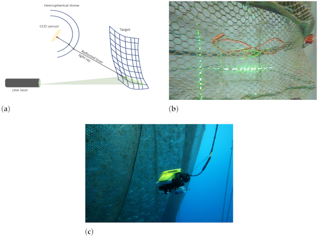
To estimate the relative posture to a mesh-like target the adopted approach is to fit the LVS measurements to a 3-D surface and then deduce the relative posture to the surface, as shown in Figure 6. In the current work, we will fit the LVS measurements from at least two line lasers target reflections to a 3-D plane.

Assume a line laser ℓ hits a target that is in front of the ROV camera sensor. The light reflection from the target produces a number of highlighted pixels $\left(n_{\ell }\right)$ on the image-plane, giving a matrix ${\mathbf{P}}^{\ell }$ of dimensions $n_{\ell }\times 2$. Each of the line lasers used for the LVS system can potentially give a number of points (when it hits any target) that lay on a known plane (according to the position of the lasers). Therefore, the ${\mathbf{P}}^{\ell }$ matrix contains the pixel coordinates of the $n_l$ pixels. Then, from Equation (21) and with a slight abuse of notation we have that ${\mathcal{T}}_{\ell }\left({\mathbf{P}}^{\ell }\right)={\mathbf{P}}_{w,\ell }^{S^{\prime }}$ are the 3-D positions of the laser reflections of the target on the CCD sensor in $<S^{\prime }>$. Note that the lasers are set up in such a way that the produced laser planes are non-coplanar, i.e., ${\mathbf{n}}_i^{S^{\prime }}\times {\mathbf{n}}_j^{S^{\prime }}\ne 0,\forall i\ne j$ in order to avoid ill-conditioning issues. Given $k\ge 2$ non-co-planar line lasers ${\ell }_1,\dots {\ell }_k$ we can produce the augmented matrix:

$${\mathbf{P}}_w^{S^{\prime }}=\left[\begin{array}{c}{\mathbf{P}}_{w,{\ell }_1}^{S^{\prime }}\\ ⋮\\ {\mathbf{P}}_{w,{\ell }_k}^{S^{\prime }}\end{array}\right].$$

(22)

Since the target fitted plane cannot physically pass from the origin, the plane equation in the $<S^{\prime }>$ frame can be written as:

$${\mathbf{r}}^{S^{\prime }}·\frac{{\widehat{\mathbf{n}}}_p^{S^{\prime }}}{d^{S^{\prime }}}=1$$

(23)

where ${\mathbf{r}}^{S^{\prime }}$ is any vector connecting $<S^{\prime }>$ with a point on the target. Then,

$$\frac{{\widehat{\mathbf{n}}}_p^{S^{\prime }}}{d^{S^{\prime }}}={\left({\mathbf{P}}_w^{S^{\prime }}\right)}^{†}\left[\begin{array}{c}1\\ ⋮\\ 1\end{array}\right]$$

(24)

where ${\left({\mathbf{P}}_w^{S^{\prime }}\right)}^{†}$ is the left pseudo-inverse of ${\mathbf{P}}_w^{S^{\prime }}$ that is guaranteed to be non-singular as long as our lasers are non-co-planar and have non-co-linear target projections. From this, we can immediately extract the relative posture to the mesh-like target that comprises the plane’s normal ${\widehat{\mathbf{n}}}_p^{S^{\prime }}$ and the distance to the plane $d^{S^{\prime }}>0$, by noting that $∥{\widehat{\mathbf{n}}}_p^{S^{\prime }}∥=1$. Note that due to the planar symmetry assumption, only relative pitch and relative yaw can be determined, i.e., rotation of the ROV along the roll direction cannot be recovered.

Now, using the unit direction vectors ${\widehat{\mathit{x}}}_{S^{\prime }},{\widehat{\mathit{y}}}_{S^{\prime }},{\widehat{\mathit{z}}}_{S^{\prime }}$ of the coordinate system $<S^{\prime }>$, the relative pitch can be extracted by projecting the plane’s normal vector along the $y-z$ plane, as:

$${\theta }_{S^{\prime }}=\frac{\pi }{2}-acos\left[\frac{{\left({\widehat{\mathbf{n}}}_p^{S^{\prime }}\right)}^T·(\mathit{I}-{\widehat{\mathit{x}}}_{S^{\prime }}·{\widehat{\mathit{x}}}_{S^{\prime }}^T)·{\widehat{\mathit{z}}}_{S^{\prime }}}{∥{\left({\widehat{\mathbf{n}}}_p^{S^{\prime }}\right)}^T·(\mathit{I}-{\widehat{\mathit{x}}}_{S^{\prime }}·{\widehat{\mathit{x}}}_{S^{\prime }}^T)∥}\right]$$

(25)

and the relative yaw can be extracted by projecting the plane’s normal vector along the $y-x$ plane, as:

$${\psi }_{S^{\prime }}=\frac{\pi }{2}-acos\left[\frac{{\left({\widehat{\mathbf{n}}}_p^{S^{\prime }}\right)}^T·(\mathit{I}-{\widehat{\mathit{z}}}_{S^{\prime }}·{\widehat{\mathit{z}}}_{S^{\prime }}^T)·{\widehat{\mathit{x}}}_{S^{\prime }}}{∥{\left({\widehat{\mathbf{n}}}_p^{S^{\prime }}\right)}^T·(\mathit{I}-{\widehat{\mathit{z}}}_{S^{\prime }}·{\widehat{\mathit{z}}}_{S^{\prime }}^T)∥}\right].$$

(26)

3.3. Automatic Calibration

Underwater vehicles are often exposed to harsh conditions, i.e., seawater (salinity), sun, and overworked by pressure. For this reason, the components and the system require regular maintenance, such as cleaning and sealing tests after every operation. Maintenance procedures require regular disassembly of the LVS as well, which, in turn, requires re-calibration to ensure accurate readings. In this subsection, an automatic calibration procedure for the LVS is provided. Figure 7 shows the developed calibration box which is used for the LVS re-calibration procedure.

A coordinate system $<G>$ is defined for the box. The four box planes ((L)eft, (R)ight, (F)orward, (D)own) are defined as:

$${\mathbf{r}}_b·{\widehat{\mathbf{n}}}_b^G=d_b,b\in \left\{L,R,F,D\right\}.$$

(27)

The ROV is located in an initially unknown position ${\mathit{S}}^G$ and with an initially unknown orientation ${\mathit{R}}_S^G$ in the calibration box. A set of $n_p$ patterns are applied at known positions ${\mathcal{P}}_i^G$, $i\in \left\{1,\dots n_p\right\}$ in the box. Let $p_{{\mathcal{P}}_i}$ be the pixel corresponding to pattern i. Then, from the dome model we have:

$$\mathcal{D}\left(p_{{\mathcal{P}}_i}\right)\to ({\widehat{\mathbf{n}}}_{\mathcal{D}i}^{S^{\prime }},{\mathbf{p}}_{\mathcal{D}i}^{S^{\prime }}),i\in \left\{1,\dots n_p\right\}.$$

(28)

Hence, the line ${\mathit{l}}_i$ connecting point ${\mathbf{p}}_{\mathcal{D}i}^{S^{\prime }}$ with ${\mathcal{P}}_i$ is provided by:

$${\mathit{l}}_i\left(\lambda \right)={\mathbf{p}}_{\mathcal{D}i}^{S^{\prime }}+{\lambda }_i{\widehat{\mathbf{n}}}_{\mathcal{D}i}^{S^{\prime }},\lambda \ge 0.$$

(29)

The laser plane for laser ℓ in the $<S^{\prime }>$ coordinate system is provided by:

$${\mathbf{r}}_{\ell }{\widehat{\mathbf{n}}}_{\ell }^{S^{\prime }}=d_{\ell }^{S^{\prime }}.$$

(30)

The automatic laser calibration then consists of the procedure to determine the parameters ${\widehat{\mathbf{n}}}_{\ell }^{S^{\prime }}$ and $d_{\ell }^{S^{\prime }}$ of each laser ℓ. To achieve this, the ${\mathit{S}}^G$ and ${\mathit{R}}_S^G$ parameters have to be determined first. Thus, for each pattern the following equation is held:

$${\mathcal{P}}_i^G={\mathit{S}}^G+{\mathit{R}}_S^G({\mathbf{p}}_{{\mathcal{D}}_i}^{S^{\prime }}+{\lambda }_i{\widehat{\mathbf{n}}}_{{\mathcal{D}}_i}^{S^{\prime }}),i\in \left\{1,\dots n_p\right\}.$$

(31)

Since the rotation matrix, ${\mathit{R}}_S^G$ is a function of three Euler angles, the above equations form a system of $3n_p$ equations with $n_p+6$ unknowns. This implies that at least 3 patterns are needed to solve the problem. However additional patterns will increase the accuracy of the calibration, also removing ambiguity issues. Hence, a cost function is formed:

$$V({\mathit{S}}^G,{\mathit{R}}_S^G,{\lambda }_1,\dots {\lambda }_{n_p})=\sum _{i=1}^{n_p}{∥-{\mathcal{P}}_i^G+{\mathit{S}}^G+{\mathit{R}}_S^G(p_{{\mathcal{D}}_i}^{S^{\prime }}+{\lambda }_i{\widehat{\mathbf{n}}}_{{\mathcal{D}}_i}^{S^{\prime }})∥}^2$$

(32)

where the ${\mathit{S}}^G,{\mathit{R}}_S^G,{\lambda }_1,\dots {\lambda }_{n_p}$ can be determined by the solution of the nonlinear minimization problem:

$$({\mathit{S}}^G,{\mathit{R}}_S^G,{\lambda }_1,\dots {\lambda }_{n_p})=argmin\left\{V({\mathit{S}}^G,{\mathit{R}}_S^G,{\lambda }_1,\dots {\lambda }_{n_p})\right\}.$$

(33)

The next step requires the projection of each laser on at least two separate box planes (it is sufficient that the projected line on the two planes is different). From ${\mathit{S}}^G,{\mathit{R}}_S^G$ that were calculated in the previous step, and using the plane equations, for each reflected target point $j_b$ from plane $\mathit{b}$, we have:

$$({\mathit{S}}^G+{\mathit{R}}_S^G({\mathbf{p}}_{{\mathcal{D}}_{j_b}}^{S^{\prime }}+{\lambda }_{j_b}{\widehat{\mathbf{n}}}_{{\mathcal{D}}_{j_b}}^{S^{\prime }})·{\widehat{\mathbf{n}}}_b^G=d_b.$$

(34)

However, since by construction $d_{\ell }\ne 0$, ${\lambda }_{j_b}$ should also satisfy:

$$({\mathbf{p}}_{{\mathcal{D}}_{j_b}}^{S^{\prime }}+{\lambda }_{j_b}{\widehat{\mathbf{n}}}_{{\mathcal{D}}_{j_b}}^{S^{\prime }})·\frac{{\widehat{\mathbf{n}}}_{\ell }^{S^{\prime }}}{d_{\ell }^{S^{\prime }}}=1.$$

(35)

Therefore, by solving the Equation (34) for ${\lambda }_{j_b}$ and substituting all ${\lambda }_{j_b}$’s in Equation (35), we can write each result as a row of the matrix $\mathbf{Y}$. Then:

$$\frac{{\widehat{\mathbf{n}}}_{\ell }^{S^{\prime }}}{d_{\ell }^{S^{\prime }}}={\mathbf{Y}}^{†}\left[\begin{array}{c}1\\ ⋮\\ 1\end{array}\right]$$

(36)

where ${\mathbf{Y}}^{†}$ is the left pseudo-inverse of $\mathit{Y}$ where the laser calibration parameters (${\widehat{\mathbf{n}}}_{\ell }^{S^{\prime }}$ and $d_{\ell }^{S^{\prime }}$) can be extracted by noting that $∥{\widehat{\mathbf{n}}}_{\ell }^{S^{\prime }}∥=1$.

4. A Filter for Mesh-like Structures

4.1. Preliminaries

In this section, a spatial filter is developed to discriminate mesh-like structures from other artifacts in the LVS measurements. This is useful in the case that the relative posture is sought with respect to mesh-like structures such as fishnets, Figure 6, where the LVS should be able to discern the difference between fishnet, fish, and air bubble reflections. The aim of the proposed filter is to only allow reflections from the mesh-like spatial structure that is being observed as a target. Additionally, note the additional (faint) reflections from the water tank surface to the water tank wall. Spatial filtering using the Fourier transformation has been reported for the identification of fabric structures in images in [29]. In our approach, we exploit the point cloud produced by the LVS in the $<S^{\prime }>$ coordinate system. We assume that multi-path reflections (e.g., light beams that reflect on the water surface and then hit a target) either do not exist or that they are weaker than single path reflections. This assumption is valid since was observed during the lab and sea experiments. Now observing that all LVS measurements (excluding multi-path reflections) are co-planar, i.e., they reside in the laser plane, a binary image containing the laser-plane reflections which is co-planar with the laser-plane can be created. Thus, an appropriate filter can be developed to discern between reflections that belong to the mesh-like structure and ones that do not.

4.2. Approach

Mesh-like structures have the characteristic of being periodic in 2-dimensions. Intersecting such structures with a straight line yields intersection points that appear with predetermined regularity. Depending on the mesh geometry, a maximum and a minimum distance can be derived for the intersection points as we traverse the intersecting line. Thus, the distance between consecutive intersections will lie between a maximum and a minimum range. This observation is applicable for almost all positions of the intersecting line. Singular (i.e., in the sense that such an occurrence has zero probability when randomly placing the intersecting line) positions occur only when the intersecting line is collinear with edges on the target. Assuming a laser plane hitting such a target, we can define a minimum and a maximum distance between consecutive reflections from the target in the 3D space, irrespective of the target’s orientation. In the development of the filter, reflections from target features that are collinear with the laser line will be ignored, as such features are considered to be either singularities or non-mesh-like targets. For example, in Figure 8a the maximum distance between consecutive reflections is the diameter of the hexagon and the minimum distance is the side of the hexagon. In Figure 8b, the maximum distance is the diagonal of the rectangle and the minimum distance is half the diagonal. Hence, every reflection from such targets will always fall between the minimum and the maximum period with one of its neighboring reflections.

4.2.1. Laser Plane Image

The first step is to create the binary image of the LVS reflections in the laser plane. To perform this, a rotation of the point cloud $p_w^{S^{\prime }}$ that lies on the laser plane, to the $x-y$ plane is performed. First let us fix an ortho-canonical coordinate system $<\ell >$ on the laser plane, with direction unit vectors expressed in the $<S^{\prime }>$ frame as ${\mathit{e}}_{x,\ell },{\mathit{e}}_{y,\ell },{\mathit{e}}_{z,\ell }$:

Let

$${\mathit{e}}_{z,\ell }={\widehat{\mathbf{n}}}_{\ell }^{S^{\prime }}.$$

Then,

$${\mathit{e}}_{y,\ell }=\frac{{\mathit{e}}_{y,S^{\prime }}\left(\mathit{I}-{\mathit{e}}_{z,\ell }{\mathit{e}}_{z,\ell }^T\right)}{∥{\mathit{e}}_{y,S^{\prime }}\left(\mathit{I}-{\mathit{e}}_{z,\ell }{\mathit{e}}_{z,\ell }^T\right)∥}$$

(37)

where ${\mathit{e}}_{y,S^{\prime }}$ is the y-direction in the $<S^{\prime }>$ frame (forward laser looking direction) and,

$${\mathit{e}}_{y,\ell }={\mathit{e}}_{z,\ell }\times {\mathit{e}}_{x,\ell }.$$

(38)

Now create the rotation matrix from frame $<\ell >$ to frame $<S^{\prime }>$ as:

$${\mathit{R}}_{\ell }^{S^{\prime }}={\left[{\mathit{e}}_{x,\ell }⋮{\mathit{e}}_{y,\ell }⋮{\mathit{e}}_{z,\ell }\right]}^T.$$

(39)

Then, the 3-D positions of the laser reflections ${\mathbf{P}}_w^{S^{\prime }}$ can be translated and rotated to fall in the $x-y$ plane of $<S^{\prime }>$ as follows:

$${\mathbf{p}}_{w,i}^{S^{\prime },S^{\prime }}={\mathit{R}}_{\ell }^{S^{\prime }}({\mathbf{p}}_{w,i}^{S^{\prime }}-{\mathit{e}}_{z,\ell }·d_{\ell }^{S^{\prime }}).$$

(40)

Note that the z-component of ${\mathbf{p}}_{w,i}^{S^{\prime },S^{\prime }}$ is zero, and ${\mathbf{P}}_w^{S^{\prime },S^{\prime }}$ is a 2D point-cloud. Hence, ${\mathbf{P}}_w^{S^{\prime },S^{\prime }}$ can be represented with a binary image.

Define $q_i^x\triangleq {\mathbf{p}}_{w,i}^{S^{\prime },S^{\prime }}·{\left[100\right]}^T$ and $q_i^y\triangleq {\mathbf{p}}_{w,i}^{S^{\prime },S^{\prime }}·{\left[010\right]}^T$. Let $x_L={min}_i{q}_i^x$, $x_R={max}_i{q}_i^x$, $y_U={max}_i{q}_i^y$, $y_D={min}_i{q}_i^y$ represent the four boundaries of the laser plane. Let $dx$, $dy$ represent the spatial discretization of the binary image (this depends primarily on the characteristics of the target—i.e., thread diameter, assuming the LVS has adequate resolution).

Assume a grid with discretization $dx$, $dy$ with $n_x=\lceil \frac{x_R-x_L}{dx}\rceil$ columns and $n_y=\lceil \frac{y_U-y_D}{dy}\rceil$ rows. Create an array of index sets $S_{idx}$ as follows:

$$S_{idx}(m,n)=\left\{i\left|m·dx\le q_i^x-x_L<m·dx+1\wedge n·dy\le q_i^y-y_L<n·dy+1\right.\right\}.$$

(41)

The binary image is then defined as follows:

$$Im(m,n)=\left\{\begin{array}{cc}1& \left|S_{idx}(m,n)\right|>0\\ 0& \left|S_{idx}(m,n)\right|=0\end{array}\right.$$

(42)

where $|·|$ denotes the set cardinality.

4.2.2. Binary Image Processing Filter

The aim of the proposed filter is to identify points that belong to the mesh-like structure. Let $d_{\theta }$ be the thread diameter of the mesh-like structure. Let $r_{min}$ be the minimum distance between consecutive threads (center-to-center) as these are intersected in the laser plane and $r_{max}$ the corresponding maximum distance. Then, a reflection from a target thread will have a size of $r{d}_{\theta }=\frac{d_{\theta }}{cos{\theta }_{lt}}$ where ${\theta }_{lt}$ the angle between the laser plane and the target thread. The choice of ${\theta }_{lt}$ should be such that $r{d}_{\theta }<r_{max}$, otherwise the target periodicity assumption will not be valid. In practice, we want to have $r{d}_{\theta }<<r_{min}$, which is achievable for typical mesh-like targets assuming appropriate configuration of the laser-plane roll angle. The starting elements of the filter (see Figure 9) can be constructed by defining three regions via three concentric circles: Region A with diameter $r{d}_{\theta }$, region B with radius $r_{min}-\frac{r{d}_{\theta }}{2}$ that excludes region A, and region C with radius $r_{max}+\frac{r{d}_{\theta }}{2}$ that excludes regions B and A.

Regions A, B and C define three binary valued structuring elements $St{r}_A$, $St{r}_B$ and $St{r}_C$, with the same discretization as the binary image, that are 1 in their respective regions and 0 outside.

We can now start defining our filtering algorithm. The binary image $Im$ is padded with ${\rho }_{pad}=\lceil r_{max}+\frac{r{d}_{\theta }}{2}\rceil$ cells to obtain the image $I{m}^{\prime }$. To determine the morphological operations the required limits have to be established.

Assume now that we have a laser reflection from the center of a thread of a mesh-like target centered at the $m,n$ pixel of $I{m}^{\prime }$ and the $St{r}_A$ is placed at that location, i.e., $St{r}_A(m,n)$. Considering the grid discretization, and assuming $dx=dy=dd$ the thread reflection will encompass at most $d{g}_{\theta }=\lceil \frac{r{d}_{\theta }}{dd}\rceil +1$ grid cells and this is the maximum number of cells that they are expected to be active in $I{m}^{\prime }\cap St{r}_A(m,n)$. Then, $I{m}^{\prime }\cap St{r}_B(m,n)$ will be empty and $I{m}^{\prime }\cap St{r}_C(m,n)$ will contain at most $2d{g}_{\theta }$ cells.

Assume now that we have a laser reflection from the edge of a thread of a mesh-like target centered at the $m,n$ pixel of $I{m}^{\prime }$ and we place $St{r}_A$ at that location. Then, only from $\lceil \frac{d{g}_{\theta }}{2}\rceil$ up to $d{g}_{\theta }$ cells will be active in $I{m}^{\prime }\cap St{r}_A(m,n)$. In $I{m}^{\prime }\cap St{r}_B(m,n)$ we can have at most $\lceil \frac{d{g}_{\theta }}{2}\rceil$ cells active, and in $I{m}^{\prime }\cap St{r}_C(m,n)$ will contain at least $\lceil \frac{3d{g}_{\theta }}{2}\rceil +1$ cells active.

Almost all reflections (excluding singularities) from the mesh-like target will fall within the ranges provided above. A new binary image $I{m}^{″}$ can now be created that only contains pixels that belong to the mesh-like structure. The set of actual points that correspond to the mesh-like structure can be recovered by feeding into $S_{idx}(m,n)$ the pixels of $I{m}^{″}$ that are active. The filtering algorithm provided by Algorithm 1, returns the 3-D positions of the laser reflections only from the mesh-like structure, ${\mathbf{P}}_w^{S^{*}}$.

Algorithm 1 Mesh filter algorithm

Require:$I{m}^{\prime }$, $St{r}_A$, $St{r}_B$, $St{r}_C$

Ensure: Mesh Reflections from mesh-like structure

1: loop $(m,n)\in \left\{1\dots n_x\times 1\dots n_y\right\}$

2:  $(m^{\prime },n^{\prime })$←$(m+{\rho }_{pad},n+{\rho }_{pad})$

3:  if $\lceil \frac{d{g}_{\theta }}{2}\rceil \le \left|I{m}^{\prime }\cap St{r}_A(m^{\prime },n^{\prime })\right|\le d{g}_{\theta }$ then

4:    if $0\le \left|I{m}^{\prime }\cap St{r}_B(m^{\prime },n^{\prime })\right|\le d{g}_{\theta }-\left|I{m}^{\prime }\cap St{r}_A(m^{\prime },n^{\prime })\right|$ then

5:     if $\lceil \frac{3d{g}_{\theta }}{2}\rceil \le \left|I{m}^{\prime }\cap St{r}_C(m^{\prime },n^{\prime })\right|\le 2d{g}_{\theta }$ then

6:        $I{m}^{″}(m,n)$← 1

7:     end if

8:    end if

9:  end if

10: end loop

11: k← 1

12: loop$(m,n)\in \left\{1\dots n_x\times 1\dots n_y\right\}$

13:   if $I{m}^{″}(m,n)$ then

14:     $Idx$←$S_{idx}(m,n)$,

15:     L←$\left|Idx\right|$

16:     loop$j\in \left\{1\dots L\right\}$

17:     ${\mathbf{P}}_{w,k}^{S^{*}}$←$p_{w,j}^{S^{\prime }}$

18:     k←$k+1$

19:     end loop

20:  end if

21: end loop

22: return ${\mathbf{P}}_w^{S^{*}}$

5. Experiments

5.1. Experimental Setup

In this section, the experimental setup for the system and the experimental results obtained during the performance evaluation of the system are presented. The validity of the proposed system is verified both in a laboratory-controlled environment setting Figure 10, as well as in real conditions at an offshore aquaculture installation Figure 11.

A Videoray Pro IV (ROV) was used for the experiments. The robot is equipped with a CCD camera, a Tilt Compensated Compass (TCC) sensor capable of providing roll, pitch, and yaw measurements, the LVS that was analyzed in this work, and a custom-developed control station. Furthermore, the robot was retrofitted with an inertial measurement unit (IMU) providing its acceleration and angular rates. The default ROV camera resolution is 720 × 576p with a frame-rate of 25 fps. The system software was developed in C/C++, using the Robotic Operating System (ROS) [30] and OpenCV [28] on a 12.04 Ubuntu Linux OS. The PC that was used for the experiments was an Intel i7, a dual-core laptop, with 8GB RAM memory. The ROV is powered by a boat-mounted generator through a tether whereas the laser system is powered by a dedicated battery.

5.2. Experimental Evaluation of the Mesh Filter Algorithm

In this section, the experimental validation of the methodology that is proposed in Section 4 is presented. In Figure 12a, a mesh-like target as seen from the ROV camera is depicted, while Figure 12b depicts the corresponding thresholded image. Using the hemispherical dome model that was developed in Section 2, the laser point clouds are extracted. The point cloud corresponding to the horizontal laser is depicted in Figure 13.

As can be seen from Figure 13, the laser point cloud contains reflections from the mesh-like structure, the water tank floor, and walls, as well as from the solid (non-mesh) object. From Figure 13, we can distinguish the different reflections from the laser point cloud. Considering only the horizontal laser line for this experiment, the reflections from the water tank floor can be easily recognized and eliminated because they are beyond the limits of the operational range zone. Note that the operational range zone is between 300 mm and 1000 mm since beyond this range the accuracy provided by the camera (pixels/cm${}^2$ on the target) and, more importantly, the laser beam scattering, cause the algorithm to fail since the laser (thin) plane assumption is no longer valid. The operational range can be improved using better laser optics for the same medium and camera analysis. Hence, reflections that appear beyond these limits, are not taken into account in the mesh filter algorithm. In the operational range, the algorithm should be able to detect the mesh-like structure and eliminate other artifacts.

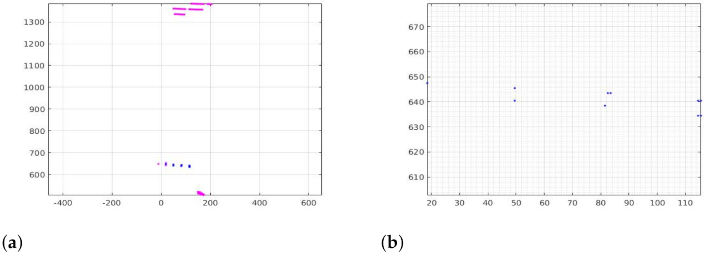
In order to identify which of the laser points belong to the mesh-like target, the Mesh Filter algorithm (Algorithm 1) was used. The mesh-like structure (mesh-target) used in the experiment has the following parameters: $d_{\theta }=2$ mm, $r{d}_{\theta }=10$ mm, $dd=1$ mm, $r_{min}=15$ mm, $r_{max}=35$ mm.

Figure 14 depicts the result after applying the Mesh Filter algorithm. As can be seen, the algorithm has rejected all reflections that did not belong to the mesh-like structure enabling the identification of the target.

5.3. Experimental Evaluation of the LVS in the Laboratory

Two series of tests were performed in a controlled environment in order to evaluate the performance of the LVS system in the laboratory. The tests validated the performance of the LVS system for linear distance and angular measurements from a static target in front of the ROV. The first series of experiments included positioning and aligning the ROV at specific positions in the water tank and comparing the LVS measurements against the known posture of the ROV. The ROV was aligned perpendicular to the water tank wall and was mounted underwater at 374 mm, 438 mm, 525 mm, and 659 mm from the wall. At each position, an array of measurements was performed to determine the distance $d^{S^{\prime }}$ reported by the LVS. Figure 15 depicts the distance error percentage in the distance reported by the LVS. As can be seen, the LVS accuracy is within $2.3\%$ of the measured distance.

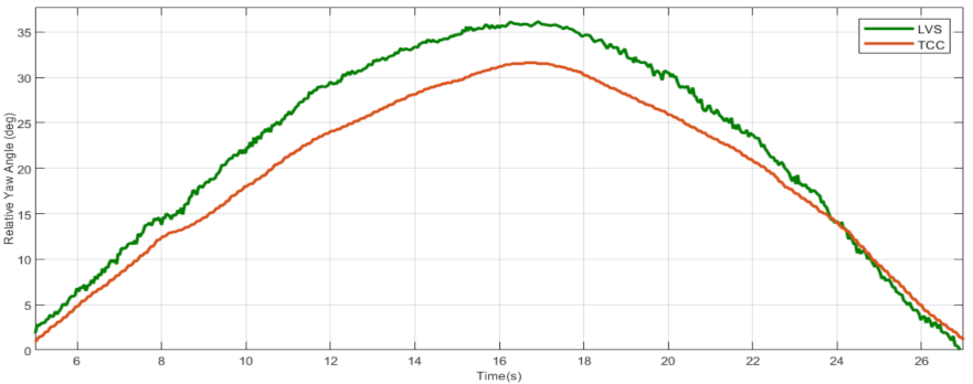
The second series of experiments included positioning the ROV at a constant distance from the water tank wall and changing the pitch and then the yaw angle of the ROV. The obtained measurements were compared against the relative orientation obtained through the TCC sensor. The results are depicted in Figure 16 for the relative pitch validation experiment and in Figure 17 for the relative yaw validation experiment.

As can be seen from both experiments the orientation error is within $14\%$ of the orientation reported by the TCC sensor. The main source of error in the experiments was caused by the scattering of the line laser beam in the transverse to the laser plane direction. This can be rectified by appropriately tuning the focus of the line laser beams or using better laser line optics.

5.4. LVS-Effect of Dome Model

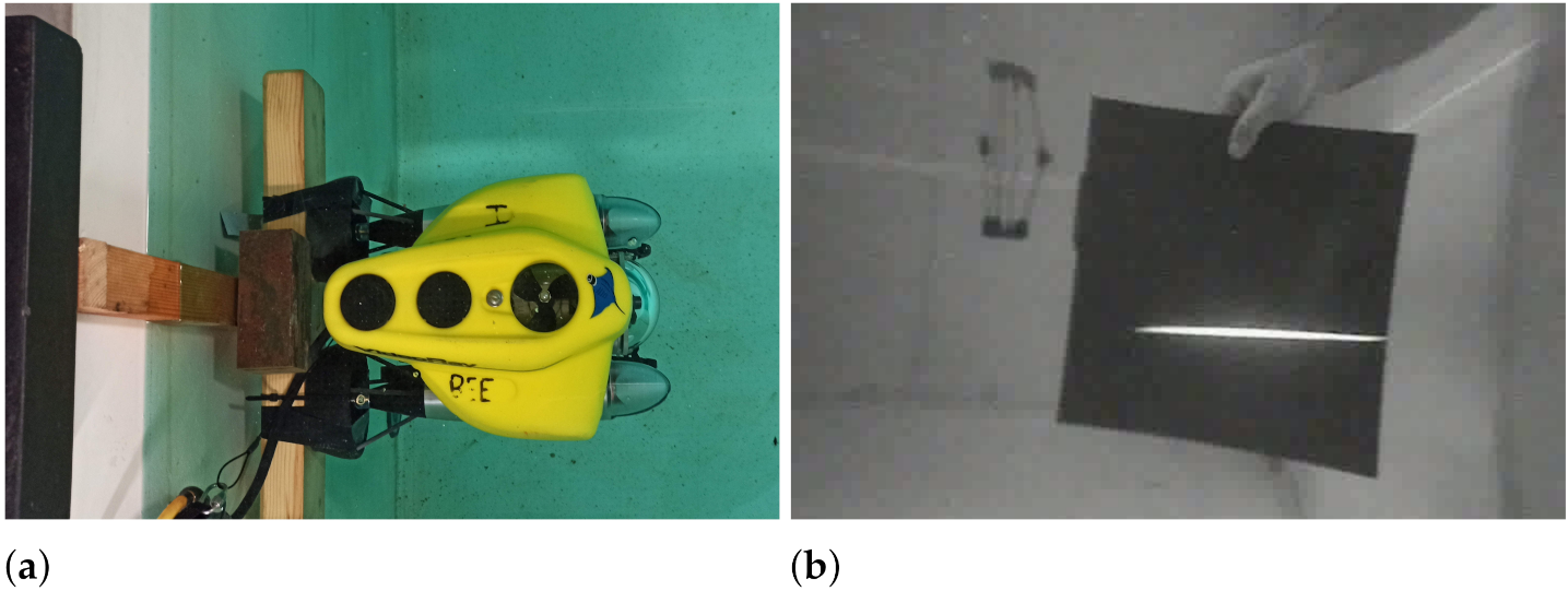
In order to demonstrate the effect of using the dome model that has been developed in this work, Section 2, in contrast to not using it for laser measurements, an experiment was devised and performed in the controlled laboratory environment. In particular, the ROV was mounted in the water tank and a moving target was placed in various predefined range positions from 300 mm to 1250 mm. The measurements were taken at increments of 100 mm, from 300 mm to 1200 mm, and then at decrements of 100 mm from 1250 mm to 350 mm, thus having points of measurement every 50 mm along the range. Figure 18 shows the setup and an image of the target as seen from the ROV dome camera.

The experiment was performed using the central horizontal laser. For each image, three points on the laser line image were considered; the leftmost, the central, and the rightmost. Each of the three points was used to calculate the distance by (a) using the dome model and (b) without using the dome model. Figure 19 shows a comparison of the measurements with (Dome) and without (No Dome) the dome model from the leftmost point (L) and the three-point average (Av).

More specifically, Figure 19 shows the measurements for leftmost and the three-point average, comparing in each plot the measurements taken with and without the use of the dome model. The actual range distance is also plotted for comparison. The best line fit (linear regression) is plot through the points of each measurement. It is shown that the dome model measurements are almost a perfect match to the plotted actual range distances. The measurements taken without the dome model are shown to have an increasing error as the range distance increases, with a deviation of over 300 mm at the 1250 mm range.

Figure 20 shows the percentage errors corresponding to Figure 19 measurements. For the errors, the line fit was used to eliminate random errors of target placement during the experiment and demonstrate the improvements due to the use of the dome model. Both plots show the use of the dome model to have an approximate increase in accuracy by a factor of 5. The plots show a higher accuracy at the left side of the laser, possibly suggesting minor deregulation of the laser mounting during the experiment since the error along the laser line for the whole range of 300 mm to 1250 mm is below $5.3\%$ (max at 300 mm range).

5.5. Testing the LVS System at an Offshore Aquaculture Installation

The LVS system was tested at an offshore aquaculture installation (https://youtu.be/BfyOdJnzkkA accessed on 15 November 2021). The preliminary test described below aimed at identifying the various operation features and parameters required for using the LVS system for inspecting aquaculture fishnets in actual field scenarios. Figure 21 shows images of aquaculture fishnets in offshore conditions, as captured from the ROV dome camera while using the LVS system.

In order to inspect the fishnet, a downward (depth increase) motion was performed, while at the same time keeping an approximately constant distance to the fishnet as well as a constant heading (https://youtu.be/HN669_R-Gmk accessed on 21 November 2021). The motion and measurements of the LVS equipped ROV is shown in Figure 22 below. The first subplot shows the depth of the ROV as given by the pressure sensor. The second subplot shows the range of the target as given by the LVS system. This is the shorter distance from the center of the dome to the target fitted plane. The third sub-plot shows the readings from the tilt-compensated compass (heading) and the target yaw angle as calculated by the LVS system. This is the yaw angle of the target fitted plane with respect to the ROV body.

In Figure 22, it is obvious that there is some correlation between the heading and the target yaw angle as expected. When the ROV yaws in a rightward direction, its heading increases. At the same time, an ideal stationary flat plane target would be perceived by the LVS system as rotating leftwards, thus increasing its yaw angle. However, in offshore aquaculture applications, the target is far from ideal, with a number of factors that affect the LVS system output. Those factors include:

• Shape of fishnet wall is not a flat surface;
• Shape of fishnet wall is not the same around the fish cage. Mooring and fishnet stitching and support alter the shape that would ideally be circular;
• Fishnet shape dynamically changes with sea currents. Folds and wavy surface features could develop on the fishnet surface during operation as can be seen in Figure 21a;
• Fishnet shape obtains altered by marine growth due to surface deposits altering shape, and weight of marine growth on net and mooring lines pulling unevenly at both static and dynamic current direction conditions;
• ROV position being altered by sea currents, forcing control manoeuvres to keep the required position.

Taking into account the above factors, Figure 22 shows the LVS system giving a clear indication of the range to the target surface. In combination with the target yaw angle also from the LVS system, they can be used to have a controlled motion for inspecting the fishnet surface.

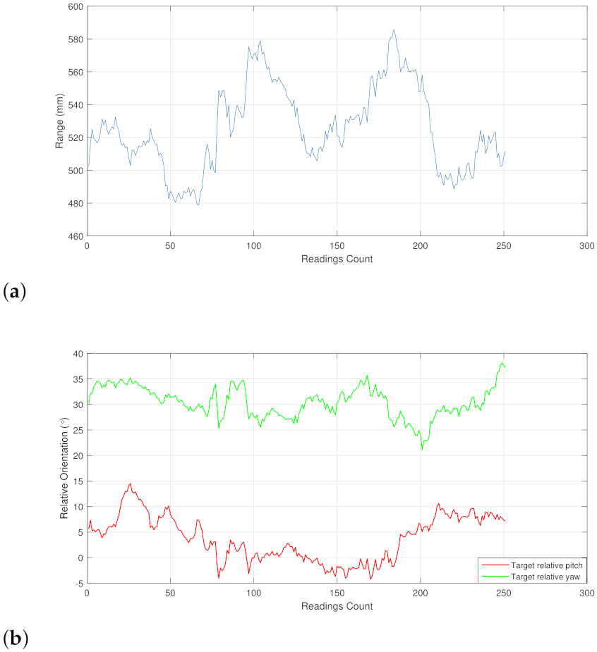
Figure 23 provides additional experimental results from a different portion of the fishnet, during the field experiments demonstrated in Figure 11 and Figure 24a. In this experiment, we chose to evaluate the performance of the LVS by implementing a PID controller on the ROV to stabilize its distance and yaw angle with respect to the fishnet using the LVS as feedback. Note that the ROV pitch (and roll) angles are passively stable and non-actuated. Some correlations between the results are expected as discussed and analyzed in the previous results.

In addition, operating close to a non-flat target created coupling effects, e.g., as the yaw increased the laser reflected to a further curved portion of the net resulting in reduced range (minimum distance from target fitted plane) measurement, while also having parasitic effects on the pitch. This effect can be reduced by aiming the lasers closer to the center of the camera’s field of view. However, this will negatively affect the ROV operators’ field of view.

6. Conclusions

The work presented, details the development and experimental validation of algorithms for a novel laser vision system (LVS) for measuring an ROV’s posture with respect to both solid and mesh-like targets in underwater environments. An analytical model for three-medium refraction (air, acrylic, water) that takes into account the nonlinear hemispherical optics was developed. The system development was motivated by the need for underwater ROV localization in close proximity to aquaculture fishnets, and due to the analytic nature of the solution, it is applicable to operation to mediums with varying refractive index, extending its applicable range. The LVS is capable of generating information as point cloud sets from each laser and, by utilizing the proposed algorithms, high-level information like distance and relative orientation of the target with respect to the ROV can be recovered. Due to the regular maintenance required by the system (typical for underwater vehicles and their components), an automatic calibration technique was developed. Furthermore, a spatial filter was developed and demonstrated, in order to discriminate the mesh-like targets from other artifacts in the LVS measurements. The algorithms developed in this work are appropriate for online operation.

Experimental results both in the laboratory and field experiments at an offshore aquaculture installation demonstrate the performance of the system. The analytical dome model significantly increases the calibration accuracy for the underwater camera-dome models as it turns out from the experimental results in Section 5.4. During field experiments, the proposed system demonstrated the expected performance that was recorded during laboratory testing, while the limitations of the system’s performance when operating near the water surface during intense sunlight Figure 24b and when operating in an environment with increased biomass were recorded. More specifically, due to algae growth and increased scattering due to higher biomass concentration in the proximity of the fishnet as can be seen in Figure 21 and Figure 24a, the mesh-like structure assumption was not valid on those portions of the fishnet and, hence, the mesh filter algorithm was not applicable there and also in cases where strong currents cause folding of the fishnet. Those scenarios will be considered in future works.

Further development of this work is towards an adaptive version of the proposed mesh filter that will be able to give estimation on variable biomass growth levels, appropriately adapting the thread diameter $d_{\theta }$ and other filter parameters. In addition, research towards utilizing the developed localization system to close the feedback loop in motion task planning strategies is being considered, for autonomous underwater structure inspection and maintenance tasks for operations that include but are not limited to aquaculture fishnet fault detection and repair.

References

- Yuh, J. Design and control of autonomous underwater robots: A survey. Auton. Robot. 2000, 8, 7–24. [Google Scholar] [CrossRef]
- Whitcomb, L.L. Underwater robotics: Out of the research laboratory and into the field. In Proceedings of the 2000 ICRA, Millennium Conference, IEEE International Conference on Robotics and Automation, Symposia Proceedings, San Francisco, CA, USA, 24–28 April 2000; Volume 1, pp. 709–716. [Google Scholar]
- Bogue, R. Underwater robots: A review of technologies and applications. Ind. Robot. Int. J. 2015, 42, 186–191. [Google Scholar] [CrossRef]
- Constantinou, C.C.; Loizou, S.G.; Georgiades, G.P.; Potyagaylo, S.; Skarlatos, D. Adaptive calibration of an underwater robot vision system based on hemispherical optics. In Proceedings of the Autonomous Underwater Vehicles (AUV), 2014 IEEE/OES, Oxford, MS, USA, 6–9 October 2014; pp. 1–5. [Google Scholar]
- Constantinou, C.C.; Loizou, S.G.; Georgiades, G.P. An underwater laser vision system for relative 3-D posture estimation to mesh-like targets. In Proceedings of the 2016 IEEE/RSJ International Conference on Intelligent Robots and Systems (IROS), Daejeon, Korea, 9–14 October 2016; pp. 2036–2041. [Google Scholar]
- Tsai, R.Y. A versatile camera calibration technique for high-accuracy 3D machine vision metrology using off-the-shelf TV cameras and lenses. IEEE J. Robot. Autom. 1987, 3, 323–344. [Google Scholar] [CrossRef] [Green Version]
- Heikkila, J.; Silvén, O. A four-step camera calibration procedure with implicit image correction. In Proceedings of the IEEE Computer Society Conference on Computer Vision and Pattern Recognition, San Juan, PR, USA, 17–19 June 1997; pp. 1106–1112. [Google Scholar]
- Treibitz, T.; Schechner, Y.Y.; Kunz, C.; Singh, H. Flat refractive geometry. IEEE Trans. Pattern Anal. Mach. Intell. 2012, 34, 51–65. [Google Scholar] [CrossRef] [PubMed] [Green Version]
- Jordt-Sedlazeck, A.; Koch, R. Refractive calibration of underwater cameras. Comput. Vis. ECCV 2012, 7576, 846–859. [Google Scholar]
- Kunz, C.; Singh, H. Hemispherical refraction and camera calibration in underwater vision. In Proceedings of the OCEANS 2008, Quebec City, QC, Canada, 15–18 September 2008; pp. 1–7. [Google Scholar]
- Castillón, M.; Palomer, A.; Forest, J.; Ridao, P. State of the Art of Underwater Active Optical 3D Scanners. Sensors 2019, 19, 5161. [Google Scholar] [CrossRef] [PubMed] [Green Version]
- Ribo, M.; Brandner, M. State of the art on vision-based structured light systems for 3D measurements. In Proceedings of the International Workshop on Robotic Sensors: Robotic and Sensor Environments, Ottawa, ON, Canada, 30 September–1 October 2005; pp. 2–6. [Google Scholar]
- Roman, C.; Inglis, G.; Rutter, J. Application of structured light imaging for high resolution mapping of underwater archaeological sites. In Proceedings of the OCEANS 2010, Sydney, NSW, Australia, 24–27 May 2010; pp. 1–9. [Google Scholar]
- Czajewski, W.; Sluzek, A. Development of a laser-based vision system for an underwater vehicle. In Proceedings of the International Symposium on Industrial Electronics, ISIE’99, Bled, Slovenia, 12–16 July 1999; Volume 1, pp. 173–177. [Google Scholar]
- Karras, G.C.; Panagou, D.J.; Kyriakopoulos, K.J. Target-referenced localization of an underwater vehicle using a laser-based vision system. In Proceedings of the OCEANS 2006, Boston, MA, USA, 18–21 September 2006; pp. 1–6. [Google Scholar]
- Wang, C.; Shyue, S.; Hsu, H.; Sue, J.; Huang, T. CCD camera calibration for underwater laser scanning system. In Proceedings of the OCEANS 2001, MTS/IEEE Conference and Exhibition, Honolulu, HI, USA, 5–8 November 2001; Volume 4, pp. 2511–2517. [Google Scholar]
- Cain, C.; Leonessa, A. Laser based rangefinder for underwater applications. In Proceedings of the American Control Conference (ACC), Montreal, QC, Canada, 27–29 June 2012; pp. 6190–6195. [Google Scholar]
- Hansen, N.; Nielsen, M.C.; Christensen, D.J.; Blanke, M. Short-Range Sensor for Underwater Robot Navigation using Line-lasers and Vision. IFAC-PapersOnLine 2015, 48, 113–120. [Google Scholar] [CrossRef] [Green Version]
- Lopes, F.; Silva, H.; Almeida, J.M.; Martins, A.; Silva, E. Structured light system for underwater inspection operations. In Proceedings of the OCEANS 2015, Genova, Italy, 18–21 May 2015; pp. 1–6. [Google Scholar]
- Muljowidodo, K.; Rasyid, M.A.; SaptoAdi, N.; Budiyono, A. Vision based distance measurement system using single laser pointer design for underwater vehicle. Indian J. Mar. Sci. 2009, 38, 324–331. [Google Scholar]
- Bleier, M.; Nüchter, A. Low-Cost 3D Laser Scanning in Air Orwater Using Self-Calibrating Structured Light. Int. Arch. Photogramm. Remote Sens. Spat. Inf. Sci. 2017, 42, 105. [Google Scholar] [CrossRef] [Green Version]
- Matos, G.; Buschinelli, P.; Pinto, T. Underwater Laser Triangulation Sensor Model with Flat Refractive Interfaces. IEEE J. Ocean. Eng. 2020, 45, 937–945. [Google Scholar] [CrossRef]
- Palomer, A.; Ridao, P.; Forest, J.; Ribas, D. Underwater laser scanner: Ray-based model and calibration. IEEE/ASME Trans. Mechatronics 2019, 24, 1986–1997. [Google Scholar] [CrossRef]
- Chantler, M.J.; Clark, J.; Umasuthan, M. Calibration and operation of an underwater laser triangulation sensor: The varying baseline problem. Opt. Eng. 1997, 36, 2604–2611. [Google Scholar] [CrossRef]
- AQUABOT. 2018. Available online: www.aquaculturebot.com (accessed on 10 May 2018).
- Lourakis, M.I. A brief description of the Levenberg-Marquardt algorithm implemented by levmar. Found. Res. Technol. 2005, 4, 1–6. [Google Scholar]
- Wozniak, B.; Dera, J. Light Absorption in Sea Water; Springer: New York, NY, USA, 2007; Volume 33. [Google Scholar]
- Bradski, G.; Kaehler, A. Learning OpenCV: Computer Vision with the OpenCV Library; O’Reilly Media, Inc.: Sebastopol, CA, USA, 2008; ISBN 9780596516130. [Google Scholar]
- Xu, B. Identifying fabric structures with fast Fourier transform techniques. Text. Res. J. 1996, 66, 496–506. [Google Scholar]
- Quigley, M.; Faust, J.; Foote, T.; Leibs, J. ROS: An open-source Robot Operating System. ICRA Workshop Open Source Softw. 2009, 3, 5. Available online: www.ros.org (accessed on 10 September 2021).
Figure 1.
Design and integration of the LVS on the Videoay Pro-4 platform. (a) CAD Model of ROV; (b) Integrated System with Laser Vision System.
Figure 2.
Geometric setup of the hemispherical refraction problem. The angles are exaggerated for demonstration purposes.
Figure 3.
The measured distance from the ROV to the chessboard is taken from the center of the dome .
Figure 4.
Chessboard patterns at know locations for the calibration of the dome model.
Figure 5.
The refractive index is calculated by the attached target in the field of view of the ROV’s camera.
Figure 6.
Using a line-laser based LVS to determine the relative posture to a mesh-like target. (a) Mesh-like target; (b) Fishnet structure; (c) Aquaculture fishnet.
Figure 7.
Calibration box for the LVS. (a) Lasers Calibration Box as seen by the ROV camera; (b) ROV with Laser Vision System.
Figure 8.
Mesh-like geometries: (a) hexagonal mesh and (b) diamond mesh.
Figure 9.
Structuring element regions.
Figure 10.
Laboratory mock-up experiment.
Figure 11.
Offshore aquaculture installations experiment. (a) The ROV operates an inspection task at aquaculture installation; (b) Aquaculture inspection operation by the proposed system.
Figure 12.
Mesh-like target. (a) Mesh-like target as seen by the ROV camera; (b) Thresholded Image.
Figure 13.
Laser point-cloud data (only for the horizontal laser).
Figure 14.
Mesh filter algorithm’s results. (a) The pink points denote all the reflections while the blue points indicate the mesh like structure points after the algorithm has been applied; (b) Mesh-like structure points. Notice the mm separation of the same point target reflection, caused due to the scattering of the laser beam e.g., at (50 mm, 643 mm).
Figure 15.
Distance error percentage versus the actual distance to the target.
Figure 16.
Relative pitch validation experiment in the laboratory water tank. The green line denotes the measurements of the LVS while the orange line is the measurement from TCC.
Figure 17.
Relative yaw validation experiment in the laboratory water tank. The green line denotes the measurements of the LVS while the orange line is the measurement from TCC.
Figure 18.
Experimental setup. (a) ROV mounted on the water tank wall; (b) Moving target as it seems from ROV camera.
Figure 19.
Measurements with and without the dome model. (a) Left laser points; (b) Average laser points.
Figure 20.
Measurement percentage error.
Figure 21.
Fishnet images of ROV using the LVS system.
Figure 22.
Relative yaw from the ROV to the target (fishnet) at sea.
Figure 23.
Experimental results of the LVS at an offshore aquaculture installation. (a) Minimum distance to fitted plane; (b) Relative yaw and pitch angles to fitted plane.
Figure 24.
Experimental evaluation at an offshore aquaculture installation. (a) The mesh filter algorithm was not applicable to some portions of the fishnet; (b) The LVS was not applicable under intense sunlight.