
Dimensional Synthesis of a Novel 3-URU Translational Manipulator Implemented through a Novel Method


LaMaViP, Department of Engineering, University of Ferrara, 44121 Ferrara, Italy
Robotics 2022, 11(1), 10; https://doi.org/10.3390/robotics11010010
Submission received: 19 November 2021
/
Revised: 12 December 2021
/
Accepted: 29 December 2021
/
Published: 5 January 2022
(This article belongs to the Special Issue Kinematics and Robot Design IV, KaRD2021)
Abstract
:A dimensional synthesis of parallel manipulators (PMs) consists of determining the values of the geometric parameters that affect the platform motion so that a useful workspace with assigned sizes can be suitably located in a free-from-singularity region of its operational space. The main goal of this preliminary dimensioning is to keep the PM far enough from singularities to avoid high internal loads in the links and guarantee a good positioning precision (i.e., for getting good kinematic performances). This paper presents a novel method for the dimensional synthesis of translational PMs (TPMs) and applies it to a TPM previously proposed by the author. The proposed method, which is based on Jacobians’ properties, exploits the fact that TPM parallel Jacobians are block diagonal matrices to overcome typical drawbacks of indices based on Jacobian properties. The proposed method can be also applied to all the lower-mobility PMs with block diagonal Jacobians that separate platform rotations from platform translations (e.g., parallel wrists).
1. Introduction
Designing the mechanical structure of a general-purpose machine, like a manipulator, has three mandatory steps that transform the original intuition of the designer into a real device: type synthesis [1,2,3,4], dimensional synthesis [1,2,4], and machine-element design [5,6,7]. The type synthesis identifies the most suitable topology (machine type) that can meet the motion requirements. The dimensional synthesis determines the values of the geometric parameters that affect the motion of the previously selected machine type. Eventually, the machine-element design determines the materials and actual sizes of the machine components that make them carry the nominal loads applied to the machine.
In the parallel-manipulator (PM) design, the dimensional synthesis [8,9,10] consists of determining the values of the above-mentioned geometric parameters (i.e., in this case, the ones that affect the platform motion) so that a useful workspace with assigned sizes can be located in a region of the operational space that is far from singularities. Indeed, satisfying this condition makes it possible to avoid high internal loads in the links and to guarantee a good positioning precision (i.e., to get good kinematic performances). This type of preliminary dimensioning is usually addressed [10,11,12,13] by using condition number [14,15,16] or manipulability [17] or transmission indices [18,19,20,21] as objective functions to optimize.
Condition number and manipulability, which are defined through the Jacobians appearing in the input–output instantaneous relationship (i.e., the linear mapping that analytically states a relationship between the actuated-joint rates (input) and the end-effector (platform) twist (output)), can identify the best performances at a given PM configuration (i.e., they are local indices) that are referable to this relationship. The duality between statics and kinematics makes these indices also carry pieces of information usually related to transmission indices [11,22,23]. Unfortunately, if the input and/or the output variables are not dimensionally homogeneous the proposed indices are not usable in their original form, since they refer to vector norms of the inputs and the outputs. Thus, in these cases, either some difficult-to-determine constants that homogenize the variables by taking into account the platform sizes must be included or some other analytic tricks must be conceived [11,16,24,25,26,27]. In addition, since, in general, these indices are not related to geometric or physics interpretations, even though they are able to identify configuration that are far from singularities, they are not able to quantify how far they are, which makes them difficult to use in a design context.
Transmission indices are extensions of the transmission/pressure angles of linkages [28,29]. Such extensions are based on the concept of virtual coefficient [30], which is defined as the virtual power delivered by a unit transmission wrench (transmission wrench screw (TWS)) on the corresponding unit output twist (output twist screw (OTS)) of the output link. They are defined as the ratio of the configuration-dependent (local) virtual coefficient and its maximum value obtained when the TWS is (virtually) rotated about a suitable characteristic point placed on the TWS axis. This definition has the merit of providing dimensionless indices (i.e., there is no homogeneity issue) that are frame independent, and the drawback of depending on the choices both of the characteristic point and of the adopted procedure for computing the maximum virtual coefficient. Moreover, despite the many definitions and extensions [18,19,20,21], their actual meanings when used in a design optimization still need further investigations.
With reference to the input–output instantaneous relationship, singularities are manipulator configurations where the one-to-one correspondence between actuated-joint rates and platform twist fails. PMs’ singularities are mainly collected into three groups [31,32]: type-I (serial) singularities, where the actuated-joint rates are indeterminate even if the platform is locked, type-II (parallel) singularities, where the platform twist is indeterminate even if the actuated joints are locked, and type-III singularities, where both the actuated-joint rates and the platform twist are indeterminate. The farther is the manipulator configuration from singularities, the higher are its positioning precision and the reduction of the internal loads in its components.
In lower-mobility PMs (LPMs), constraint singularities [33] may be present among their type-II singularities. Such singularities occur in LPMs where the connectivity of the kinematic chains (limbs)1 that in parallel join the platform to the frame (base) is higher than the degrees of freedom (DOF) of the LPM. The platform can change its motion type when the LPM is at a constraint singularity. Translational PMs (TPMs) are LPMs where, out of constraint singularities, the platform can only translate with respect to the base; accordingly, at a constraint singularity, the platform of a TPM may rotate. Evaluating the kinetostatic performances of TPMs must take into account the possible presence of constraint singularities (also named rotation singularities [35] in TPMs). TPM performances have been evaluated by using about all the above-mentioned types of indices (see [36,37] for Refs.).
Here, a novel method for the dimensional synthesis of TPMs is presented and applied to a TPM previously proposed by this author [38]. The proposed method, which is based on Jacobians’ properties, exploits the fact that TPM parallel Jacobians are block diagonal matrices [35] to overcome typical drawbacks of indices based on Jacobian properties. In particular, the proposed method introduces three novel indices: two of them are dimensionless and have clear geometric and static meanings and the remaining third rates the quality of the load transmission from the actuators to the platform. Consequently, the proposed methodology does not have homogeneity issues and indices’ minimum values to adopt during design come easily out from simple static and geometric considerations. The proposed method can be also applied to all the lower-mobility PMs with block diagonal Jacobians that separate platform rotations from platform translations (e.g., parallel wrists).
2. Materials and Methods
The canonic form of the input–output instantaneous relationship of a non-redundant PM is [31]
in which A6×6 is the 6 × 6 Jacobian that multiplies the platform twist, , where is the velocity of a reference platform point and ω is platform’s angular velocity; whereas, B6×n is the 6 × n Jacobian that multiplies the n-tuple, , collecting all the actuated-joint rates, where n ≤ 6 is the number of PM’s DOF. Both the Jacobians depend on the PM configurations.
With reference to Equation (1), the PM configurations that make the determinant of A6×6 equal to zero (in formula: det(A6×6) = 0) are type-II (parallel) singularities. The PM configurations that make the rank of B6×n lower than n (in formula: rank(B6×n) ≤ n) are type-I (serial) singularities; whereas, those that simultaneously make det(A6×6) = 0 and rank(B6×n) ≤ n are type-III singularities. In LPMs (i.e., if n < 6), by using the Gauss–Jordan elimination [39], Equation (1) can always be transformed in the following canonic form
which, if the submatrix H(6–n)×(6–n) is not singular (i.e., if det(H(6–n)×(6–n)) ≠ 0), can be further reduced to the form
where (⋅)i×j and 0i×j denote, respectively, an i × j matrix and an i × j null matrix, ξn×1 is a n-tuple collecting a suitable selection of ’s entries, and ξ(6–n)×1 is a (6–n)-tuple collecting the remaining entries of .
The condition det(H(6–n)×(6–n)) = 0, which analytically forbids the transformation of system (2) into system (3), identifies configurations where ξ(6–n)×1 becomes indeterminate; whereas, the condition det(Vn×n) = 0 identifies configurations where ξn×1 becomes indeterminate. Both these two conditions identify LPM configurations where the platform locally either gains additional DOFs or, without gaining further DOFs, is not controllable by the limbs any longer (i.e., they are type-II singularities). In general, all the non-null submatrices appearing in Equations (2) and (3) depend on the manipulator configuration. Nevertheless, when the LPM constrains the platform motion to belong to one displacement subgroup (e.g., translational or spherical or planar, etc., motion type) of the displacement group [40,41], the submatrix F(6–n)×n is always a null matrix (in formula: F(6–n)×n = 0(6–n)×n). In this case, ξ(6–n)×1 collects ’s entries that are forbidden in the displacement subgroup the LPM refers to. Consequently, the condition det(H(6–n)× (6–n)) = 0 identifies constraint singularities, that is, LPM configurations where the platform instantaneous motion may change its type.
In TPMs (n = 3), Equation (3) becomes
which is a particular case of Equation (1), where the Jacobian A6×6 is a block diagonal matrix, and can be split into the two smaller subsystems
In addition, since the platform translates, TPM configurations can be identified through the position vector p = (x, y, z)T that collects the coordinates, measured in a Cartesian system fixed to the base, of the reference platform point the velocity refers to. Consequently, the entries of the matrices V3×3, G3×3, and H3×3 can be written as functions of and of the TPM’s geometric constants.
Let vi (hi), for i = 1, 2, 3, denote the tridimensional vector collecting the entries of the i-th row of V3×3 (H3×3) so that V3×3 = [v1, v2, v3]T (H3×3 = [h1, h2, h3]T), system (5a), and system (5b) can always be multiplied, respectively, by the diagonal matrices Dv and Dh defined as follows:
Such matrix products transform systems (5a) and (5b) into the equivalent form
where and are matrices whose entries are dimensionless and whose rows are unit vectors. With reference to systems (7a) and (7b), the TPM’s analytic conditions that identify its singularities are
Condition (8a) (condition (8b)) refers to type-II singularities that are (are not) constraint singularities and imposes the coplanarity of three unit vectors, that is, it is also a geometric condition; whereas, condition (8c) refers to type-I singularities.
From a static point of view, the fact that, out of constraint singularities, the unit vectors, , for i = 1, 2, 3, individuate directions around which the platform cannot rotate (see Equation (7b)) means that the platform’s constraints due to the limbs generate torques parallel to those directions. Analogously, when the actuated joints are locked, the right-hand side of Equation (7a) becomes a null vector (i.e., Equation (7a) becomes similar to Equation (7b)) and the unit vectors, , for i = 1, 2, 3, individuate directions along which, out of type-II singularities, the platform reference point cannot translate. Consequently, the platform’s constraints due to the limbs also generate forces parallel to those directions and with lines of action passing through the platform reference point. This conclusion implies that the generic entry, tij, of matrix somehow has the meaning of transmission coefficient between the axis of the j-th actuated joint and the line with the direction of that passes through the reference platform point.
The above reported considerations allow the use of the left-hand sides of Equation (8) as measures of the TPM’s kinetostatic performances at a given configuration by defining the following local performance indices:
Indeed, kh and kv are absolute values of mixed products of three unit vectors; consequently, they are dimensionless and range from 0 to 1 with 0 that identifies singular configurations and 1 that identifies the farthest-from-singular configurations. Differently, kg is not negative and its minimum value, 0, identifies type-I singularities; in general, it has not a maximum value and is not dimensionless. Anyway, it can be stated that the higher kg is the better the motion/force transmission is with the chosen limb types.
Accordingly, the dimensional synthesis of a TPM can be implemented by sizing it so that a given useful workspace can be located in a region of the operational space where kh, kv, and kg are higher than assigned minimum values, that is, where the following inequalities are satisfied:
3. Results
TPMs of the 3-URU type [35] feature three equal limbs constituted of two links, one adjacent to the base and the other to the platform, joined to one another through a revolute (R)-pair and to the platform or to the base through a universal (U)-joint, that is, they are of the URU type. Since each U-joint is constituted of two R-pairs with axes mutually perpendicular and with a common intersection point (points Ai and Bi in Figure 1b), an URU limb contains five R-pairs in series: two at the endings (one adjacent to the base and the other adjacent to the platform) and three intermediate. If, in each limb (see Figure 1), the axes of the two R-pairs at the endings are parallel to one another and the axes of the three intermediate R-pairs are all parallel and, of course, perpendicular to the axes of the two R-pairs at the endings, the platform is constrained to translate when it is out of the constraint singularities [35].
LaMaViP 3-URU (Figure 1) is a particular geometry of a TPM family recently presented in an international patent by the author (see Section 6 for Refs.). The peculiarities of this geometry are (see Figure 1):
- (i).
- the axes of the three R-pairs (one for each limb) adjacent to the base are mutually perpendicular and share a common intersection (point O in Figure 1);
- (ii).
- the axes of the three R-pairs (one for each limb) adjacent to the platform are mutually perpendicular and share a common intersection (point P in Figure 1);
- (iii).
- in each URU limb, the actuated R-pair is the one not adjacent to the base in the U-joint adjacent to the base, but the actuator is located on the base.
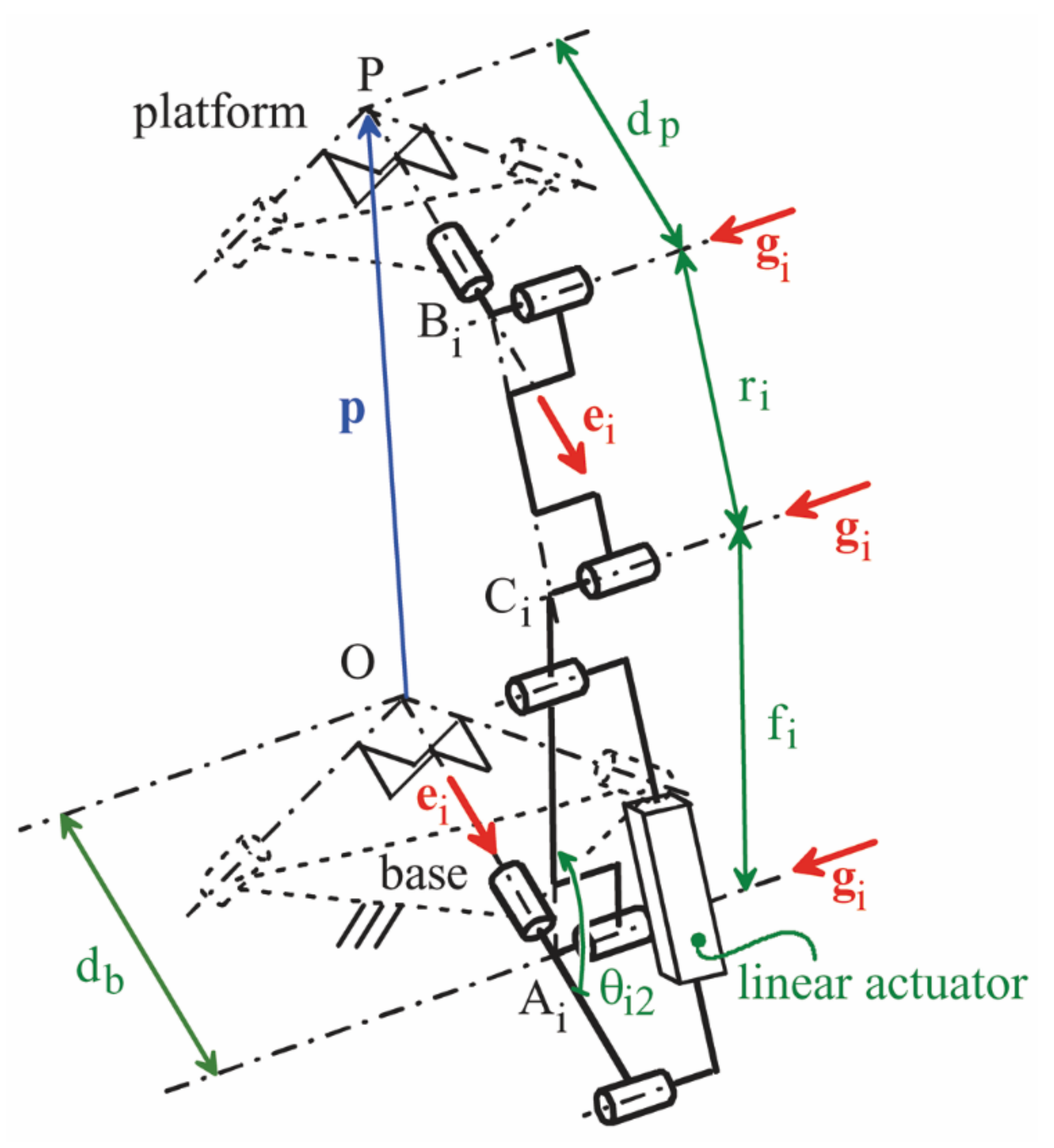
The singularity analysis of the LaMaViP 3-URU has been presented in [38] and its position analysis has been solved in [42]. With reference to Figure 1, the following notations are introduced: Oxbybzb (Pxpypzp) is a Cartesian reference fixed to the base (to the platform), and e1, e2, and e3 are unit vectors of the coordinate axes xb, yb, and zb (xp, yp, and zp), respectively, and, at the same time, unit vectors of the three R-pair axes fixed to the base (to the platform). Furthermore, Ai (Bi) for i = 1, 2, 3 are the centers of the U-joints adjacent to the base (to the platform). In the i-th limb, i = 1, 2, 3, without losing generality [43], the points Ai and Bi are assumed to lie on the same plane perpendicular to the axes of the three intermediate R-pairs; such a plane intersects at Ci the axis of the R-pair between the two U-joints. In addition, gi, i = 1, 2, 3, is the unit vector parallel to the axes of the three intermediate R-pairs of the i-th limb.
Moreover, the following definition/choices are introduced: dp = B1P = B2P = B3P; db = A1O = A2O = A3O; fi = AiCi; and ri = BiCi, for i = 1, 2, 3. In each URU limb, the five R-pairs are numbered with an index, j, that increases by moving from the base toward the platform; the actuated joint is the second R-pair. The angle θij, for i = 1, 2, 3, and j = 1,…, 5, is the joint variable of the j-th R-pair of the i-th limb; the actuated-joint variables are the angles θi2, i = 1, 2, 3 (see Figure 1). In addition, the phase reference of the angles θi1, i = 1, 2, 3, are given by the relationships (see Figure 1):
g1 = cosθ11 e2 + sinθ11 e3, g2 = −cosθ21 e1 + sinθ21 e3, g3 = cosθ31 e1 + sinθ31 e2
The introduced notations yield the following relationships (Figure 1):
where x, y, and z are the coordinates of the platform reference point (point P in Figure 1) measured in Oxbybzb, and
p = (P − O) = xe1 + ye2 + ze3
ai = (Ai − O) = dbei, bi = (Bi − O) = p + dpei, ci = (Ci − O) = ai + fiui, i = 1, 2, 3
With reference to Equations (5a) and (5b), this author demonstrated [38] that, for the LaMaViP 3-URU, the following relationships hold
which, since the vectors defined by Equation (11a) are unit vectors, bring one to conclude that Dv and Dh are both 3 × 3 identity matrices. As a consequence, for the LaMaViP 3-URU, , and the above-defined indices become (see Figure 1b)
3.1. Analytic Expression of the Indices
The geometric expressions of the indices given by Equation (12) can be transformed into functions of p as follows.
3.1.1. Index kh
The adopted notations bring one to write (see Figure 1b)
which, when introduced into the geometric definition (Equation (11a)) of hi, gives
Equation (13b), after the introduction of the analytic expression of p (i.e., p = xe1 + ye2 + ze3), becomes
whose introduction into Equation (12a) yields the sought-after expression, that is:
3.1.2. Index kv
The adopted notations (see Figure 1) bring the following relationships
which, after the introduction of the analytic expressions of p (i.e., p = xe1 + ye2 + ze3) and of hi (i.e., Equation (14)), become
with
which, when introduced into definition (12b), yield
with
(bi − ci) = ri vi = p + (dp − db) ei−fi (cosθi2 ei + sinθi2 hi) i = 1, 2, 3
b1 − c1 = [x + (dp − db) − f1 cosθ12]e1 + [1 − f1 m1 sinθ12] ye2 + [1 − f1 m1 sinθ12] ze3
b2 − c2 = [1 − f2 m2 sinθ22] xe1 + [y + (dp − db) − f2 cosθ22]e2 + [1 − f2 m2 sinθ22] ze3
b3 − c3 = [1 − f3 m3 sinθ32] xe1 + [1 − f3 m3 sinθ32] ye2 + [z + (dp − db) − f3 cosθ32]e3
n1 = [1 − f1 m1 sinθ12]; n2 = [1 − f2 m2 sinθ22]; n3 = [1 − f3 m3 sinθ32]
q1 = (dp − db) − f1 cosθ12; q2 = (dp − db) − f2 cosθ22 ; q3 = (dp − db) − f3 cosθ32
The actuated-joint variables, θ12, θ22, and θ32, can be eliminated from Equation (20) by using the solution formulas of the inverse position analysis presented in [44], that is:
where
and j might be limited to only one value according to the limb configuration selected when assembling the TPM.
3.1.3. Index kg
The analysis of Figure 1b reveals that the closed polyline OPBiCiAiO always lies on a plane (i.e., it is a polygon) that is perpendicular to the unit vector gi. As a consequence, the following geometric relationships can be written
which gives
whose introduction into Equation (12c) yields
3.2. Simulation Results
The values assumed by the indices kh, kv, and kg in the free-from-singularity regions of the operational space have been computed as a preliminary computation to identify in the operational space where conditions (10) may be satisfied. Such computation is illustrated below.
3.2.1. Index kh
Expression (15) of kh shows that (see [38] for details) the three coordinate planes of reference Oxbybzb constitute the geometric locus of LaMaViP 3-URU’s constraint singularities. In addition, its analysis reveals that it does not contain the geometric constants of the studied TPM and that the change of sign of any coordinate does not affect the value of kh. The second observation brings the conclusion that the values assumed by kh have the same pattern in every octant of reference Oxbybzb; consequently, this analysis can be conducted in only one octant, hereafter the first octant is chosen.
Regarding the values of kh, when the condition x = y = z, which identifies the line whose points are equally distant from the coordinate planes and the coordinate axes (i.e., from the surfaces of the constraint-singularity locus), is introduced into Equation (15), the constant value is obtained for all the points of that line provided the point O is excluded. As it is confirmed below, this value is also the maximum value that kh can assume.
The circumferences centered at a generic point D = (d, d, d)T of the line x = y = z that lie on a plane perpendicular to that line (see Figure 2) have the following parametric equations
where r is the radius of the circumference, ψ is the parameter, and λ = r/d. The introduction of Equation (26) into Equation (15) yields
which is a function that depends only on λ and ψ. Figure 3 shows the diagram of this function. Since the two parameters λ and ψ uniquely identify all the lines of the considered octant that pass through O, this result proves that each line passing through O collects points that have a constant value of kh given by the diagram of Figure 3 provided that point O is excluded.
3.2.2. Index kv
Expression (19) of kv depends on the geometric constants of the studied TPM. Such constants are the following eight: db, dp = μdb with μ = dp/db, ri and fi = νiri with νi = fi/ri and i = 1, 2, 3. Since a well-sized TPM has equal limbs, hereafter, the analysis will be restricted to this case by introducing the following conditions on the geometric constants: r1 = r2 = r3 = ρ and ν1 = ν2 = ν3 = ν. This restriction reduces the geometric constants to four, that is, db, μ, ρ, and ν.
Figure 4 shows the values assumed by kv along the line x = y = z = −d, where d is the parameter of the line, for different values of ρ, μ, and ν when the limbs are all assembled so that the index j appearing in Equation (21) is equal to 0. The analysis of Figure 4 reveals that, for all the analyzed geometries, kv reaches its maximum value (i.e., kv = 1) in different positions along the line, that is, for different values, dmax, of the line parameter, d. In particular, dmax increases when ρ or μ or ν increase. In addition, Figure 4 highlights that the neighborhood, Δd, centered at dmax, in which kv keeps values adequately high (e.g., greater than 0.7), increases when ρ increases and, if ρ ≥ 3db, it is always wide enough for locating a useful workspace with sizes of industrial interest.
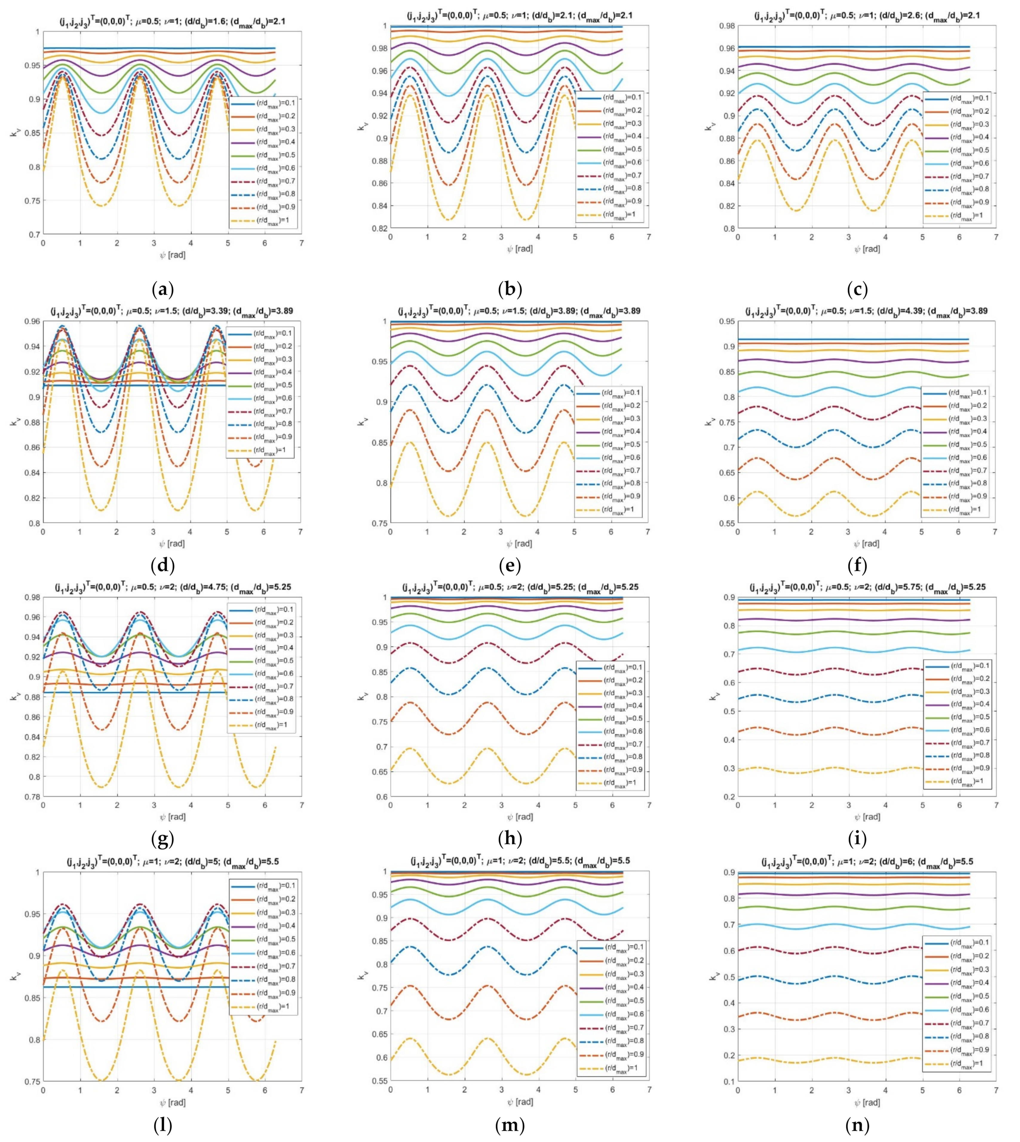
For the case ρ = 4db, Figure 5 shows the values of kv on circumferences (see Figure 2) with radius r, centered at point D’ = (−d, −d, −d)T of the line x = y = z, that lie on planes perpendicular to the same line. In particular, it refers to the four geometries of Figure 4 in the following three positions along the above-mentioned line: (d/db) = (dmax/db) − 0.5, (d/db) = (dmax/db), and (d/db) = (dmax/db) + 0.5. The analysis of Figure 5 reveals that, in all the geometries, if (r/dmax) ≤ 0.5, kv is always greater than 0.75 with values that are greater than 0.95 for (d/db) = (dmax/db) and greater than 0.86 for (d/db) = (dmax/db) − 0.5.
These results bring the conclusion that, in all the analyzed geometries, a useful workspace with the shape of a right circular cylinder having height equal to db and radius r ≤ 0.5dmax, if it is centered at D’max = (−dmax, −dmax, −dmax)T by keeping its axis along the line x = y = z, will guarantee a high value of kv everywhere inside it.
3.2.3. Index kg
Figure 2b highlights that the points O, Ai, Ci, Bi, and P lie on the same plane, which is perpendicular to the unit vector gi, and that the i-th limb, over moving together with this plane, which can rotate around the line passing through points O and Ai, performs a planar motion inside this plane. Figure 6 shows the i-th limb in this plane together with the force, Fivi, that the limb applies to the platform and the torque, Migi, the actuator applies in the actuated-joint. The moment of equilibrium about Ai of the i-th limb projected along gi gives the relationship Mi = Fisi where si is the arm of Fivi that can be expressed as follows (see Figure 6):
Equation (28) reveals that si is a “transmission coefficient” depending on θi3, which plays the role of a “transmission angle”. Such a transmission angle rates the quality of the transmission from the actuator to the platform in the i-th limb. Moreover, the comparison of Equation (28) with Equation (12c) provides the conclusion that kg is just the product of the transmission coefficients, si for i = 1, 2, 3, of the three limbs. This result concurs with the general interpretation given to kg in Section 2.
Since, in the studied TPM, the meaning of the tree factors whose product gives kg is clear, instead of assigning a lower limit to the whole kg (i.e., Equation (10)), a lower limit will be assigned to each factor. Such a limit can be deduced from the ample literature (see [45,46] for Refs.) on the transmission angles of planar linkages that suggest the imposition of the following limitations
which yield
Condition (30) must be checked in the whole useful workspace by using Equation (24) every time the link lengths ri and fi (i.e., in our particular case, ρ and ν) are chosen. If condition (30) is satisfied for the minimum, θi3,min, and the maximum, θi3,max, values of θi3, it will be satisfied in the whole useful workspace. With reference to Figure 6, the minimum (maximum) value of θi3 occurs when the length of the segment AiBi is maximum (minimum). The following relationships come out from Equation (24)
3.3. Functional Parameters Determination
A useful workspace with the shape of a right circular cylinder having height equal to db is chosen. The above-reported results show that such a workspace shape must be always located with its axis lying on the line x = y = z to get good kinetostatic performances; whereas, its position along that line and its radius must be selected by considering the chosen values of kh,min and kv,min. Eventually, when the position and the sizes of the cylinder have been completely determined, condition (30) must be verified.
kh (kv) is a mixed product of unit vectors related to the directions of three reaction moments (forces) equilibrating external loads applied to the platform. Consequently, a reasonable minimum value of kh (kv) is kh,min = 0.5 (kv,min = 0.5), which, in the worst case, implies a reaction moment (force) with a magnitude 1.5 times the magnitude of the external load. Figure 3 shows that the condition kh ≥ 0.5 is satisfied by choosing λ = (r/d) ≤ 0.6. Moreover, by choosing ρ = 4db, μ = 0.5, and ν = 1.5, Figure 5d–f2 shows that the condition kv ≥ 0.5 is always satisfied if (r/dmax) ≤ 0.7 where dmax = 3.89db. The conclusion is that, the choices ρ = 4db, μ = 0.5, and ν = 1.5 locate the right circular cylinder, used as a useful workspace, with its bases equally distant from point D’max = (−3.89db, −3.89db, −3.89db)T and choose its radius r = 0.6dmax = 2.334db (see Figure 7).
Now that the shape and the location of the useful workspace is completely defined, condition (30) must be verified. Figure 7 shows the two configurations of the i-th limb in which the segment AiBi reaches its minimum and maximum lengths. The data reported in Figure 7 make it possible to compute the following values: and . The introduction of these values into Equation (31) yields , which corresponds to , and , which corresponds to . Consequently, condition (30) is verified in the whole workspace with an ample safety margin and the transmission angles are always very good.
4. Discussion
The dimensional synthesis of the LaMaViP 3-URU clearly proves that the novel method proposed for evaluating TPMs’ kinetostatic performances is based on three indices whose meaning is easy to understand during the design of the machine. In particular, since two indices are dimensionless and have geometric and static meanings and the remaining third index refers to the quality of the load transmission from the actuators to the platform, the choice of their minimum values to satisfy inside the useful workspace comes out in a natural way from simple static and geometric considerations.
Moreover, it is worth noting that these indices provide a map of the possible design choices. Consequently, their use leaves the designer free to adopt the choices that better fit the technical requirements the machine has to satisfy.
The proposed methodology for TPMs’ dimensional synthesis, even though it is based on Jacobians, does not have homogeneity issues. Such a feature makes the proposed indices suitable for comparing the kinetostatic performances of different TPMs. A possible procedure for comparing different TPMs by using these indices is to consider the minimum, the maximum, and the average values of each index in the useful workspace since they are local indices.
The proposed method requires only that the input/output instantaneous relationship of the studied LPM can be put in a canonic form in which the parallel Jacobian (i.e., the one that multiplies the platform twist) is a block diagonal Jacobian that separates platform rotations from platform translations. Therefore, over TPMs, it is certainly applicable also to spherical PMs (parallel wrists) and extendable to Schoenflies (SCARA) PMs, planar PMs, and other LPMs that can satisfy this condition.
Regarding the dimensional synthesis of the LaMaViP 3-URU, the obtained geometry and useful workspace (Figure 7) are comparable to the ones of commercial delta robots (e.g., ABB IRB360). In addition, the found limb geometry with the link adjacent to the base that is 1.5 times longer than the one adjacent to the platform suggests that the actuated-joint variable, θi2, is controllable by simply introducing a linear actuator as shown in Figure 8. Such an actuation system is easy to manufacture and makes the limb stiff enough for using the LaMaViP 3-URU in CNC machine tools.
5. Conclusions
A novel method for the dimensional synthesis of lower-mobility PMs (LPMs) has been presented. The proposed method can be applied to all the translational PMs (TPMs) and, in general, to all the LPM types whose input/output instantaneous relationship can be put in a canonic form in which the parallel Jacobian is a block diagonal matrix that separates platform rotations from platform translations (e.g., parallel wrists).
The presented method is based on three indices, of which two are dimensionless and have clear geometric and static meanings and the remaining third rates the quality of the load transmission from the actuators to the platform. These features of the three indices make the proposed methodology not affected by homogeneity issues of the involved input/output variables. In addition, since the values of the indices are easy to relate to particular design requirements through their geometric and static meanings, the proposed technique is particularly useful for addressing the design of novel LPM architectures.
The application of the method to TPMs has been illustrated in depth and it is also illustrated by using it in the dimensional synthesis of the LaMaViP 3-URU, which is a novel TPM type recently proposed by the author. Such a synthesis has provided a clear map of the possible design choices used to determine a workspace and a machine geometry that are comparable to the ones of commercial delta robots and are suitable for industrial applications.
Future works will also present applications of the method to other types of LPMs and will try to extend the method to all non-redundant PMs. Regarding LaMaViP 3-URU, future works will address its machine-element design referring to industrial applications together with the evaluation of its dynamic performances.
6. Patents
Di Gregorio, R.: Meccanismo Parallelo Traslazionale. 23 March 2020; Italy Patent Application No. 102020000006100; published on 30 September 2021, as international PCT patent No.: WO2021/191054A1.
Funding
This research was funded by the University of Ferrara (UNIFE), FAR2020 and developed at the Laboratory of Mechatronics and Virtual Prototyping (LaMaViP), Department of Engineering, UNIFE.
Institutional Review Board Statement
Not applicable.
Informed Consent Statement
Not applicable.
Data Availability Statement
This work does not use experimental data. The data necessary to replicate the computations illustrated in the paper are included in the text of the paper.
Conflicts of Interest
The authors declare no conflict of interest. The funders had no role in the design of the study; in the collection, analyses, or interpretation of data; in the writing of the manuscript, or in the decision to publish the results.
References
- Hartenburg, R.S.; Denavit, J. Kinematic Synthesis of Linkages; McGraw-Hill: New York, NY, USA, 1964; ISBN 9780070269101. [Google Scholar]
- Tsai, L.W. Mechanism Design: Enumeration of Kinematic Structures According to Function; CRC Press LLC: Boca Raton, FL, USA, 2001. [Google Scholar]
- Kong, X.; Gosselin, C.M. Type Synthesis of Parallel Mechanisms; Springer: Berlin/Heidelberg, Germany, 2007; ISBN 978-3-642-09118-6. [Google Scholar]
- McCarthy, J.M.; Soh, G.S. Geometric Design of Linkages; Springer: Berlin/Heidelberg, Germany, 2011. [Google Scholar]
- Bhandari, V.B. Design of Machine Elements, 3rd ed.; Tata McGraw-Hill: New Delhi, India, 2010. [Google Scholar]
- Jiang, W. Analysis and Design of Machine Elements; Wiley: Singapore, 2019. [Google Scholar]
- Ashby, M.F. Materials Selection in Mechanical Design, 5th ed.; Butterworth-Heinemann: Burlington, MA, USA, 2016. [Google Scholar]
- Lou, Y.J.; Liu, G.F.; Li, Z.X. A general approach for optimal design of parallel manipulators. In Proceedings of the ICRA 2004, New Orleans, LA, USA, 26 April–1 May 2004. [Google Scholar]
- de-Juan, A.; Collard, J.-F.; Fisette, P.; Garcia, P.; Sancivrian, R. Multi-objective optimization of parallel manipulators. In New Trends in Mechanism Science, Mechanisms and Machine Science; Pisla, D., Ceccarelli, M., Husty, M., Corves, B., Eds.; Springer: Dordrecht, The Netherlands, 2010; Volume 5. [Google Scholar] [CrossRef]
- Angeles, J. Fundamentals of Robotic Mechanical Systems; Springer: Dordrecht, The Netherlands, 2014. [Google Scholar]
- Merlet, J.P. Jacobian, Manipulability, Condition Number, and Accuracy of Parallel Robots. ASME J. Mech. Des. 2006, 128, 199–206. [Google Scholar] [CrossRef]
- Patel, S.H.; Sobh, T. Manipulator Performance Measures—A Comprehensive Literature Survey. J. Intell. Robot. Syst. 2014, 77, 547–570. [Google Scholar] [CrossRef] [Green Version]
- Rosyid, A.; El-Khasawneh, B.; Alazzam, A. Review article: Performance measures of parallel kinematics manipulators. Mech. Sci. 2020, 11, 49–73. [Google Scholar] [CrossRef]
- Salisbury, J.K.; Craig, J.J. Articulated Hands: Force Control and Kinematic Issues. Int. J. Robot. Res. 1982, 1, 4–17. [Google Scholar] [CrossRef]
- Gosselin, C.; Angeles, J. A Global Performance Index for the Kinematic Optimization of Robotic Manipulators. J. Mech. Des. 1991, 113, 220–226. [Google Scholar] [CrossRef]
- Khan, W.A.; Angeles, J. The Kinetostatic Optimization of Robotic Manipulators: The Inverse and the Direct Problems. ASME J. Mech. Des. 2006, 128, 168–178. [Google Scholar] [CrossRef]
- Yoshikawa, T. Manipulability of Robotic Mechanisms. Int. J. Robot. Res. 1985, 4, 3–9. [Google Scholar] [CrossRef]
- Sutherland, G.; Roth, B. A transmission index for spatial mechanisms. ASME J. Eng. Ind. 1973, 95, 589–597. [Google Scholar] [CrossRef]
- Chen, C.; Angeles, J. Generalized transmission index and transmission quality for spatial linkages. Mech. Mach. Theory 2007, 42, 1225–1237. [Google Scholar] [CrossRef]
- Wang, J.; Wu, C.; Liu, X.J. Performance evaluation of parallel manipulators: Motion/force transmissibility and its index. Mech. Mach. Theory 2010, 45, 1462–1476. [Google Scholar] [CrossRef]
- Liu, H.; Huang, T.; Kecskeméthy, A.; Chetwynd, D.G. A generalized approach for computing the transmission index of parallel mechanisms. Mech. Mach. Theory 2014, 74, 245–256. [Google Scholar] [CrossRef] [Green Version]
- Chang, W.-T.; Lin, C.-C.; Lee, J.-J. Force Transmissibility Performance of Parallel Manipulators. J. Robot. Syst. 2003, 20, 659–670. [Google Scholar] [CrossRef]
- Kim, H.S.; Choi, Y.J. Forward/inverse force transmission capability analyses of fully parallel manipulators. IEEE Trans. Robot. Autom. 2001, 17, 526–531. [Google Scholar] [CrossRef]
- Ma, O.; Angeles, J. Optimum architecture design of platform manipulators. In Proceedings of the 5th International Conference on Advanced Robotics’ Robots in Unstructured Environments, Pisa, Italy, 19–22 June 1991; Volume 2, pp. 1130–1135. [Google Scholar] [CrossRef]
- Staffetti, E.; Bruyninckx, H.; De Schutter, J. On the Invariance of Manipulability Indices. In Advances in Robot Kinematics; Lenarčič, J., Thomas, F., Eds.; Springer: Dordrecht, The Netherlands, 2002. [Google Scholar] [CrossRef] [Green Version]
- Kim, S.-G.; Ryu, J. New dimensionally homogeneous Jacobian matrix formulation by three end-effector points for optimal design of parallel manipulators. IEEE Trans. Robot. Autom. 2003, 19, 731–736. [Google Scholar] [CrossRef]
- Cardou, P.; Bouchard, S.; Gosselin, C. Kinematic-Sensitivity Indices for Dimensionally Nonhomogeneous Jacobian Matrices. IEEE Trans. Robot. 2010, 26, 166–173. [Google Scholar] [CrossRef]
- Hain, K. Applied Kinematics; McGraw-Hill: New York, NY, USA, 1967. [Google Scholar]
- Dresner, T.L.; Buffinton, K.W. Definition of pressure and transmission angles applicable to multi-input mechanisms. ASME J. Mech. Des. 1991, 113, 495–499. [Google Scholar] [CrossRef]
- Ball, R.S. A Treatise on the Theory of Screws; Cambridge University Press: Cambridge, UK, 1900. [Google Scholar]
- Gosselin, C.M.; Angeles, J. Singularity analysis of closed-loop kinematic chains. IEEE Trans. Robot. Autom. 1990, 6, 281–290. [Google Scholar] [CrossRef]
- Zlatanov, D.; Fenton, R.G.; Benhabib, B. A unifying framework for classification and interpretation of mechanism singularities. ASME J. Mech. Des. 1995, 117, 566–572. [Google Scholar] [CrossRef]
- Zlatanov, D.; Bonev, I.A.; Gosselin, C.M. Constraint Singularities as C-Space Singularities. In Advances in Robot Kinematics: Theory and Applications; Lenarčič, J., Thomas, F., Eds.; Springer: Dordrecht, The Netherlands, 2002; pp. 183–192. [Google Scholar]
- Hunt, K.H. Kinematic Geometry of Mechanisms; Clarendon Press: Oxford, UK, 1990. [Google Scholar]
- Di Gregorio, R. A Review of the Literature on the Lower-Mobility Parallel Manipulators of 3-UPU or 3-URU Type. Robotics 2020, 9, 5. [Google Scholar] [CrossRef] [Green Version]
- Brinker, J.; Corves, B.; Takeda, Y. Kinematic and dynamic dimensional synthesis of extended Delta parallel robots. In IFToMM International Symposium on Robotics & Mechatronics (ISRM2017); Yang, R., Takeda, Y., Zhang, C., Fang, G., Eds.; Springer: Dordrecht, The Netherlands, 2017; pp. 131–143. [Google Scholar] [CrossRef]
- Brinker, J.; Corves, B.; Takeda, Y. Kinematic performance evaluation of high-speed Delta parallel robots based on motion/force transmission indices. Mech. Mach. Theory 2018, 125, 111–125. [Google Scholar] [CrossRef]
- Di Gregorio, R. A Novel 3-URU Architecture with Actuators on the Base: Kinematics and Singularity Analysis. Robotics 2020, 9, 60. [Google Scholar] [CrossRef]
- Meyer, C.D. Matrix Analysis and Applied Linear Algebra; SIAM: Philadelphia, PA, USA, 2000. [Google Scholar]
- Hervé, J.M. The Mathematical Group Structure of the Set of Displacements. Mech. Mach. Theory 1994, 29, 73–81. [Google Scholar] [CrossRef]
- Hervé, J.M. The Lie Group of Rigid Body Displacements, a Fundamental Tool for Mechanism Design. Mech. Mach. Theory 1999, 34, 719–730. [Google Scholar] [CrossRef]
- Di Gregorio, R. Direct Position Analysis of a Particular Translational 3-URU Manipulator. ASME J. Mech. Robot. 2021, 13, 061007. [Google Scholar] [CrossRef]
- Di Gregorio, R.; Parenti-Castelli, V. A Translational 3-DOF Parallel Manipulator. In Advances in Robot Kinematics: Analysis and Control; Lenarcic, J., Husty, M.L., Eds.; Kluwer: Norwell, MA, USA, 1998; pp. 49–58. [Google Scholar]
- Di Gregorio, R. Position Analysis of a Novel Translational 3-URU with Actuators on the Base. In New Advances in Mechanisms, Mechanical Transmissions and Robotics. MTM & Robotics 2020; Lovasz, E.C., Maniu, I., Doroftei, I., Ivanescu, M., Gruescu, C.-M., Eds.; Springer: Dordrecht, The Netherlands, 2020; pp. 80–90. [Google Scholar] [CrossRef]
- Balli, S.S.; Chand, S. Transmission angle in mechanisms (Triangle in mech). Mech. Mach. Theory 2002, 37, 175–195. [Google Scholar] [CrossRef]
- Pennestrì, E.; Valentini, P.P. A review of simple analytical methods for the kinematic synthesis of four-bar and slider-crank function generators for two and three prescribed finite positions. In Buletin Stiintific Seria Mecanica Aplicata; University of Pitesti: Pitesti, Romania, 2009; pp. 128–143. [Google Scholar] [CrossRef]
| 1 | According to [34], here, the term “limb connectivity” denotes the DOF number the platform would have if it were connected to the base only through that limb. |
| 2 | It is worth noting that Figure 5 holds only for the choice ρ = 4db, a different choice of ρ requires the determination of analogous diagrams through the above reported formulas. |
Figure 1.
LaMaViP 3-URU: (a) overall scheme and notations, (b) detailed scheme of the i-th limb (figure reproduced from [38]).
Figure 1.
LaMaViP 3-URU: (a) overall scheme and notations, (b) detailed scheme of the i-th limb (figure reproduced from [38]).

Figure 2.
An octant of Oxbybzb: (a) line x = y = z and plane passing through point D = (d,d,d)T perpendicular to that line, (b) top view along the line x = y = z containing the circumference, centered at D, with radius r, lying on the plane perpendicular to the line x = y = z.
Figure 2.
An octant of Oxbybzb: (a) line x = y = z and plane passing through point D = (d,d,d)T perpendicular to that line, (b) top view along the line x = y = z containing the circumference, centered at D, with radius r, lying on the plane perpendicular to the line x = y = z.

Figure 3.
Diagram of the function defined by Equation (27).

Figure 4.
Values of kv along the line x = y = z= −d for different values of ρ and limbs assembled so that the index j appearing in Equation (21) is equal to 0 in the cases: (a) μ = 0.5, ν = 1; (b) μ = 0.5, ν = 1.5; (c) μ = 0.5, ν = 2; (d) μ = 1, ν = 2.
Figure 4.
Values of kv along the line x = y = z= −d for different values of ρ and limbs assembled so that the index j appearing in Equation (21) is equal to 0 in the cases: (a) μ = 0.5, ν = 1; (b) μ = 0.5, ν = 1.5; (c) μ = 0.5, ν = 2; (d) μ = 1, ν = 2.

Figure 5.
Values of kv on circumferences (see Figure 2) with radius r, centered at point D’ = (−d, −d, −d)T of the line x = y = z, that lie on planes perpendicular to the same line, in the case ρ = 4db for (a,d,g,l) (d/db) = (dmax/db)−0.5, (b,e,h,m) (d/db) = (dmax/db), (c,f,i,n) (d/db) = (dmax/db) + 0.5, and the geometries (a,b,c) μ = 0.5, ν = 1, (d,e,f) μ = 0.5, ν = 1.5, (g,h,i) μ = 0.5, ν = 2, and (l,m,n) μ = 1, ν = 2.

Figure 6.
View of the i-th limb in the plane perpendicular to the unit vector gi represented together with the force Fivi it applies to the platform and the torque Migi applied by the actuator in the actuated joint.
Figure 6.
View of the i-th limb in the plane perpendicular to the unit vector gi represented together with the force Fivi it applies to the platform and the torque Migi applied by the actuator in the actuated joint.

Figure 7.
Cylindrical workspace: view of the i-th limb in the meridian plane passing through the line x = y = z and containing the coordinate axis of Oxbybzb that is parallel to the unit vector ei.
Figure 7.
Cylindrical workspace: view of the i-th limb in the meridian plane passing through the line x = y = z and containing the coordinate axis of Oxbybzb that is parallel to the unit vector ei.

Figure 8.
The i-th limb with a linear actuator that controls the actuated-joint variable θi2.

Publisher’s Note: MDPI stays neutral with regard to jurisdictional claims in published maps and institutional affiliations. |
© 2022 by the author. Licensee MDPI, Basel, Switzerland. This article is an open access article distributed under the terms and conditions of the Creative Commons Attribution (CC BY) license (https://creativecommons.org/licenses/by/4.0/).
Share and Cite
MDPI and ACS Style
Di Gregorio, R. Dimensional Synthesis of a Novel 3-URU Translational Manipulator Implemented through a Novel Method. Robotics 2022, 11, 10. https://doi.org/10.3390/robotics11010010
AMA Style
Di Gregorio R. Dimensional Synthesis of a Novel 3-URU Translational Manipulator Implemented through a Novel Method. Robotics. 2022; 11(1):10. https://doi.org/10.3390/robotics11010010
Chicago/Turabian StyleDi Gregorio, Raffaele. 2022. "Dimensional Synthesis of a Novel 3-URU Translational Manipulator Implemented through a Novel Method" Robotics 11, no. 1: 10. https://doi.org/10.3390/robotics11010010
Note that from the first issue of 2016, this journal uses article numbers instead of page numbers. See further details here.