
Infrastructure-Aided Localization and State Estimation for Autonomous Mobile Robots


1
Institute for Regulation and Control Systems, Karlsruhe Institute of Technology (KIT), 76131 Karlsruhe, Germany
2
Mechanical and Mechatronics Engineering Department, University of Waterloo, 200 University Ave W, Waterloo, ON N2L 3G1, Canada
3
Mechanical Engineering Department, University of Alberta, 9211-116 Street NW, Edmonton, AB T6G 1H9, Canada
*
Author to whom correspondence should be addressed.
Robotics 2022, 11(4), 82; https://doi.org/10.3390/robotics11040082
Submission received: 11 July 2022
/
Revised: 13 August 2022
/
Accepted: 16 August 2022
/
Published: 18 August 2022
(This article belongs to the Special Issue Advances in Industrial Robotics and Intelligent Systems)
Abstract
:A slip-aware localization framework is proposed for mobile robots experiencing wheel slip in dynamic environments. The framework fuses infrastructure-aided visual tracking data (via fisheye lenses) and proprioceptive sensory data from a skid-steer mobile robot to enhance accuracy and reduce variance of the estimated states. The slip-aware localization framework includes: the visual thread to detect and track the robot in the stereo image through computationally efficient 3D point cloud generation using a region of interest; and the ego motion thread which uses a slip-aware odometry mechanism to estimate the robot pose utilizing a motion model considering wheel slip. Covariance intersection is used to fuse the pose prediction (using proprioceptive data) and the visual thread, such that the updated estimate remains consistent. As confirmed by experiments on a skid-steer mobile robot, the designed localization framework addresses state estimation challenges for indoor/outdoor autonomous mobile robots which experience high-slip, uneven torque distribution at each wheel (by the motion planner), or occlusion when observed by an infrastructure-mounted camera. The proposed system is real-time capable and scalable to multiple robots and multiple environmental cameras.
1. Introduction
Navigating mobile robots in dynamic environments with human presence makes visual odometry challenging due to occlusion and dynamic features. This necessitates multi-modal (e.g., camera, LiDAR, inertial) data fusion to identify and remove the dynamic features for feature-based localization [1,2], address disturbance and model mismatch challenges for LiDAR based localization [3,4], or tackle perceptually degraded conditions through distributed estimation [5,6]. In this regard, multi-modal state estimation approaches for mobile robots [7,8] are revolutionizing accurate navigation for indoor applications (e.g., warehouse robotics or service robots using on-board sensors) where the loss of reception and low bandwidth of commercial Global Navigation Satellite Systems (GNSS), inhibit reliable robot state measurements.
One of main challenges for the the existing multi-modal state estimators that utilize on-board inertial measurement unit (IMU) data and visual odometry through monocular/stereo cameras is the wheel slip in the longitudinal and lateral directions. This is due to: (i) Model uncertainties caused by the wheel force saturation in the robot dynamical model (by various robot payloads, changing surface conditions, or harsh cornering scenarios) impacting estimation error and update frequency in real-time [9,10,11]; and (ii) The real-time performance of state estimators for safe motion planning and controls in a scene with dynamic features [12,13]. Infrastructure-aided state estimation approaches which leverage visual/radar data measured by fixed sensors and communication with the robot are proposed in the literature to deal with perceptually degraded conditions and dynamic features for navigation of mobile autonomous systems [14,15,16]. This is cost effective as it reduces the number of on-board sensors, specially for large-scale networked robotic systems. In [17], cameras installed on the ceiling detect multiple robots with unique markers and determine their position and heading states based on the distance to fixed markers on the ground and known marker sizes. A stationary fisheye camera installed on the ceiling is used in [14] for indoor robot localization, in which the pose is determined based on the azimuth and elevation of the line of view (to the center of the segmentation). Multiple fixed surveillance cameras are used in [18] to detect the robot and static objects to construct a 2D map. Pose data from low-cost cameras mounted on ceiling is fused with on-board LiDAR odometry data for robot state estimation in [19] where the fusion of camera and odometry is performed in a map with an adaptive Monte Carlo approach. The existing infrastructure-aided localization approaches require visual markers or free line of sight to the robot [17,19], heavily rely on robot model, and are challenged by occluded scenes and model uncertainties due to the wheel slip.
In order to compensate for the wheel longitudinal/lateral slip in robots with nonholonomic constraints, kinematic- or dynamic-based slip estimation/compensation methods have been adopted in the literature [20,21] using on-board sensory data. The dynamic-based approaches require wheel stiffness properties and vertical forces that may change due to various payloads and road surface conditions [22]. Kinematic-based methods, on the other hand, use wheel odometry and inertial data to estimate the slip with upper bounded mean square estimation error (MSE) through nonlinear or stochastic observers [12,23,24]. A high-gain observer is designed in [25] to deal with unknown model parameters. To avoid model complexities due to tire force nonlinearities (and the combined-slip effect), an empirical parameterized kinematic model is proposed in [26] for robot state estimation. An event-based Kalman observer is designed in [27] to fuse IMU data and wheel odometry for heading and speed estimation. However, the information from on-board state observers has not been used for fusion with infrastructure sensing units to enhance reliability of the pose estimation. In addition, the computational efficiency and accuracy are main challenges for the existing infrastructure-mounted visual tracking and localization methods that use low-cost wide-angle lenses.
To address computational time and accuracy challenges of the existing visual and kinematic/dynamic model based localization methods (to be executed on embedded systems and robot’s on-board processing units), this paper develops and experimentally verifies a cooperative state estimator using: (i) Proprioceptive data from low-cost odometry sensors of a skid-steer mobile robot; and (ii) Region of Interest (ROI)-based processing and visual tracking on the 3D point clouds obtained from fixed sensing units. The main contributions of the paper are summarized as:
- Design of a computationally efficient ROI-based pose estimator using 3D point clouds from a stationary stereo camera with a wide-angle (fisheye) lens.
- Developing an infrastructure-aided localization framework which is scalable for large systems with multiple robots using communication between a slip-aware onboard observer and the stationary sensing unit.
2. Background and System Overview
The localization framework includes visual tracking through forming an ROI for computationally enhanced processing at the edge (e.g., embedded Jetson Xavier) and a slip-aware state observer at the robot using proprioceptive data. The visual tracking is through a fixed low-cost stereo camera, Intel Realsense T265. As illustrated in Figure 1, the system has independent visual tracking thread and ego motion thread.
The state vector is defined by for the proposed framework, where the longitudinal position, lateral position, and heading of the robot in the reference fixed frame is denoted by x, y, and , respectively. The local robot body frame is denoted by , which is at the geometrical center of the robot and is depicted in Figure 2. The reference coordinate system is derived from at time zero .
The visual tracking thread estimates the robot pose based on the captured images of the stationary stereo camera in the environment. The occlusion cases, in which visual-based pose estimates are intermittent (or not available), will be addressed by the Covariance Intersection (CI) fusion with the estimated states from the slip-aware motion model. The updated pose by CI is then used as a corrected pose for the relative motion prediction in the next sample time. The robot pose is a time-varying transformation where the rotation matrix with is about the Z-axis of the , and the position vector with is the longitudinal and lateral robot position in the reference frame .
2.1. Visual Tracking Thread
The visual tracking thread includes frontend and backend modules as illustrated in Figure 3. The frontend performs image processing and object detection. In the image processing step, the stereo image pair is undistorted and rectified. The object detection generates a boundingbox for the robot within the rectified stereo images. The area in the images enclosed with the boundingbox is termed as region of interest. The undistorted and rectified images, and image coordinates of the corresponding bounding box are used in the backend to localize the robot using the 3D position of points on the robot.
With the assumption of the pinhole model and known extrinsic parameters, the constraints for the projection of point clouds in onto the two image planes are derived. These constraints are described with epipolar geometry, and determine the area in the image planes where the same point in is mapped on. Figure 4 illustrates the epipolar geometry for two non rectified images. The projection of the point m into the camera centers and defines the epipolar plane which intersects the image plane and forming epipoles and for the left/right images. The homogeneous transformation with the rotation matrix R and translation vector p between the camera centers describes the extrinsic parameters [28].
The position of a point in is determined with the intersection of the projection ray in 3D from the left and right image plane for the same mapped world point. The mapping of the x,y and z coordinate of a point from onto the left and right rectified image (Figure 5 and Figure 6) plane as is described as ( denotes the left and right sides, respectively) where and
are the extended camera matrix for the left and right image planes. The images have the same focal length in X and Y direction as well as the same principal point in Y direction; they are geometrically shifted with the baseline b in X direction. The radial distance r for perspective pinhole projection between the principal point and image coordinates of incoming ray of the point m is and the angle between the principal axis and the ray is . The radial fisheye distortion factor is modeled [29] as with the individual lens distortion parameter . The distorted image coordinates and are
which are then converted into undistorted image coordinates
Subsequent to this, a Yolov4 object detector [30] is used for 2D detection of the robot in the undistorted left image. The Yolov4 model is trained on a custom collected dataset of the robot for identification of the robot as a class label since the state-of-the-art COCO class labels have no training data corresponding to the robot.
Remark 1.
The output of the Yolov4 custom training detector at th step is a bounding box around the robot in the image yielding the extents of the box in the horizontal and vertical directions of the image. This enables an ROI which will be used to extract a frustum of the point cloud representing the robot. Point cloud processing will then be applied exclusively to the ROI-based frustum, i.e., interior . This bounding box-informed frustum significantly reduces the computational cost compared to processing the point cloud as a whole.
2.2. Point Cloud Computation and Post Processing
The feature extraction is restricted to the ROI, , and is scalable for visual tracking in multi-robot settings. The robot is depicted inside the ROI in the left and right image plane of the undistorted and rectified images. The aim is to find the image coordinates and v (in the left image) and (in the right image plane) of the world point m, as see in Figure 5 and Figure 6.
For feature extraction, ORB features [31,32] were used, where the extracted features are matched within the stereo image pair and between subsequent captured image pairs. It is assumed that the remaining image coordinates represent the same point on the robot platform, then, these points’ 3D coordinates are reconstructed. Based on the epipolar geometry, the depth is computed for each match with the horizontal image coordinates and of the left and right stereo image and the baseline b, as well as the focal length f of the camera, then the depth is used for and with the vertical image coordinate of the left stereo image plane as illustrated in Figure 7. The coordinates are computed for every match and transformed into . All points lead to a point cloud assumed to be derived from the surface of the robot. The point cloud is processed with the PCL library [33,34] and a statistical outlier filter. The filter rejects points that are further away from their neighbors compared to the average of the point cloud. The input parameters are the number of neighbors to calculate the average distance for a given point and a ratio to set the threshold based on the standard deviation across the point cloud.
The 2D projection of the point cloud is used to enhance the reliability of the 3D point clouds for navigating the robot far from the stationary sensing unit (i.e., the stereo visual node). The Euclidean center of the 2D points (which is less sensitive to outliers) is considered as an estimate of the position, i.e., at time step and will be corrected using the slip-aware motion model, which is described in the next section.
For orientation estimation, a linear regressor is used for a moving horizon of the estimated states. The angle between the estimated linear function and the world frame’s longitudinal axis is then considered as the orientation of the robot. To cope with situations when the robot is not driving or turning with zero radius, a plausibility check is applied. The plausibility check rejects estimates if the linear regression is too short or the distance between the position estimates and the line is greater than a threshold.
3. Infrastructure-Aided State Estimation
A kinematic model is introduced and parametrized to predict the motion in presence of wheel skidding and slipping. A covariance intersection (CI) method is then used to update the prediction.
3.1. Slip-Aware Motion Model
The autonomous mobile robot used to evaluate the localization approach is the skid-steer Clearpath’s Jackal robot, which is subject to the large wheel longitudinal slip in various cornering scenarios. The kinematic motion model in the following predicts the robot states using the heading and wheel rotational speed in the robot body frame . The robot’s motion is defined based on the instantaneous center of rotation (IC) as shown in Figure 8, assuming that the robot is a rigid body and has a planar motion with nonholonomic constraints.
The longitudinal velocity, lateral velocity, and yaw rate are denoted by , , and in the body frame and are expressed in terms of the left/right wheel rotational speeds as
where , the wheel rolling radius is denoted by , and includes the model parameter vector as follows
where is the instantaneous center of the front-left and rear-left tires of the robot and denotes the instantaneous center of the front-right and rear-right tires of the robot. In the schematic provided in Figure 8, due to nonholonomic constraints and since the longitudinal speed on the right side (i.e., rotational speed multiplied by the effective rolling radius ) is larger than the robot speed , the instantaneous center is located on the right side (i.e., in the body frame).
The instantaneous center is expressed in as , where [26]. The IC locations for the left and right wheels are expressed in as and , respectively. It is assumed that the longitudinal position of ICs along the x-axis lie all on a parallel line to the Y-axis, i.e., and have the same angular velocity. The lateral IC locations, which are bounded variables, are expressed as [21]:
where and are parameters accounting for model uncertainties (tire inflation and longitudinal slip ratios at each corner of the robot) and is the tire rolling radius. The location of IC is bounded, i.e., and even reached in the proximity of straight trajectories where the numerator and denominator in (6) are of the same infinitesimal order which leads to finite values for , .
The boundedness of need to be guaranteed for lateral stability and minimizing the robot’s sideslip angle in harsh turning. Using the transformation between and the world frame, the robot states in are expressed as
where is the robot heading and represents model uncertainties. Then, the parameter identification process consists of two steps: gathering representative data from on-board and infrastructure-mounted sensory data; and developing an optimization program to find the optimal parameter vector through data set. The data collection consists of typically fast maneuvers on various surfaces in different trajectories based on the operational envelope of the mobile robot maintaining the lateral stability. The lateral stability is defined by a bounded sideslip angle where on various surface conditions. The wheel rotational speed measurement at each front-left, front-right, rear-left, and rear-right corners of the robot is used for the motion model by compensating the slip ratio component. The training data set (i.e., 12 different step-steer to the left and right, 18 random cornering, and 10 full/circular rotations in large and small path curvatures in indoor settings and on various surfaces) includes independent segments with the training horizon . The measured wheel speeds of each segment are used to predict the robot speeds in the body frame using (4) and determine the robot pose in using (7). The predicted pose and the ground truth at the end of each segment are included in the cost function
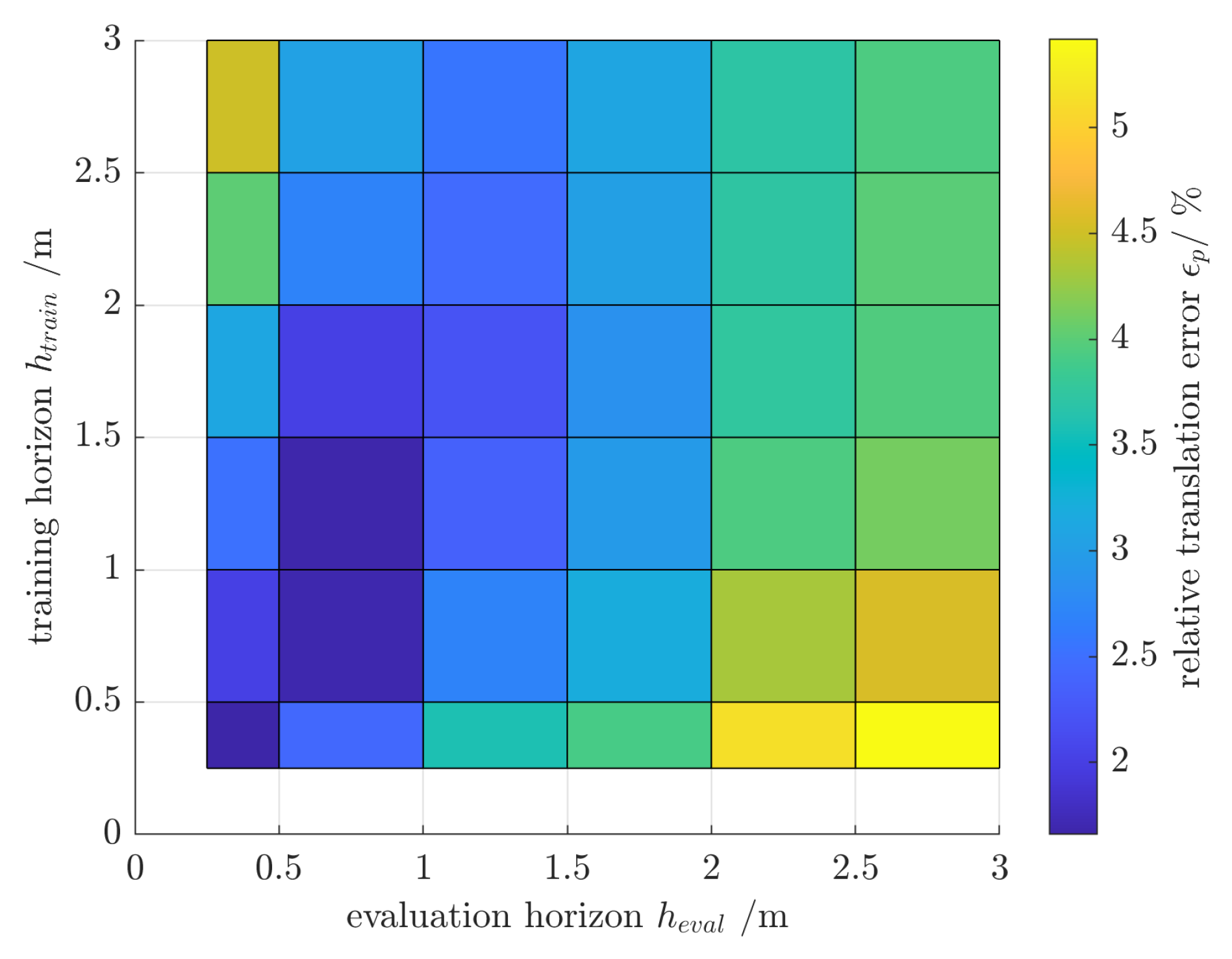
where is the ground truth and is the predicted state based on the linearized slip-aware motion model in discrete times. Minimizing J results in the optimal parameter vector . The trained model is evaluated over different data sets with the evaluation horizon . In this context, the evaluation horizon represents the prediction horizon for specific applications. The evaluation horizon is the indication of the prediction horizon of the model in the application. Assessing variable evaluation horizons with respect to variable training horizons is reveals the impact of different prediction horizons in the application compared to the parameter identification process.
To analyse the impact of different training and evaluation horizons, the mean relative translation/rotation errors are provided in Figure 9 and Figure 10. The analysis reveals that the best performance is achieved if the evaluation horizon is equal to (or less than) m. The error increases for larger deviation but remains bounded and lower than 5%.
3.2. Pose Prediction
The prediction model in (7), with elements from (4)–(6), is linearized around the operating point at each time step k in discrete times, where is the robot’s pose by the ego motion thread. The linear affine prediction model can be written as:
whereas the zero-mean term is due to model uncertainties. The discrete-time realization is approximated by
and
whereas are the continuous-time system and input matrices of the linearized prediction model, and for is the continuous-time state transition matrix expressed by the Peano-Baker series; the realization is assumed to not vary a lot in each interval , which is valid for the proposed cooperative mobile robot localization model with the sampling time ms. As a result, the bound of uncertainty due to the sampling time for discretization (in the slip-aware motion model) at the maximum speed of 1 m/s, at which the robot may experience wheel longitudinal slip, is 25 mm. Then, the expected state prediction from the ego motion thread is
whereas and ; the joint covariance for is then given by
The predicted covariance is
in which
Then, by using , the predicted covariance from the slip-aware motion model yields:
3.3. Augmented Localization
The visual thread and the ego motion thread communicate within the ROS framework through WiFi for the specific mobile robot test platform. To ensure proper data synchronization, time stamps are used to associate the visual-based localization (i.e., state estimation of ) to the corresponding pose estimation by the slip-aware model description. Delay in the communication, which is less than 20 ms for the tests conducted within 10 m of the stationary visual node (i.e., infrastructure-mounted stereo camera with the fisheye lens), is ignored in this section for the CI fusion. This is a valid assumption considering the sampling time ms for the pose prediction in the slip-aware motion model, the fusion part’s sampling time (i.e., 50 ms), and the maximum robot speed of 1 m/s at which the robot may experience wheel’s longitudinal slip. Denoting the estimation error in the slip-aware motion model at time step k by , and the visual thread by , we utilize the covariance intersection method having the upper bound of the mean square estimation error and the consistency condition.
Remark 2.
The asymptotic stable state transition matrix of the error dynamics in the motion model (9), and the geometrical filters for the visual-based depth estimation guarantee that the mean square estimation error (MSE) for the pose prediction model and the visual localization are upper bounded, i.e., and . As a result, the error covariance and of the estimated states from the two threads are consistent.
The estimated states from the ego motion thread and the visual thread are then fused using CI which is a convex combination of the covariances of the estimated states and guarantees a consistent error covariance (i.e., ). The CI is a geometric interpretation of
in which for all choices of , the covariance ellipses of the bound at level c,
lies within the intersection of covarinace ellipses of and , i.e., .
The weights will be obtained by minimizing a performance index on the bound , e.g., or , and consequently the covariance . The CI update strategy finds which encloses the intersection area and is consistent, although no knowledge about is available. The upper bounds of the covariance matrix elements for visual pose estimates is set to constant values derived from the error analysis (discussed in the next section) For the case where , the covariance can be given by
in which the optimal that minimize is obtained from the following constrained optimization program
where is the identity matrix with the proper dimension. The trace minimization program in (20) yields . As a result, the fusion of the estimated states from the ego motion and the visual threads is
where adjusts the assigned weights to and minimizing the performance index of the updated covariance.
According to the consistency in Remark 2 and the property of CI, it holds that
The heading of the robot is fused once the robot is close to the camera, thus, measurements are more accurate and reliable. The slip-aware observer and fusion is described in Algorithm 1.
| Algorithm 1: Augmented Slip-Aware Localization |
 |
4. Experiments and Discussion
The proposed infrastructure-aided localization framework is experimentally evaluated in this section through tests with harsh turning, cornering with acceleration/deceleration, and accelerated straight maneuvers which all include longitudinal slip at each wheel. The reference measurement and system setup is first discussed, then the experimental evaluations are provided. The wheel slip during harsh cornering, with nonholonomic constraints, results is reduced pose estimation accuracy for the existing odometry-based motion models which rely on wheel rotational speed. This has been addressed in this paper by the proposed slip-aware motion model (considering instantaneous centers of rotation) and the a multi-modal data fusion with the visual thread (even with distortion challenges imposed by low-cost fisheye lens).
The ground truth trajectory is recorded with the optical motion capture system Vicon Vantage V5. The test setup is composed of the Vicon system, the autonomous mobile robot (Jackal AGV), and the stationary stereo camera T265. The T265 is fixed mounted on a tripod at a height of 2 m and capturing the whole area where the tests are conducted. The robot is operating under the normal path-tracking mode and starting in front of the tripod of T265, with the speed between and 1 m/s, and mild and harsh cornering in tight and wide trajectories. In the proposed motion model, the wheel slip is indirectly quantified as a kinematic model parameter.
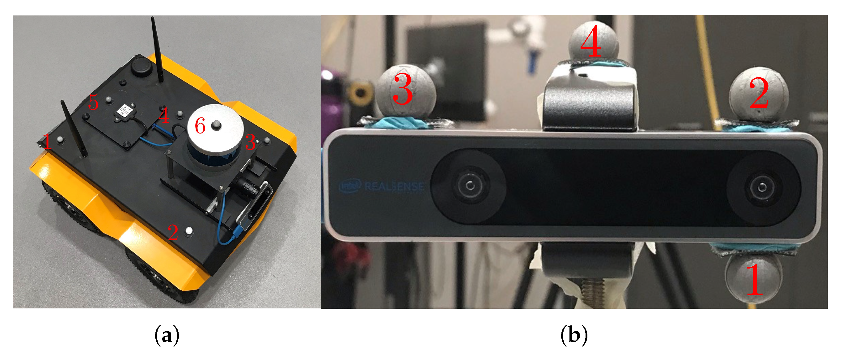
To detect the robot and initial setup of the stereo camera in the environment, passive markers are mounted on top of the robot and the stationary stereo camera, as shown in Figure 11, having sufficient distance for a rotation invariant geometry which is essential to ensure a unique pose and proper localization results using the Vicon system.
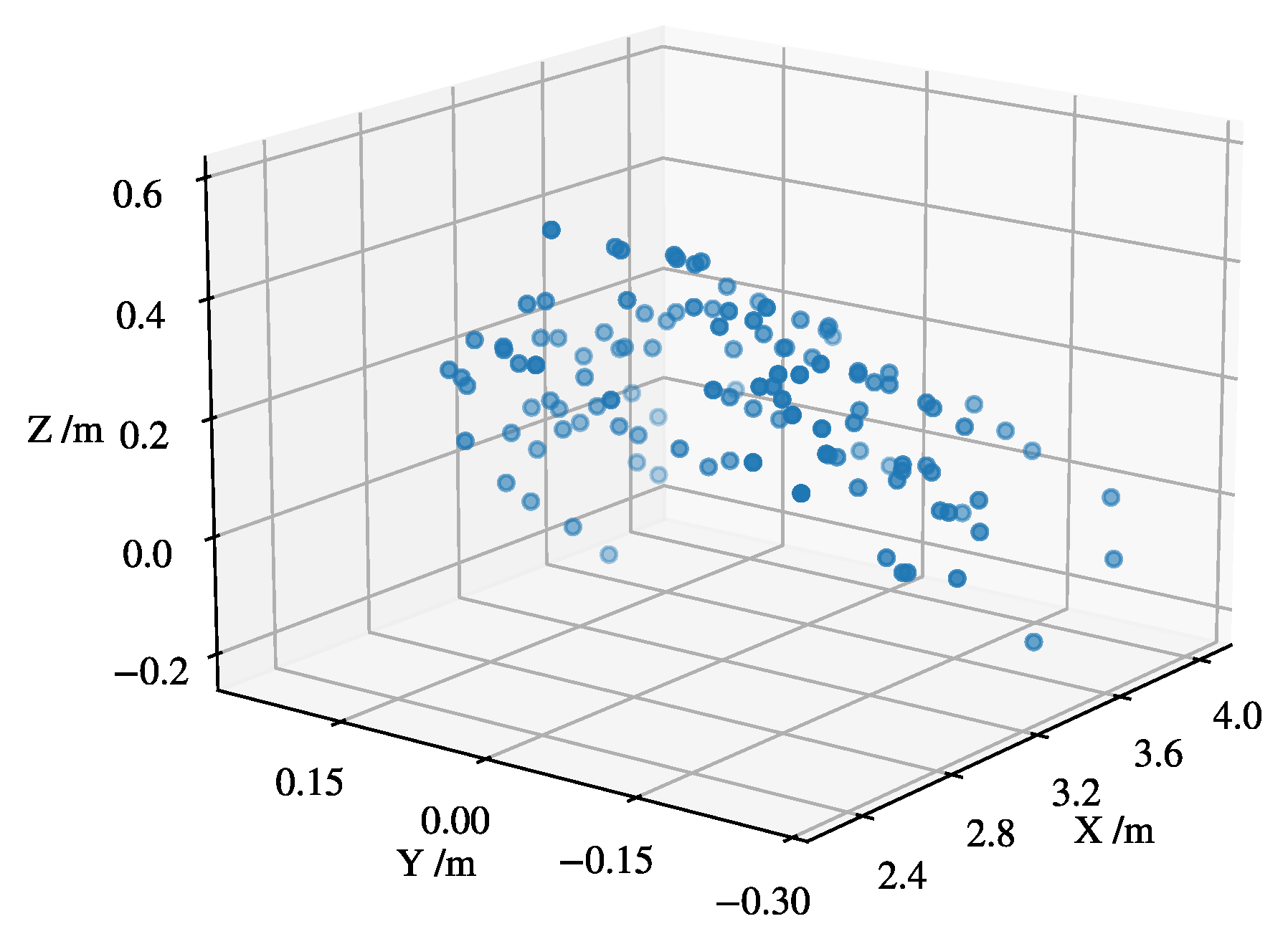
Figure 12 shows the visual point cloud of the robot detected under occlusion (by a human/user) in a long distance.
The ROI-based point cloud processing, which generates point cloud within the 2D bounding box of the detected robot, reduced computation time up to as has experimentally been tested with the robot in dynamic indoor environments with human presence. The processing time for the pose prediction based on the slip-aware motion model is almost <5 ms. There is no exhaustive recursive algorithm associate with the motion model part. The visual thread with the ROI-based processing takes up to 16 ms in various harsh turn and random cornering maneuvers. The fusion part with the trace optimization program on the visual and motion threads take up to 35 ms on the utilized embedded system in dynamic environments with human presence.
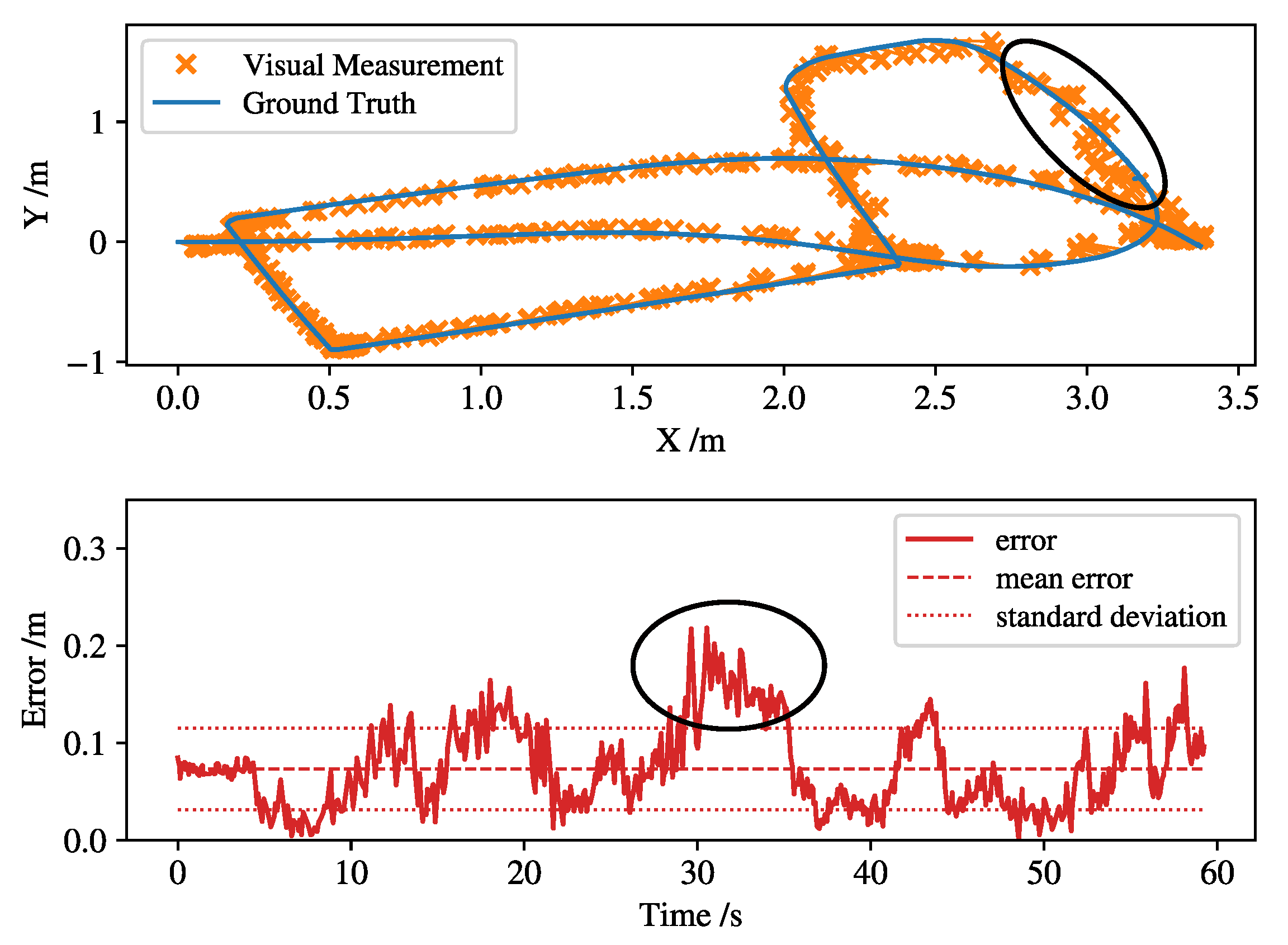
The position estimation error by the stereo visual thread is shown in Figure 13 for a maneuver with several tight cornering. The largest error of 21 cm is for the situation in which the robot is occluded (by a human/user in a shared working indoor environment) in a far (i.e., m) distance. The slip-aware motion model helps CI to recover the robot pose guaranteeing consistency of the estimation error covariance, i.e., .
The heading fusion result is depicted in Figure 14, where the heading prediction by the ego motion thread (without visual thread updates) is shown in dotted lines; this heading has large estimation error due to the harsh cornering scenarios and inaccuracies in the position of instantaneous center for the slip-aware ego motion model. The prediction fused with pose update from the visual thread in Figure 14 confirms better performance even with occlusion in this perceptually degraded test. This is due to the fact that the heading estimator (by the visual thread) employs multiple geometrical and nonholonomic constraints for the robot motion.
The position fusion results are illustrated in Figure 15 which confirms improvements in the estimation error when CI is applied using the visual thread to address uncertainties in the slip-aware ego motion thread in such arduous scenarios. The position prediction is fused with visual thread data, intentionally at each 200 ms to evaluate the effectiveness in large sample time updates or possible packet drop. Once the heading estimates are corrected by CI, the localization data is accurate with the root mean square error (RMSE) ≤ for several tests even with intermittent CI updates. The triangular shapes show the effect of the fusion process in which the kinematic motion model has been corrected and fused with the visual thread data. The kinematic model, a dead reckoning system, suffers from fault propagation and has an higher uncertainty as well as biased position prediction. Once the position is corrected with the visual localization, the corrected position and new initial position for the dead reckoning system moves close to the ground truth. Increasing the frequency of the update by the CI fusion will smooth the final estimates.
5. Conclusions
An augmented state estimation framework was proposed for localization of autonomous mobile robots in dynamic environments using infrastructure-mounted visual sensors and on-board data. The proposed system is composed of a visual tracking thread based on a stationary low-cost fisheye stereo camera mounted in the environment and a slip-aware ego motion thread that uses proprioceptive sensory data from a skid-steer mobile robot to enhance accuracy and reduce variance of the estimated states. The position and heading of the robot was estimated using the visual thread with a region of interest-based 3D point cloud processing which reduced the computation up to in dynamic indoor environments with human presence. This significantly enhances the real-time processing capability of the infrastructure-mounted sensing unit for localization and tracking of multi robots in indoor settings. A slip-aware kinematic model was developed for the ego motion thread to predict the robot pose, then, covariance intersection with guaranteed consistency was used to update the pose prediction with visual estimates, addressing slippage and occlusion for wheel odometry based state estimators and visual based localization in dynamic environments. The experimental results confirmed RMSE ≤17% and an average position accuracy of 7 cm for various tests even with intermittent (e.g., s) CI updates. The real time capability of the state estimation framework was confirmed by the computation time 35 ms for ROI-based visual processing and the fusion (through trace minimization). The future avenues include: (i) Using a motion model in the visual thread to enhance the consistency of the pose estimation; (ii) Integrating the IMU data into the ego motion thread and developing a motion model connecting wheel speeds, longitudinal slips, and robot dynamics within an optimization problem constrained to the robot kinematic/dynamic constrains to enhance orientation estimation.
Author Contributions
Conceptualization, E.H. and D.F.; methodology, D.F. and E.H.; writing, D.F. and N.P.B. and E.H.; simulation, D.F. and N.P.B.; data analysis, D.F. and E.H.; visualization, D.F.; review and editing, D.F. and E.H. and N.P.B.; funding acquisition E.H.; project administration E.H.; supervision, E.H. and D.F.; D.F. is with the Institute for Regulation and Control Systems, Karlsruhe Institute of Technology (KIT), Germany, and conducted his Master’s thesis at the NODE lab in Canada (under supervision of E.H.). All authors have read and agreed to the published version of the manuscript.
Funding
This work is supported by the Natural Science and Engineering Research Council of Canada, Discovery Grants RGPIN-05097-2020.
Institutional Review Board Statement
Not applicable.
Informed Consent Statement
Not applicable.
Data Availability Statement
Not applicable.
Acknowledgments
The authors thank University of Waterloo’s RoboHub for their valuable technical support, and Christian Bürkert Foundation for their financial support.
Conflicts of Interest
The authors declare no conflict of interest.
References
- Sun, D.; Geißer, F.; Nebel, B. Towards effective localization in dynamic environments. In Proceedings of the 2016 IEEE/RSJ International Conference on Intelligent Robots and Systems (IROS), Daejeon, Korea, 9–14 October 2016; pp. 4517–4523. [Google Scholar] [CrossRef]
- Campos, C.; Elvira, R.; Rodríguez, J.J.G.; Montiel, J.M.; Tardós, J.D. Orb-slam3: An accurate open-source library for visual, visual–inertial, and multimap slam. IEEE Trans. Robot. 2021, 37, 1874–1890. [Google Scholar] [CrossRef]
- Hess, W.; Kohler, D.; Rapp, H.; Andor, D. Real-time loop closure in 2D LIDAR SLAM. In Proceedings of the 2016 IEEE International Conference on Robotics and Automation (ICRA), Stockholm, Sweden, 16–21 May 2016; pp. 1271–1278. [Google Scholar]
- Shan, T.; Englot, B. Lego-loam: Lightweight and ground-optimized lidar odometry and mapping on variable terrain. In Proceedings of the 2018 IEEE/RSJ International Conference on Intelligent Robots and Systems (IROS), Madrid, Spain, 1–5 October 2018; pp. 4758–4765. [Google Scholar]
- Yang, P.; Freeman, R.A.; Lynch, K.M. Multi-agent coordination by decentralized estimation and control. IEEE Trans. Autom. Control 2008, 53, 2480–2496. [Google Scholar] [CrossRef]
- He, X.; Hashemi, E.; Johansson, K.H. Event-Triggered Task-Switching Control Based on Distributed Estimation. IFAC-PapersOnLine 2020, 53, 3198–3203. [Google Scholar] [CrossRef]
- Chung, H.Y.; Hou, C.C.; Chen, Y.S. Indoor intelligent mobile robot localization using fuzzy compensation and Kalman filter to fuse the data of gyroscope and magnetometer. IEEE Trans. Ind. Electron. 2015, 62, 6436–6447. [Google Scholar] [CrossRef]
- Qin, T.; Li, P.; Shen, S. Vins-mono: A robust and versatile monocular visual-inertial state estimator. IEEE Trans. Robot. 2018, 34, 1004–1020. [Google Scholar] [CrossRef]
- Berntorp, K. Joint wheel-slip and vehicle-motion estimation based on inertial, GPS, and wheel-speed sensors. IEEE Trans. Control Syst. Technol. 2016, 24, 1020–1027. [Google Scholar] [CrossRef]
- Zhou, S.; Liu, Z.; Suo, C.; Wang, H.; Zhao, H.; Liu, Y.H. Vision-based dynamic control of car-like mobile robots. In Proceedings of the 2019 International Conference on Robotics and Automation (ICRA), Montreal, QC, Canada, 20–24 May 2019; pp. 6631–6636. [Google Scholar]
- Chae, H.W.; Choi, J.H.; Song, J.B. Robust and Autonomous Stereo Visual-Inertial Navigation for Non-Holonomic Mobile Robots. IEEE Trans. Veh. Technol. 2020, 69, 9613–9623. [Google Scholar] [CrossRef]
- Tian, Y.; Sarkar, N. Control of a mobile robot subject to wheel slip. J. Intell. Robot. Syst. 2014, 74, 915–929. [Google Scholar] [CrossRef]
- Kubelka, V.; Oswald, L.; Pomerleau, F.; Colas, F.; Svoboda, T.; Reinstein, M. Robust data fusion of multimodal sensory information for mobile robots. J. Field Robot. 2015, 32, 447–473. [Google Scholar] [CrossRef]
- Delibasis, K.K.; Plagianakos, V.P.; Maglogiannis, I. Real time indoor robot localization using a stationary fisheye camera. In Proceedings of the IFIP International Conference on Artificial Intelligence Applications and Innovations; Springer: Berlin/Heidelberg, Germany, 2013; pp. 245–254. [Google Scholar]
- Janković, N.V.; Ćirić, S.V.; Jovičić, N.S. System for indoor localization of mobile robots by using machine vision. In Proceedings of the 2015 23rd Telecommunications Forum Telfor (TELFOR), Belgrade, Serbia, 24–26 November 2015; pp. 619–622. [Google Scholar]
- Mamduhi, M.H.; Hashemi, E.; Baras, J.S.; Johansson, K.H. Event-triggered Add-on Safety for Connected and Automated Vehicles Using Road-side Network Infrastructure. IFAC-PapersOnLine 2020, 53, 15154–15160. [Google Scholar] [CrossRef]
- Zickler, S.; Laue, T.; Birbach, O.; Wongphati, M.; Veloso, M. SSL-vision: The shared vision system for the RoboCup Small Size League. In Robot Soccer World Cup; Springer: Berlin/Heidelberg, Germany, 2009; pp. 425–436. [Google Scholar]
- Shim, J.H.; Cho, Y.I. A mobile robot localization via indoor fixed remote surveillance cameras. Sensors 2016, 16, 195. [Google Scholar] [CrossRef]
- Ramer, C.; Sessner, J.; Scholz, M.; Zhang, X.; Franke, J. Fusing low-cost sensor data for localization and mapping of automated guided vehicle fleets in indoor applications. In Proceedings of the 2015 IEEE International Conference on Multisensor Fusion and Integration for Intelligent Systems (MFI), San Diego, CA, USA, 14–16 September 2015; pp. 65–70. [Google Scholar]
- Ordonez, C.; Gupta, N.; Reese, B.; Seegmiller, N.; Kelly, A.; Collins, E.G., Jr. Learning of skid-steered kinematic and dynamic models for motion planning. Robot. Auton. Syst. 2017, 95, 207–221. [Google Scholar] [CrossRef]
- Liu, F.; Li, X.; Yuan, S.; Lan, W. Slip-aware motion estimation for off-road mobile robots via multi-innovation unscented Kalman filter. IEEE Access 2020, 8, 43482–43496. [Google Scholar] [CrossRef]
- Gosala, N.; Bühler, A.; Prajapat, M.; Ehmke, C.; Gupta, M.; Sivanesan, R.; Gawel, A.; Pfeiffer, M.; Bürki, M.; Sa, I.; et al. Redundant perception and state estimation for reliable autonomous racing. In Proceedings of the 2019 International Conference on Robotics and Automation (ICRA), Montreal, QC, Canada, 20–24 May 2019; pp. 6561–6567. [Google Scholar]
- Wang, D.; Low, C.B. Modeling and analysis of skidding and slipping in wheeled mobile robots: Control design perspective. IEEE Trans. Robot. 2008, 24, 676–687. [Google Scholar] [CrossRef]
- Rabiee, S.; Biswas, J. A friction-based kinematic model for skid-steer wheeled mobile robots. In Proceedings of the 2019 International Conference on Robotics and Automation (ICRA), Montreal, QC, Canada, 20–24 May 2019; pp. 8563–8569. [Google Scholar]
- Huang, J.; Wen, C.; Wang, W.; Jiang, Z.P. Adaptive output feedback tracking control of a nonholonomic mobile robot. Automatica 2014, 50, 821–831. [Google Scholar] [CrossRef]
- Mandow, A.; Martinez, J.L.; Morales, J.; Blanco, J.L.; Garcia-Cerezo, A.; Gonzalez, J. Experimental kinematics for wheeled skid-steer mobile robots. In Proceedings of the 2007 IEEE/RSJ International Conference on Intelligent Robots and Systems, San Diego, CA, USA, 29 October–2 November 2007; pp. 1222–1227. [Google Scholar]
- Marín, L.; Vallés, M.; Soriano, Á.; Valera, Á.; Albertos, P. Multi sensor fusion framework for indoor-outdoor localization of limited resource mobile robots. Sensors 2013, 13, 14133–14160. [Google Scholar] [CrossRef]
- Szeliski, R. Computer Vision: Algorithms and Applications; Springer Science & Business Media: Berlin/Heidelberg, Germany, 2010. [Google Scholar]
- Kannala, J.; Brandt, S.S. A generic camera model and calibration method for conventional, wide-angle, and fish-eye lenses. IEEE Trans. Pattern Anal. Mach. Intell. 2006, 28, 1335–1340. [Google Scholar] [CrossRef]
- Bochkovskiy, A.; Wang, C.Y.; Liao, H.Y.M. YOLOv4: Optimal Speed and Accuracy of Object Detection. arXiv 2020, arXiv:2004.10934. [Google Scholar]
- Rublee, E.; Rabaud, V.; Konolige, K.; Bradski, G. ORB: An efficient alternative to SIFT or SURF. In Proceedings of the 2011 International Conference on Computer Vision, Barcelona, Spain, 6–13 November 2011; pp. 2564–2571. [Google Scholar]
- Gupta, S.; Kumar, M.; Garg, A. Improved object recognition results using SIFT and ORB feature detector. Multimed. Tools Appl. 2019, 78, 34157–34171. [Google Scholar] [CrossRef]
- Holz, D.; Ichim, A.E.; Tombari, F.; Rusu, R.B.; Behnke, S. Registration with the point cloud library: A modular framework for aligning in 3-D. IEEE Robot. Autom. Mag. 2015, 22, 110–124. [Google Scholar] [CrossRef]
- Munaro, M.; Rusu, R.B.; Menegatti, E. 3D robot perception with point cloud library. Robot. Auton. Syst. 2016, 78, 97–99. [Google Scholar] [CrossRef]
Figure 1.
The slip-aware localization framework overview.

Figure 2.
The mobile robot platform and the coordinates.

Figure 3.
The visual tracking thread with ROI.

Figure 4.
Epipolar geometry for non-rectified stereo images.

Figure 5.
Unrectified stereo images with fisheye distortion.

Figure 6.
Rectified and undistorted stereo images.

Figure 7.
Robot point cloud post processed by the statistical outlier filter. The robot is in the closest position to the stereo camera. The outer dimension of the points is used for a Euclidean distance based sparsity as a measure to be close to the actual geometry of the Jackal robot.
Figure 7.
Robot point cloud post processed by the statistical outlier filter. The robot is in the closest position to the stereo camera. The outer dimension of the points is used for a Euclidean distance based sparsity as a measure to be close to the actual geometry of the Jackal robot.

Figure 8.
IC-based skid steer kinematics for the motion model.

Figure 9.
Relative translational error of the motion model parameter identification for varying training and evaluation horizons on the same ground classification (i.e., gravel or asphalt).
Figure 9.
Relative translational error of the motion model parameter identification for varying training and evaluation horizons on the same ground classification (i.e., gravel or asphalt).

Figure 10.
Relative angular error of the motion model parameter identification for varying training and evaluation horizons on the same ground classification (i.e., gravel or asphalt).
Figure 10.
Relative angular error of the motion model parameter identification for varying training and evaluation horizons on the same ground classification (i.e., gravel or asphalt).

Figure 11.
The experimental setup using Vicon (a) Clearpath’s Jackal robot equipped with 16-line LiDARs (from RoboSense or Velodyne) for motion planning and controls in dynamic environments (b) Infrastructure-mounted low-cost stereo vision for the augmented localization through dedicated short-range communication with the on-board state estimator.

Figure 12.
Robot point cloud with a statistical outlier filter for a detection with partial occlusion in a dynamic environment in a far (i.e., m) range. This depicts the effect of far detection and partial occlusion (by an object/human) on the quality and sparsity of the point cloud used for clustering and pose estimation; with a predicted longitudinal dimension of 2 m in x-direction, the point cloud does not corresponds the robot dimension. The CI based fusion resolves partial occlusion/detection as will be illustrated for pose estimation later in this section.

Figure 13.
Position estimation results based on Euclidean center of the point cloud from the mobile robot. The T265 camera is located at position (0,0) facing the longitudinal x-direction. The largest error occurs at the maximum relative position (indicated with a black ellipse) between the robot and infrastructure-mounted stereo camera.

Figure 14.
Orientation estimation by the infrastructure-aided localization framework.

Figure 15.
Position estimates by the infrastructure-aided localization; slip-aware motion model handles occlusion and uncertainties in the point cloud computation for the robot detection in far distances.
Figure 15.
Position estimates by the infrastructure-aided localization; slip-aware motion model handles occlusion and uncertainties in the point cloud computation for the robot detection in far distances.

Publisher’s Note: MDPI stays neutral with regard to jurisdictional claims in published maps and institutional affiliations. |
© 2022 by the authors. Licensee MDPI, Basel, Switzerland. This article is an open access article distributed under the terms and conditions of the Creative Commons Attribution (CC BY) license (https://creativecommons.org/licenses/by/4.0/).
Share and Cite
MDPI and ACS Style
Flögel, D.; Bhatt, N.P.; Hashemi, E. Infrastructure-Aided Localization and State Estimation for Autonomous Mobile Robots. Robotics 2022, 11, 82. https://doi.org/10.3390/robotics11040082
AMA Style
Flögel D, Bhatt NP, Hashemi E. Infrastructure-Aided Localization and State Estimation for Autonomous Mobile Robots. Robotics. 2022; 11(4):82. https://doi.org/10.3390/robotics11040082
Chicago/Turabian StyleFlögel, Daniel, Neel Pratik Bhatt, and Ehsan Hashemi. 2022. "Infrastructure-Aided Localization and State Estimation for Autonomous Mobile Robots" Robotics 11, no. 4: 82. https://doi.org/10.3390/robotics11040082
Note that from the first issue of 2016, this journal uses article numbers instead of page numbers. See further details here.