
Planar Model for Vibration Analysis of Cable Rehabilitation Robots


Department of Industrial Engineering, University of Padova, Via Venezia 1, 35131 Padova, Italy
*
Author to whom correspondence should be addressed.
Robotics 2022, 11(6), 154; https://doi.org/10.3390/robotics11060154
Submission received: 29 September 2022
/
Revised: 4 November 2022
/
Accepted: 16 December 2022
/
Published: 18 December 2022
(This article belongs to the Special Issue Advanced Technologies in Rehabilitation Robots: Design, Control, and Human–Robot Interaction)
Abstract
:Cable robots are widely used in the field of rehabilitation. These robots differ from other cable robots because the cables are rather short and are usually equipped with magnetic hooks to improve the ease of use. The vibrations of rehabilitation robots are dominated by the effects of the hooks and payloads, whereas the cables behave as massless springs. In this paper, a 2D model of the cables of a robot that simulates both longitudinal and transverse vibrations is developed and experimentally validated. Then the model is extended to simulate the vibrations of an actual 3D robot in the symmetry planes. Finally, the calculated modal properties (natural frequencies and modes of vibration) are compared with the typical spectrum of excitation due to the cable’s motion. Only the first transverse mode can be excited during the rehabilitation exercise.
1. Introduction
There are millions of individuals in the world who currently experience various movement-related disabilities [1] frequently as a result of sensory impairments, traumatic brain injuries (TBI), and musculoskeletal and neurological disorders [2,3]. Multiple review articles and meta-analyses have considered the benefits of rehabilitation and medical robotics [4,5,6,7,8,9,10] and many researchers have argued that robotic rehabilitation devices (RRDs) that emphasize intense [11], highly repetitive [12,13], and task-oriented [14] movements allows for assisting rehabilitation training and recovering the functions of patient’s limbs [15,16,17,18].
Typical power transmissions of RRDs include gear-driven, cable-driven, belt-driven, and ball-screw-driven transmissions [19]. Compared to the other types, cable-driven rehabilitation robots (CDRRs) offer several promising features such as low inertia, high payload-to-weight ratio, and large workspaces [20,21,22]. Moreover, CDRRs actuators are usually fixed to the ground, strongly reducing the mass to be moved; pulleys are used to allow changes in the orientation of the cables, while the payload is connected to the cables via hooks. Due to such features, many CDRRs have been proposed over the years [23,24,25,26,27,28,29], and many more are in development these days [30,31,32,33]. Although CDRRs have a lot of promising features, there are also some limitations and deficiencies due to the intrinsic properties of cables, which result in unidirectional power transmission, vibrations, and maintenance. These limitations increase the complexity of kinematic and dynamic modeling of CDRRs [34]. The elasticity or flexibility of cables of CDRRs causes undesirable vibrations, which may generate position and orientation errors and compromise patient comfort. The importance of magnetic hooks is mostly related to flexibility. In fact, the orthosis (i.e., the payload of the rehabilitation robot) can be detached and can be fitted to a patient while another one is performing an exercise. Moreover, thanks to the hooks, different orthoses can be installed, both passive [24] and active [35].
In a previous study [36], the effects of hook mass and pulley inertia on a cable-driven rehabilitation robot were analyzed. Each cable was schematized by a 4-DOF model (the so-called “simplified cable system”) and both the longitudinal and transverse vibrations were considered. The final results show that the first longitudinal natural frequency does not significantly depend on the mass of the hook and on the inertia of the pulley. In addition, the inertia of the pulley also does not affect the transverse natural frequencies. Therefore, in the extension of the single cable vibrational model to a planar model with two cables, it is possible to simplify the system by neglecting the effects of the inertia of pulleys and of the mass of the hook in the longitudinal direction.
To the best of the author’s knowledge, no previous work on CDRRs has discussed the modes of vibration of cable robots equipped with hooks. The motivation behind this paper is to propose a vibration analysis of a cable system that reproduces the characteristics of a wire-driven rehabilitation robot. Since massless cables are assumed, cable sagging is negligible. This assumption is acceptable for applications that do not involve large workspaces [37,38].
Starting from the cable system of the rehabilitation robot, in Section 2 a planar model that evaluates natural frequencies and modes of vibration is proposed, then the planar model is extended to a 3D analysis of modes of vibration. In both cases, the stable equilibrium configurations were first analyzed and free vibrations of these configurations were studied. The numerical results and the effect of the system’s parameters on the natural frequencies are reported in Section 3. The comparison between the analytical and the experimental data is made in Section 4. In Section 5, the relation between the frequency content of the input motion and the natural frequencies is discussed. Finally, future applications of the cable model are illustrated and conclusions are drawn.
2. Mathematical Model for the Free Vibrations
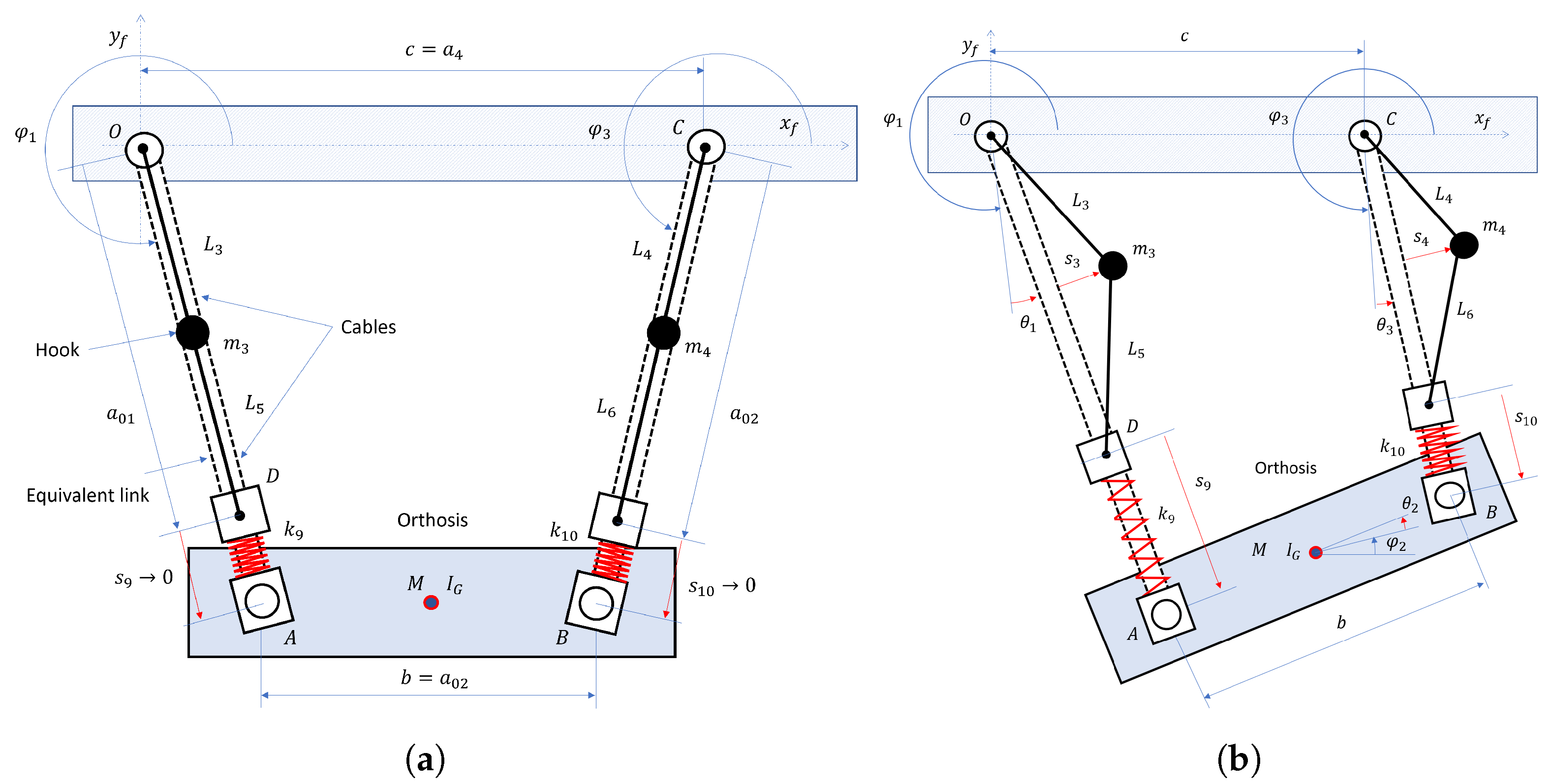
The Maribot [29,39] (Figure 1a) is a 5-DOF CDRR composed of a rigid planar structure (2-DOF) and a yielding structure moved by cables (3-DOF). The three cables are controlled by DC motors fixed to rigid links, and they support an orthosis used to hold up the patient’s arm during rehabilitation exercises (Figure 1b). Cable length and orientation are determined by the presence of pulleys. To improve the ease of use, each cable is connected to a magnetic hook near the orthosis, moreover, it allows the instantaneous release of the cable when a safety-limit force is overcome. Other examples of this kind of structure can be seen in some CDRRs such as in [23,24,25,26].
2.1. Planar Model
To extend the single cable vibrational model developed in [36] to a planar model with two cables, the system in Figure 2 was considered. The planar model is composed of two cables ( and ) which connect the pulleys (considered to be mechanically fixed since their inertia does not affect the transverse natural frequency) to the magnetic hooks (mass and ). Moreover, the negligible influence of the pulleys allows us to simplify the model of the horizontal cables and that connect the motors to the pulleys since they do not influence transverse vibrations, and their longitudinal stiffness combines in series with the stiffness of the other cables. A payload equivalent to 2/3 of the expected load on the orthosis (mass M) is supported by two cables with length and . To take into account cable elastic deformation, two linear springs connect the lower cables to the orthosis. This planar model is useful to simplify the analysis of the actual 3D model, which will be reported in Section 2.2.
To generalize the planar model, the 4-bar linkage was considered. It is composed of three mobile links with variable lengths and a fixed link with constant length (). In the initial configuration (Figure 2a) the cables overlap the equivalent links and . The deflections of the springs and , which account for cable longitudinal deformations, are zero (the deformations due to the static load are taken into account in the initial lengths of the cables). The main motion of the 4-bar linkage is described by rotations with respect to the fixed reference system. The vibration analysis of the system requires considering the small rotation of each link (), with respect to the configuration defined by and link elongation (Figure 2b). Therefore, the link length is:
where is the initial length of the link i and is the elongation of the link i.
The scalar equations of the vector loop of the 4-bar linkage are:
since .
When the analysis of small oscillations of the linkage is carried out, rotations are assumed constant and payload length is constant. The system has 3 DOFs, which can be associated with small rotation and to elongations and . Indeed, and are dependent on the other degrees of freedom via Equation (2).
The initial lengths of the links are equal to:
where b is the length of the payload and c is the distance between cable pulleys. Assuming small oscillations, the elongation of links 1 and 3 can be calculated as:
where the first terms and are the displacements due to longitudinal cable elongations, whereas the second terms are caused by the transverse displacements of the hooks ( and ), and can be derived by simple geometric considerations [36]. Actually, the transverse displacement of hook 1 causes a small displacement of point D along the ideal link () rotated by . The same happens on link 3 due to the transverse displacement of link 2.
Then, Equation (2) is expanded considering first-order approximations of the trigonometric functions of small angles , , and . The following equation holds, which makes it possible to calculate the dependent variables ( and ) as functions of the independent variables (, , and ), which are contained in vector .
where vector is equal to:
Solving and collecting, the small rotations and are equal to:
Equation (4) shows that and include both first-order terms and second-order terms. In the framework of small oscillations analysis, the second-order terms can be neglected in the calculation of kinetic energy. Therefore, the following simplified equations of link angular velocities hold:
A stable equilibrium configuration has to be found before performing a free vibration analysis. In [40], it was shown that, if the two cables have the same length and if the CoM of the payload lies halfway to the payload link, the configuration with , , is stable ( is an arbitrary constant value); therefore, small oscillations about this configuration are considered in this research. Strictly speaking, in [40] the mass of the hooks was not taken into account, but, if this mass is small and the system is symmetric, the cable system with hooks has the same stable configurations as the system without hooks.
The equations of motion are derived with Lagrange’s approach, the generalized coordinates are , , , , .
In the hypothesis of massless cables, kinetic energy and elastic and gravity potential energy ( and ) are:
where M and are the payload mass and inertia, respectively, and and are the stiffnesses of the linear springs that represent the stiffness of the left cables in series (, and ) and of the right cables (, and ). The first-order approximations used to calculate the velocities in (11) are:
The calculation of gravity potential energy requires second-order approximations of the vertical positions of masses in Equation (13). These expressions are obtained from the loop Equation (2) considering second-order approximations of the trigonometric functions and neglecting higher-order terms.
Using Lagrange’s approach, the equations of free undamped vibrations in matrix form are obtained:
where is the mass matrix, is the stiffness matrix of the system, and . The mass and stiffness matrices of the general planar model have the following structures:
where the first three rows (coordinates , , and ) represent the transverse vibrations of the cables, and the last two rows (coordinates and ) represent the longitudinal vibrations.
If the 4-bar linkage OABC is a parallelogram with links , , , and , the mass and stiffness matrices become:
In the parallelogram configuration, the structure of the mass and stiffness matrices clearly shows that the longitudinal vibrations of the cables are decoupled with transverse vibrations. Finally, natural frequencies and modes of vibration are calculated by solving the eigenvalue problem.
2.2. 3D Simplified Model
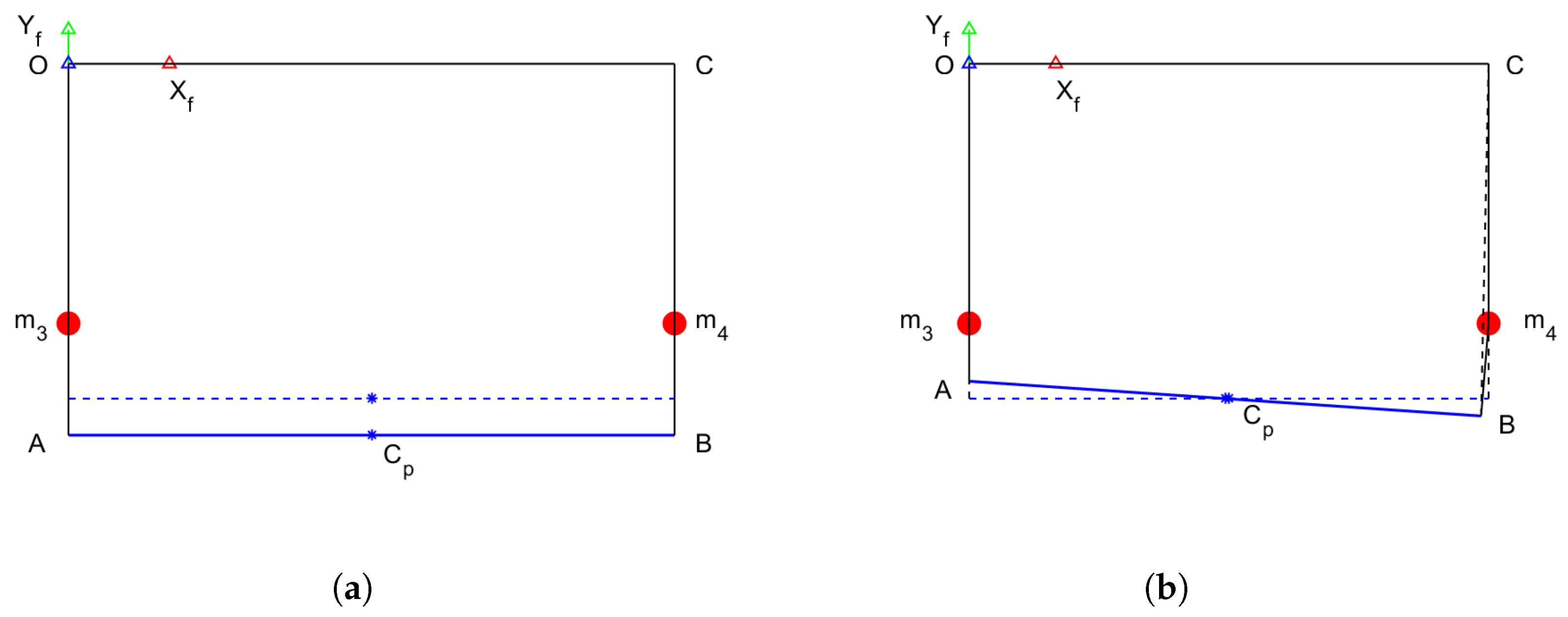
To extend the planar model to a simplified 3D model, an approach similar to the one proposed in [40] was used. The three upper extremities of the cables (, , and ) are assumed to lie on the same horizontal plane and form an equilateral triangle with side length . The attachment points of the magnetic hooks (, , and ) and of the payload (, , and ) form equilateral triangles as well, where the side length of the payload triangle is equal to . The center of mass of the payload coincides with the centroid of triangle . Moreover, the three upper cables have the same length as well as the three lower cables . The initial configuration is shown in Figure 3, in which there are three vertical planes of symmetry.
If the object swings in one of these three vertical planes, e.g., (P and Q are the middle points of and , respectively), it is equivalent to the motion of a planar cable system in the same vertical plane. Hence, the motion of such a 3D cable system in its vertical planes of symmetry can be regarded as the motion of an equivalent planar 4-bar linkage.
As reported in [40], in this case, the 4-bar linkage is not symmetric ( and the CoM is not halfway the payload link); nevertheless, the configuration of Figure 3 is still stable. In conclusion, the modes of vibration of the 3D system can be simply calculated considering the modes of vibration of each equivalent vertical plane.
3. Numerical Results
The link dimensions of the model are based on the actual lengths of the cable robot. In turn, the dimensions of the cable robot depend on the patient’s size and on the rehabilitation exercise. To perform calculations, typical values are chosen and reported in Table 1.
The natural frequencies are calculated by solving the eigenvalue problem associated with Equation (18). To facilitate the analysis of modes of vibration, it is possible to exploit the decoupling of the system, analyzing the vibration modes for submatrixes. In particular, modes I, II, and III, related to the transverse displacements are analyzed separately from modes IV and V, which are related to the longitudinal displacements. The transverse and longitudinal natural frequencies are shown in Table 2.
To evaluate the influence of the stiffness of the horizontal cables, the natural frequencies of the modes of vibration are calculated considering or neglecting the lengths of cables and . The comparison reported in Table 2 shows that all the transverse modes are not affected by the horizontal cables, while in the longitudinal modes the effect of the horizontal cables leads to a deviation of about 12%. Since the transverse frequencies and modes are the most involved during the rehabilitation exercises (as will be demonstrated in Section 5), the influence of horizontal cables will be neglected and the following results will consider only the effect of vertical cables , and , .
In Figure 4, the decoupling between the longitudinal and transverse modes is numerically investigated also for the general planar model. Indeed, considering and , for the natural frequencies of the modes vary less than 1.5% with respect to the values calculated with . Therefore, the terms , , , in and in in Equation (19) are negligible, and the transverse vibrations can be considered numerically decoupled from the longitudinal vibrations.
3.1. Transverse Modes of Vibration
In Figure 5, the transverse modes of vibration of the planar system are represented. In mode I, rotation is dominant, consequently, the system behaves like a parallelogram with the orthosis translating on the plane (anti-symmetric configuration). Mode II is dominated by the transverse translations of the magnetic hooks ( and ) in the counter-phase, maintaining a symmetrical configuration. Mode III is anti-symmetric like mode I, but the translation of the hooks is larger than the rotation of the system.
3.2. Longitudinal Modes of Vibration
In Figure 6, the longitudinal modes of vibrations of the planar system are represented. In this case, mode IV corresponds to a translation of the orthosis (bounce motion), while mode V corresponds to a rotation of the orthosis in the plane due to and displacements in the counter-phase (pitch motion).
3.3. Modes of Vibration of the 3D System
To analyze the modes of vibration of the 3D system, the stable and admissible equilibrium configuration of a three cables system proposed in [40] was considered. In order to calculate the modes of vibration of the orthosis in the vertical plane passing through the patient’s forearm, the generalized planar model of Figure 2b is applied in the vertical plane . The sides and are equal to the heights of the equilateral triangles and and are horizontal. The sides and are, instead, inclined by and deriving from the study of the equilibrium configuration of the quadrilateral as explained in [40]. The mass is equal to the mass of the rear hook , while the mass is equal to the sum of the masses of the front hooks and .
3.4. Influence of Parameters on Natural Frequencies
Maribot is a neurorehabilitation robot developed to rehabilitate acute and subacute patients after a stroke. For this reason, the robot configurations have to adapt to the clinical conditions of each patient (e.g., sitting or lying in bed). Therefore, the length of the cables changes not only during each exercise but also based on the clinical conditions. It is worth noticing that the variation in cable length leads to a variation in cable stiffness according to the following equation:
where , , and and , , and are the Young modulus and the section area of cables, respectively, and , , and are the lengths of the cables.
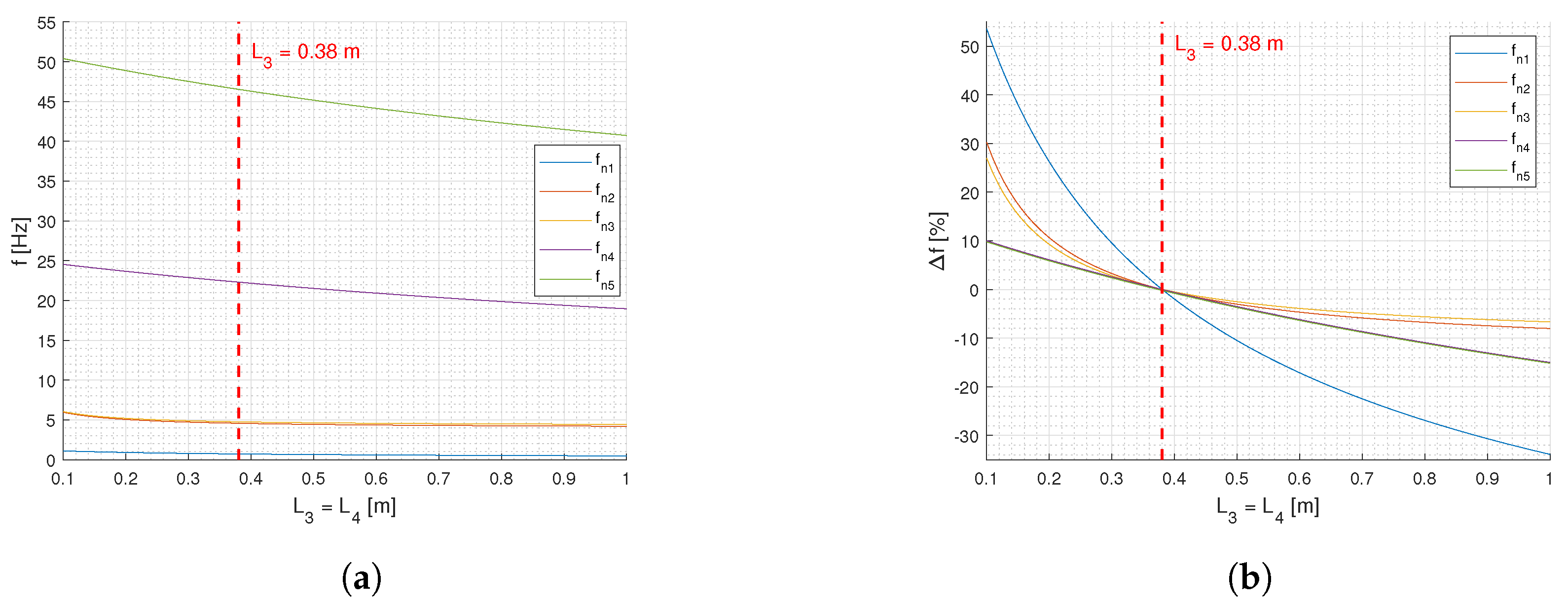
Since the variation in cable length leads to a variation in the natural frequency of the structure, it is useful to study the correlation between the cable length and the natural frequency. The parallelogram configuration was considered. In Figure 8a, cables 3 and 4 vary their lengths between 0.1 and 1.0 m and such an increase in length leads to a reduction in the resonance frequency for each mode.
In Figure 8b, the natural frequency of each mode is normalized with respect to the maximum value of each resonance frequency. In this case, the largest percentage of variation is obtained with the transverse modes, with a variation that varies from to in the first mode.
A global analysis of the influence of the parameters presented in Table 1, which refers to parallelogram configuration, can be performed using radar plots. Figure 9 shows the variation in the natural frequency of each mode of vibration that corresponds to a set of multiple values of each parameter (nominal value , , , , and ).
It is worth noticing that the variation in the length of the cables and of 3 and 5 times is easily achievable during rehabilitation exercises. Conversely, the lengths of the cables and , the masses, and the distance between cables vary by a little amount by changing patient or exercise. The lengths of cable and are fixed and are not considered in the radar plots.
Starting from the value of the nominal parameters reported in Table 1, by increasing the length of cables and , all the natural frequencies decrease. In particular, considering the distance between curves, the length of cables 3 and 4 has a larger influence on the natural frequency of mode I, while the length of cables 5 and 6 has a larger effect on the resonance frequency in the other modes. Conversely, the increase in the payload mass M leads to an increase in the resonance frequencies of modes II and III, and to a decrease in the frequency of modes IV and V. The variation in payload mass has no significant effect on the natural frequency of mode I. If the mass of the magnetic hook increases, the natural frequencies of modes II and III decrease. The mass of the hook has a very small effect on mode I and no effect on modes IV and V. The distance between the cables has no influence on the natural frequency of all modes.
4. Experimental Test and Validation
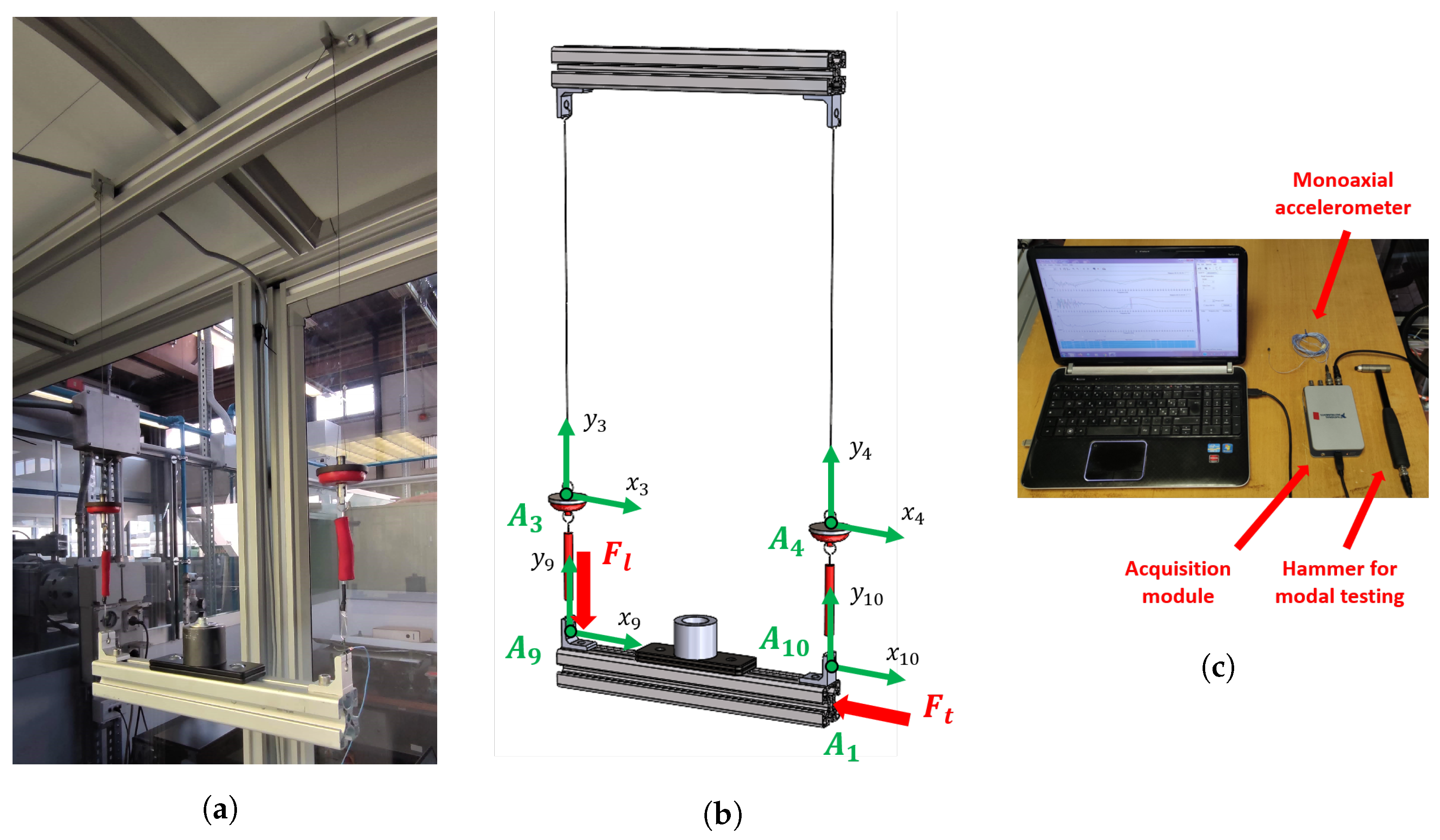
To experimentally validate the planar model of Section 2, an orthosis with an arm was simulated by means of a mock-up composed of an aluminum profile mm with a mass of 406 g and an additional mass of 706 g above the center of gravity of the bar (total mass: g). According to the results reported in Table 2, the stiffness of horizontal cables and do not influence transverse vibrations. Therefore, the magnetic hooks are directly connected to the chassis via Dyneema cables with lengths and and spaced apart by 300 mm. At the extremity of the aluminum profile, the lower ends of the nylon cables are hooked, while at the opposite ends they are connected to the magnetic hooks. A representation of the experimental planar cable system is shown in Figure 10a.
The tests were carried out with the modal analysis approach [41], which is widely used in fields of automotive engineering [42,43], aerospace engineering [44], automatic machines [45], and robotics [46].
Two kinds of experimental tests were performed: the first with transverse excitation and acceleration, and the second with longitudinal excitation and acceleration. In each test configuration, the excitation was always exerted at a fixed point in the defined direction (transverse for modes I, II, and III, and longitudinal for modes IV and V), whereas acceleration was measured in the various grid points reported in Figure 10b. The excitation was performed by means of a PCB 086C03 hammer (with load cell sensitivity 2.25 mV/N), while the acceleration was measured by a PCB 352C23 monoaxial accelerometer (sensitivity mV/g) built by PCB Piezotronics Inc., Depew, NY, USA (Figure 10c). In the transverse tests the axis of the accelerometer was always perpendicular to the cable in the plane of motion, whereas, in the longitudinal tests the axis of the accelerometer was always aligned to the cables. Data were acquired using a NI9234 data acquisition board built by National Instruments, Austin, TX, USA with a sampling frequency of 2048 Hz, and samples for transverse modes of vibration and 4096 samples for longitudinal modes. This sampling frequency allows us to analyze the vibration phenomena up to 1024 Hz, and, as shown by the calculated analytical results, the natural frequencies of the modes of vibration are well below this frequency. Measured signals were analyzed by means of ModalVIEW, a specific software tool for modal analysis. In this way, for both configurations, four FRFs were measured between the acceleration components and the hammer impact force. To improve the reliability and quality of measurements, each FRF was calculated by averaging the results obtained with three hammer blows. Measured data were then processed with ModalVIEW to identify the natural frequencies, modal dampings, and modal shapes.
Analytical and experimental results are compared in Table 4. Considering the nominal lengths mm, both in transverse and longitudinal directions, the experimental results confirm the results of the simplified analytical model with a deviation smaller than 13%.
The FRFs measured with transverse excitation are reported in Figure 11a. The first index of the FRF represents the position and direction of measured acceleration, whereas the second index represents the position and direction of the hammer blow. The first mode of vibration, experimentally detected at Hz shows amplitudes of the FRFs of nodes 9 and 10 (on the mock-up) larger than the ones of nodes 3 and 4 of the magnetic hooks, which is consistent with Figure 5a.
The second and third modes of vibration were detected at and Hz (due to excitation ). At this frequency, the amplitudes of nodes 3 and 4 are larger than the ones of nodes 9 and 10, again in agreement with modes II and III, as reported in Figure 5a,b.
Coming to the results obtained with longitudinal excitation, Figure 11b shows that vibration modes IV and V, experimentally detected, respectively, at and Hz, have larger oscillation amplitudes for nodes 9 and 10 than for nodes 3 and 4.
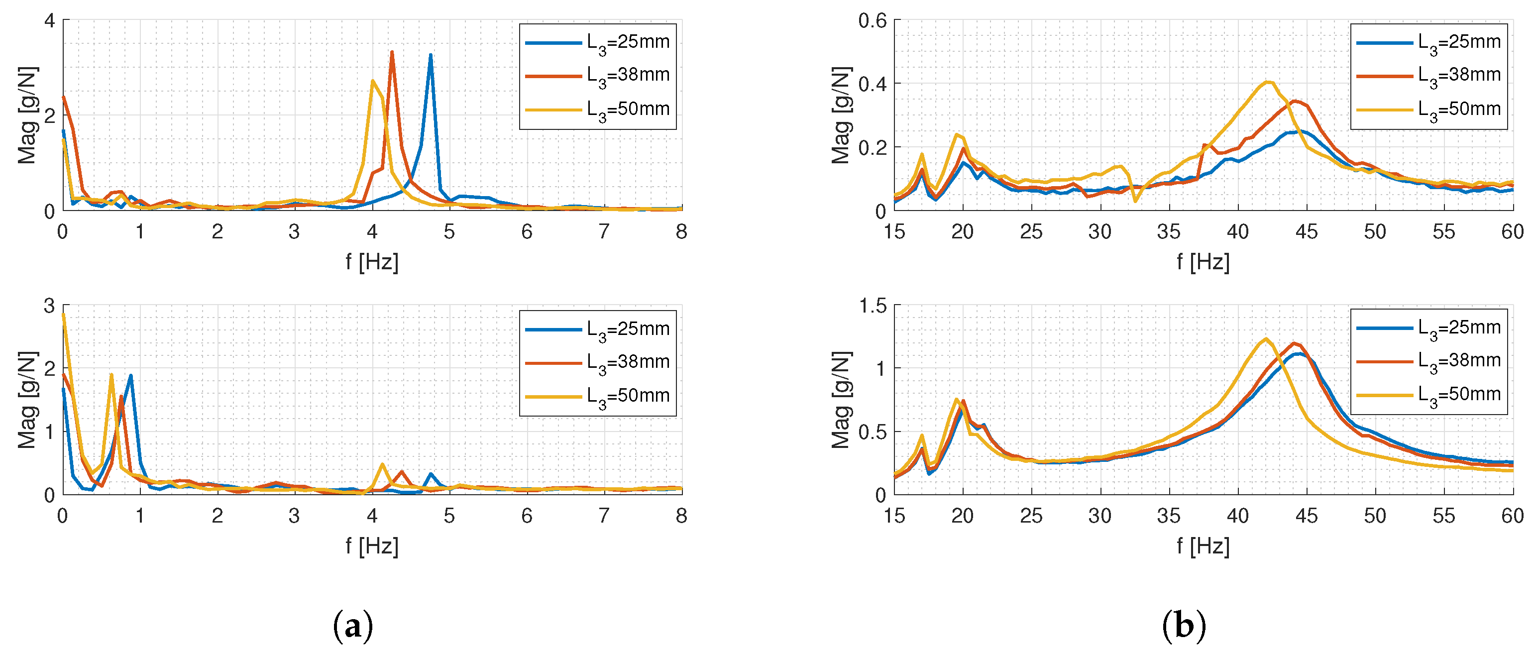
Further experimental tests were carried out to validate the effect of the variations in cable lengths predicted by the numerical model. Results are reported in Figure 12 that show the moduli of the FRFs of nodes 2 and 4 in the presence of transverse (Figure 12a) and longitudinal (Figure 12b) excitation. The peaks of the FRFs, which are related to the modes of vibration, move as cable lengths change; nevertheless, the variation is rather small (e.g., the natural frequency of the first transverse mode is always in the range of 0.6–1 Hz). Table 4 makes a comparison between the measured and calculated natural frequencies. In both new cases ( mm and mm), the experimental measurements confirm the results of the calculated natural frequencies with a deviation smaller than 16%.
5. Frequency Content of the Input Motion
Rehabilitation exercises are performed cyclically by varying both the vertical and horizontal positions of the orthosis. The vertical motion is obtained by changing the length of the cables, whereas the horizontal motion is performed by the joints of the planar robot. Both motions can excite the vibrations of the suspended system (cables + orthosis). The frequency spectrum of excitation has to be compared with the natural frequencies of the modes of vibration to evaluate the possible excitation of the suspended system in resonance conditions. The typical cycle of a rehabilitation exercise has a duration of 20 s, which corresponds to a fundamental frequency of Hz, which is well below the natural frequencies of the transverse and longitudinal modes of vibration of the suspended system. Nevertheless, the motion has not a simple harmonic law and higher-order harmonics may be present. The vertical motion is performed by varying the lengths of all the cables with the same motion law. In this example, a 5-degree polynomial law [47] was adopted to vary the cable lengths from the minimum to the maximum value.
In Figure 13, the time histories and the fast Fourier transforms (FFT) of the acceleration and velocity of the cables are reported.
Considering the FFT of the acceleration, Figure 13a shows that the longitudinal natural frequencies of the cable system are not excited by the periodic input motion, since the FFT tends to zero above Hz. The transverse modes of the system are poorly excited by the longitudinal accelerations of cables, but it can be noticed that the acceleration spectrum has a small amplitude at the frequency of the first transverse mode, which is represented by the vertical bar with the label . Conversely, the transverse modes are excited by the Coriolis force, which depends on the velocity of the cables and the velocity of oscillation of the structure. Therefore, the frequency content of the velocity profile was investigated as reported in Figure 13b. In this case, the first natural frequency is not excited during the motion, since the FFT tends to zero over Hz.
The horizontal motion is performed by actuating the joints of the planar robot and it can excite the transverse vibrations of the suspended system. Additionally, in this case, the frequency spectrum of the acceleration of the upper extremities of the cables was calculated and the results showed that higher-order harmonics are not able to excite the transverse modes.
6. Conclusive Remarks
A mathematical model taking into account the special features of a CDRR equipped with magnetic hooks was developed. The results show that in most practical cases transverse vibrations are decoupled from longitudinal vibrations due to cable longitudinal compliance. Both in longitudinal and transverse directions, the natural frequencies and modes of vibration were numerically calculated and validated through experimental tests, which demonstrated the reliability of the analytical model with a deviation smaller than . Then, considering the vertical planes of symmetry of the actual 3D model, the planar model was extended to a 3D analysis of modes of vibration of the Maribot cable system.
The motion of the cables (variation in length) during the exercises has two effects: the variation in the natural frequencies of the system and the excitation of the system. A parametric analysis showed that the variation in the lengths of the cables during the exercise has the largest effect on the natural frequency of the first transverse mode; nevertheless, this frequency is always in the range of 0.5–1.0 Hz.
The analysis of the typical motion laws used in rehabilitation exercises showed that the suspended system is not excited in resonance if the cycle of the rehabilitation exercise has a duration of about 20 s.
A future development will be the improvement of the 3D model of the orthosis to take into account details of the stiffness and mass proprieties. Moreover, the joint reaction forces on the magnetic hooks will be studied and the model will be extended to study forced vibrations.
Author Contributions
Conceptualization, G.Z., A.D., M.B., and G.R.; methodology, A.D. and G.R.; software, G.Z. and M.B.; validation, G.Z. and M.B.; formal analysis, A.D. and M.B.; investigation, G.Z., A.D., M.B., and G.R.; writing—original draft preparation, G.Z., A.D., and M.B.; writing—review and editing, A.D. and G.R.; visualization, G.Z. and A.D.; supervision, A.D. and G.R.; project administration, A.D. All authors have read and agreed to the published version of the manuscript.
Funding
This research received no external funding.
Data Availability Statement
Not applicable.
Conflicts of Interest
The authors declare no conflict of interest.
References
- Babaiasl, M.; Mahdioun, S.H.; Jaryani, P.; Yazdani, M. A review of technological and clinical aspects of robot-aided rehabilitation of upper-extremity after stroke. Disabil. Rehabil. Assist. Technol. 2016, 11, 263–280. [Google Scholar] [CrossRef] [PubMed]
- Maciejasz, P.; Eschweiler, J.; Gerlach-Hahn, K.; Jansen-Troy, A.; Leonhardt, S. A survey on robotic devices for upper limb rehabilitation. J. Neuroeng. Rehabil. 2014, 11, 1–29. [Google Scholar] [CrossRef] [PubMed] [Green Version]
- Cieza, A.; Causey, K.; Kamenov, K.; Hanson, S.W.; Chatterji, S.; Vos, T. Global estimates of the need for rehabilitation based on the Global Burden of Disease study 2019: A systematic analysis for the Global Burden of Disease Study 2019. Lancet 2020, 396, 2006–2017. [Google Scholar] [CrossRef] [PubMed]
- Hobbs, B.; Artemiadis, P. A review of robot-assisted lower-limb stroke therapy: Unexplored paths and future directions in gait rehabilitation. Front. Neurorobot. 2020, 14, 19. [Google Scholar] [CrossRef] [Green Version]
- Weber, L.M.; Stein, J. The use of robots in stroke rehabilitation: A narrative review. NeuroRehabilitation 2018, 43, 99–110. [Google Scholar] [CrossRef] [Green Version]
- Bertani, R.; Melegari, C.; De Cola, M.C.; Bramanti, A.; Bramanti, P.; Calabrò, R.S. Effects of robot-assisted upper limb rehabilitation in stroke patients: A systematic review with meta-analysis. Neurol. Sci. 2017, 38, 1561–1569. [Google Scholar] [CrossRef]
- Chien, W.T.; Chong, Y.Y.; Tse, M.K.; Chien, C.W.; Cheng, H.Y. Robot-assisted therapy for upper-limb rehabilitation in subacute stroke patients: A systematic review and meta-analysis. Brain Behav. 2020, 10, e01742. [Google Scholar] [CrossRef] [PubMed]
- Narayan, J.; Kalita, B.; Dwivedy, S.K. Development of robot-based upper limb devices for rehabilitation purposes: A systematic review. Augment. Hum. Res. 2021, 6, 1–33. [Google Scholar] [CrossRef]
- Zuccon, G.; Lenzo, B.; Bottin, M.; Rosati, G. Rehabilitation robotics after stroke: A bibliometric literature review. Expert Rev. Med Devices 2022, 19, 405–421. [Google Scholar] [CrossRef]
- Moshaii, A.A.; Najafi, F. A review of robotic mechanisms for ultrasound examinations. Ind. Robot. Int. J. 2014, 41, 373–380. [Google Scholar] [CrossRef]
- Nelles, G. Cortical reorganization-effects of intensive therapy. Restor. Neurol. Neurosci. 2004, 22, 239–244. [Google Scholar] [PubMed]
- Bütefisch, C.; Hummelsheim, H.; Denzler, P.; Mauritz, K.H. Repetitive training of isolated movements improves the outcome of motor rehabilitation of the centrally paretic hand. J. Neurol. Sci. 1995, 130, 59–68. [Google Scholar] [CrossRef] [PubMed]
- French, B.; Thomas, L.H.; Coupe, J.; McMahon, N.E.; Connell, L.; Harrison, J.; Sutton, C.J.; Tishkovskaya, S.; Watkins, C.L. Repetitive task training for improving functional ability after stroke. Cochrane Database Syst. Rev. 2016, 11, CD006073. [Google Scholar] [CrossRef] [Green Version]
- Bayona, N.A.; Bitensky, J.; Salter, K.; Teasell, R. The role of task-specific training in rehabilitation therapies. Top. Stroke Rehabil. 2005, 12, 58–65. [Google Scholar] [CrossRef] [PubMed]
- Cao, J.; Xie, S.Q.; Das, R.; Zhu, G.L. Control strategies for effective robot assisted gait rehabilitation: The state of art and future prospects. Med. Eng. Phys. 2014, 36, 1555–1566. [Google Scholar] [CrossRef]
- Oujamaa, L.; Relave, I.; Froger, J.; Mottet, D.; Pelissier, J.Y. Rehabilitation of arm function after stroke. Literature review. Ann. Phys. Rehabil. Med. 2009, 52, 269–293. [Google Scholar] [CrossRef]
- Ceccarelli, M.; Bottin, M.; Russo, M.; Rosati, G.; Laribi, M.; Petuya, V. Requirements and Solutions for Motion Limb Assistance of COVID-19 Patients. Robotics 2022, 11, 45. [Google Scholar] [CrossRef]
- Prasad, R.; El-Rich, M.; Awad, M.; Hussain, I.; Jelinek, H.; Huzaifa, U.; Khalaf, K. A Framework for Determining the Performance and Requirements of Cable-Driven Mobile Lower Limb Rehabilitation Exoskeletons. Front. Bioeng. Biotechnol. 2022, 10, 920462. [Google Scholar] [CrossRef]
- Gopura, R.; Bandara, D.; Kiguchi, K.; Mann, G.K. Developments in hardware systems of active upper-limb exoskeleton robots: A review. Robot. Auton. Syst. 2016, 75, 203–220. [Google Scholar] [CrossRef]
- Bruckmann, T.; Pott, A. Cable-Driven Parallel Robots; Springer: Berlin/Heidelberg, Germany, 2012; Volume 12. [Google Scholar]
- Khosravi, M.A.; Taghirad, H.D. Dynamic modeling and control of parallel robots with elastic cables: Singular perturbation approach. IEEE Trans. Robot. 2014, 30, 694–704. [Google Scholar] [CrossRef]
- Kawamura, S.; Kino, H.; Won, C. High-speed manipulation by using parallel wire-driven robots. Robotica 2000, 18, 13–21. [Google Scholar] [CrossRef]
- Mao, Y.; Jin, X.; Dutta, G.G.; Scholz, J.P.; Agrawal, S.K. Human movement training with a cable driven arm exoskeleton (CAREX). IEEE Trans. Neural Syst. Rehabil. Eng. 2014, 23, 84–92. [Google Scholar] [CrossRef] [PubMed]
- Rosati, G.; Gallina, P.; Masiero, S. Design, implementation and clinical tests of a wire-based robot for neurorehabilitation. IEEE Trans. Neural Syst. Rehabil. Eng. 2007, 15, 560–569. [Google Scholar] [CrossRef] [PubMed]
- Ball, S.J.; Brown, I.E.; Scott, S.H. A planar 3DOF robotic exoskeleton for rehabilitation and assessment. In Proceedings of the 2007 29th Annual International Conference of the IEEE Engineering in Medicine and Biology Society, Lyon, France, 22–26 August 2007; IEEE: Piscataway, NJ, USA, 2007; pp. 4024–4027. [Google Scholar]
- Perry, J.C.; Rosen, J.; Burns, S. Upper-limb powered exoskeleton design. IEEE/ASME Trans. Mechatron. 2007, 12, 408–417. [Google Scholar] [CrossRef]
- Laribi, M.; Ceccarelli, M.; Sandoval, J.; Bottin, M.; Rosati, G. Experimental Validation of Light Cable-Driven Elbow-Assisting Device L-CADEL Design. J. Bionic Eng. 2022, 19, 416–428. [Google Scholar] [CrossRef]
- Zuccon, G.; Bottin, M.; Ceccarelli, M.; Rosati, G. Design and performance of an elbow assisting mechanism. Machines 2020, 8, 68. [Google Scholar] [CrossRef]
- Rosati, G.; Gallina, P.; Masiero, S.; Rossi, A. Design of a new 5 dof wire-based robot for rehabilitation. In Proceedings of the 9th International Conference on Rehabilitation Robotics, ICORR 2005, Chicago, IL, USA, 28 June–1 July 2005; IEEE: Piscataway, NJ, USA, 2005; pp. 430–433. [Google Scholar]
- Xu, P.; Li, J.; Li, S.; Xia, D.; Zeng, Z.; Yang, N.; Xie, L. Design and Evaluation of a Parallel Cable-Driven Shoulder Mechanism With Series Springs. J. Mech. Robot. 2022, 14, 031012. [Google Scholar] [CrossRef]
- Xu, Z.; Xie, L. Cable-Driven Flexible Exoskeleton Robot for Abnormal Gait Rehabilitation. J. Shanghai Jiaotong Univ. Sci. 2022, 27, 231–239. [Google Scholar] [CrossRef]
- Seyfi, N.; Keymasi Khalaji, A. Robust control of a cable-driven rehabilitation robot for lower and upper limbs. ISA Trans. 2022, 125, 268–289. [Google Scholar] [CrossRef]
- Zhong, B.; Guo, K.; Yu, H.; Zhang, M. Toward Gait Symmetry Enhancement via a Cable-Driven Exoskeleton Powered by Series Elastic Actuators. IEEE Robot. Autom. Lett. 2022, 7, 786–793. [Google Scholar] [CrossRef]
- Shoaib, M.; Asadi, E.; Cheong, J.; Bab-Hadiashar, A. Cable driven rehabilitation robots: Comparison of applications and control strategies. IEEE Access 2021, 9, 110396–110420. [Google Scholar] [CrossRef]
- Rosati, G.; Cenci, S.; Boschetti, G.; Zanotto, D.; Masiero, S. Design of a single-dof active hand orthosis for neurorehabilitation. In Proceedings of the 2009 IEEE International Conference on Rehabilitation Robotics, Kyoto, Japan, 23–26 June 2009; pp. 161–166. [Google Scholar]
- Zuccon, G.; Tang, L.; Doria, A.; Bottin, M.; Minto, R.; Rosati, G. The Effect of Pulleys and Hooks on the Vibrations of Cable Rehabilitation Robots. In Mechanisms and Machine Science, Proceedings of the Advances in Italian Mechanism Science, Naples, Italy, 7–9 September 2022; Springer: Berlin/Heidelberg, Germany, 2022; Volume 122, pp. 273–281. [Google Scholar]
- Kozak, K.; Zhou, Q.; Wang, J. Static analysis of cable-driven manipulators with non-negligible cable mass. IEEE Trans. Robot. 2006, 22, 425–433. [Google Scholar] [CrossRef]
- Riehl, N.; Gouttefarde, M.; Krut, S.; Baradat, C.; Pierrot, F. Effects of non-negligible cable mass on the static behavior of large workspace cable-driven parallel mechanisms. In Proceedings of the 2009 IEEE International Conference on Robotics and Automation, Kobe, Japan, 12–17 May 2009; IEEE: Piscataway, NJ, USA, 2009; pp. 2193–2198. [Google Scholar]
- Rosati, G.; Andreolli, M.; Biondi, A.; Gallina, P. Performance of cable suspended robots for upper limb rehabilitation. In Proceedings of the 2007 IEEE 10th International Conference on Rehabilitation Robotics, Noordwijk, The Netherlands, 13–15 June 2007; IEEE: Piscataway, NJ, USA, 2007; pp. 385–392. [Google Scholar]
- Jiang, Q.; Kumar, V. Determination and stability analysis of equilibrium configurations of objects suspended from multiple aerial robots. J. Mech. Robot. 2012, 4, 021005. [Google Scholar] [CrossRef]
- Ewins, D.J. Modal Testing: Theory, Practice and Application; John Wiley & Sons: Hoboken, NJ, USA, 2009. [Google Scholar]
- Cossalter, V.; Doria, A.; Mitolo, L. Inertial and modal properties of racing motorcycles. SAE Trans. 2002, 111, 2461–2468. [Google Scholar]
- Cossalter, V.; Doria, A.; Basso, R.; Fabris, D. Experimental analysis of out-of-plane structural vibrations of two-wheeled vehicles. Shock Vib. 2004, 11, 433–443. [Google Scholar] [CrossRef] [Green Version]
- Verbeke, J.; Debruyne, S. Vibration analysis of a UAV multirotor frame. In Proceedings of the ISMA 2016 International Conference on Noise and Vibration Engineering, Leuven, Belgium, 19–21 September 2016; pp. 2401–2409. [Google Scholar]
- Belotti, R.; Caneva, G.; Palomba, I.; Richiedei, D.; Trevisani, A. Model updating in flexible-link multibody systems. J. Phys. Conf. Ser. 2016, 744, 012073. [Google Scholar] [CrossRef] [Green Version]
- Doria, A.; Cocuzza, S.; Comand, N.; Bottin, M.; Rossi, A. Analysis of the compliance properties of an industrial robot with the Mozzi axis approach. Robotics 2019, 8, 80. [Google Scholar] [CrossRef]
- Biagiotti, L.; Melchiorri, C. Trajectory Planning for Automatic Machines and Robots; Springer: Berlin/Heidelberg, Germany, 2008. [Google Scholar]
Figure 1.
Maribot: (a) rehabilitation robot; (b) orthosis and cable system.

Figure 2.
Scheme of the analytical planar model: (a) initial configuration of the 4-bar linkage; (b) model with elongations and rotations of links.
Figure 2.
Scheme of the analytical planar model: (a) initial configuration of the 4-bar linkage; (b) model with elongations and rotations of links.

Figure 3.
The 3D analytical model.

Figure 4.
Correlation between natural frequencies and : (a) trend of natural frequencies; (b) trend of natural frequencies normalized by the nominal natural frequency of each mode ().
Figure 4.
Correlation between natural frequencies and : (a) trend of natural frequencies; (b) trend of natural frequencies normalized by the nominal natural frequency of each mode ().

Figure 5.
Transverse modes of vibration: (a) mode I; (b) mode II; (c) mode III.

Figure 6.
Longitudinal modes of vibration: (a) mode IV; (b) mode V.

Figure 7.
Modes of vibration of the 3D system: (a) mode I; (b) mode II; (c) mode III; (d) mode IV; (e) mode V.
Figure 7.
Modes of vibration of the 3D system: (a) mode I; (b) mode II; (c) mode III; (d) mode IV; (e) mode V.


Figure 8.
Correlation between natural frequency and cable length : (a) trend of frequency; (b) trend of frequency normalized by the nominal natural frequency of each mode (m).
Figure 8.
Correlation between natural frequency and cable length : (a) trend of frequency; (b) trend of frequency normalized by the nominal natural frequency of each mode (m).

Figure 9.
Influence of parameters on the natural frequency for each mode of vibration. The value of parameters reported in Table 1 are multiplied by . (a) mode I; (b) mode II; (c) mode III; (d) mode IV; (e) mode V.
Figure 9.
Influence of parameters on the natural frequency for each mode of vibration. The value of parameters reported in Table 1 are multiplied by . (a) mode I; (b) mode II; (c) mode III; (d) mode IV; (e) mode V.

Figure 10.
(a) Experimental cable system; (b) measurement points and directions of measurement of the accelerometer (green); excitation forces (red); (c) acquisition equipment.
Figure 10.
(a) Experimental cable system; (b) measurement points and directions of measurement of the accelerometer (green); excitation forces (red); (c) acquisition equipment.

Figure 11.
Modulus (above) and phase (below) of the experimental FRFs: (a) transverse modes; (b) longitudinal modes. The first index represents the measurement point and direction, whereas the second index represents the excitation point and direction.
Figure 11.
Modulus (above) and phase (below) of the experimental FRFs: (a) transverse modes; (b) longitudinal modes. The first index represents the measurement point and direction, whereas the second index represents the excitation point and direction.

Figure 12.
Experimental FRFs modulus in nodes 2 (above) and 4 (below); (a) transverse excitation; (b) longitudinal excitation.
Figure 12.
Experimental FRFs modulus in nodes 2 (above) and 4 (below); (a) transverse excitation; (b) longitudinal excitation.

Figure 13.
Periodic input motion of a five-degree polynomial in the time domain (upper) and frequency domain (lower): (a) acceleration profile; (b) velocity profile.
Figure 13.
Periodic input motion of a five-degree polynomial in the time domain (upper) and frequency domain (lower): (a) acceleration profile; (b) velocity profile.


Table 1.
Parameters of the mathematical model.
| Parameter | Value |
|---|---|
| (kg · m) | |
| M (kg) | |
| (kg) | |
| g (m/s) | |
| (m) | |
| (m) | |
| (m) | |
| (m) | |
| (rad) | |
| (rad) | 0 |
Table 2.
Influence of horizontal cables and in the analytical natural frequencies.
| Transverse (Hz) | Mode I | 0.720 | 0.720 | 0 |
| Mode II | 4.571 | 4.571 | 0 | |
| Mode III | 4.756 | 4.756 | 0 | |
| Longitudinal (Hz) | Mode IV | 19.868 | 22.305 | 12.27 |
| Mode V | 41.622 | 46.725 | 12.26 |
Table 3.
Natural frequencies of the analytical 3D model.
| Mode I | Mode II | Mode III | Mode IV | Mode V | |
|---|---|---|---|---|---|
| f (Hz) | 0.731 | 3.846 | 4.078 | 18.414 | 35.753 |
Table 4.
Comparison between analytical and experimental natural frequencies with different cable lengths.
Table 4.
Comparison between analytical and experimental natural frequencies with different cable lengths.
| (mm) | Mode | Analytical (Hz) | Experimental (Hz) | Experimental | ||
|---|---|---|---|---|---|---|
| 0.25 | Transverse | I | 0.842 | 0.834 | 0.455 | 0.95% |
| II | 4.858 | 4.407 | 0.656 | 9.28% | ||
| III | 5.028 | 4.735 | 0.574 | 5.83% | ||
| Longitudinal | IV | 23.261 | 19.878 | 5.868 | 14.54% | |
| V | 48.729 | 44.578 | 5.938 | 8.52% | ||
| 0.38 | Transverse | I | 0.720 | 0.715 | 1.491 | 0.69% |
| II | 4.571 | 3.977 | 0.530 | 12.99% | ||
| III | 4.756 | 4.280 | 0.637 | 10.01% | ||
| Longitudinal | IV | 22.305 | 19.688 | 4.818 | 11.73% | |
| V | 46.725 | 44.121 | 5.268 | 5.57% | ||
| 0.50 | Transverse | I | 0.644 | 0.634 | 0.816 | 1.55% |
| II | 4.432 | 3.725 | 0.548 | 15.95% | ||
| III | 4.646 | 4.056 | 0.701 | 12.70% | ||
| Longitudinal | IV | 21.520 | 19.218 | 3.178 | 10.70% | |
| V | 45.079 | 42.126 | 4.675 | 6.55% | ||
Publisher’s Note: MDPI stays neutral with regard to jurisdictional claims in published maps and institutional affiliations. |
© 2022 by the authors. Licensee MDPI, Basel, Switzerland. This article is an open access article distributed under the terms and conditions of the Creative Commons Attribution (CC BY) license (https://creativecommons.org/licenses/by/4.0/).
Share and Cite
MDPI and ACS Style
Zuccon, G.; Doria, A.; Bottin, M.; Rosati, G. Planar Model for Vibration Analysis of Cable Rehabilitation Robots. Robotics 2022, 11, 154. https://doi.org/10.3390/robotics11060154
AMA Style
Zuccon G, Doria A, Bottin M, Rosati G. Planar Model for Vibration Analysis of Cable Rehabilitation Robots. Robotics. 2022; 11(6):154. https://doi.org/10.3390/robotics11060154
Chicago/Turabian StyleZuccon, Giacomo, Alberto Doria, Matteo Bottin, and Giulio Rosati. 2022. "Planar Model for Vibration Analysis of Cable Rehabilitation Robots" Robotics 11, no. 6: 154. https://doi.org/10.3390/robotics11060154
Note that from the first issue of 2016, this journal uses article numbers instead of page numbers. See further details here.